Effective universality in quantum gravity

Asymptotically safe matter-gravity systems and their physics can be described in terms of the effective action $\Gamma[\bar{g}_{\mu\nu},h_{\mu\nu},\varphi]$ in a gauge-fixed setting. In the effective action we have dropped the Faddeev-Popov ghosts and restricted ourselves to the case with scalar matter described by $\varphi$. The field $h_{\mu\nu}$ denotes dynamical metric fluctuations around a generic background metric $\bar{g}_{\mu\nu}$. The occurrence of the latter comes hand in hand with the gauge fixing. The relation between background metric and fluctuation field is not necessarily linear, but in the present work we consider the linear split

$\displaystyle g_{\mu\nu}=\bar{g}_{\mu\nu}+\sqrt{Z_{h}G_{N}}\,h_{\mu\nu}\,,$

(1)

with the graviton wave-function renormalisation $Z_{h}$ normalised to one at some RG scale $\Lambda$. In (1) we have dropped the wave-function renormalisations of $g_{\mu\nu},\bar{g}_{\mu\nu}$ for the sake of readability. The $G_{N}$-factor leads to a fluctuation field $h_{\mu\nu}$ with the canonical dimension one. The effective action $\Gamma[\bar{g}_{\mu\nu},h_{\mu\nu},\varphi]$ is not diffeomorphism-invariant, but satisfies non-trivial Slavnov-Taylor identities (STIs). The information on physics is carried by the diffeomorphism-invariant effective action,

$\displaystyle\Gamma[g_{\mu\nu},\varphi]=\Gamma[g_{\mu\nu},h_{\mu\nu}=0,\varphi]\,.$

(2)

and the respective background correlation functions are related to S-matrix elements. However, their computations requires the knowledge of the scattering processes with dynamical gravitons $h_{\mu\nu}$. These processes are described through different couplings $G_{\vec{n}}$, where the vector $\vec{n}$ consists of the numbers of the different dynamical fields $\Phi=\big(h_{\mu\nu},\,c_{\mu},\,\varphi,\,\dots\big)$ that take part in the process,

$\displaystyle\vec{n}=\big(n_{h},\,n_{c},\,n_{\varphi},\,\dots\big)\,.$

(3)

The couplings $G_{\vec{n}}$ of all these fields to the dynamical graviton are avatars of the gravitational self-coupling $G_{N}$. In the present study we concentrate on gravity-scalar couplings. This leaves us with couplings labelled by two indices only,

$\displaystyle G_{(n_{h},n_{\varphi})}\,.$

(4)

We denote dimensionless versions of the Newton coupling by capital letters, e.g. as above $G_{(n_{h},n_{\varphi})}$, and dimensionful versions with an additional over-bar, such as $\bar{G}_{(n_{h},n_{\varphi})}$. The fluctuation couplings $G_{(n_{h},n_{\varphi})}$ defined in (4) are related to the expansion coefficients in an expansion in powers of $h_{\mu\nu}$, the couplings $G_{(n_{\bar{g}},n_{\varphi})}$ are related to those in an expansion in powers of $\bar{g}_{\mu\nu}$. The respective vertices are given by

		$\displaystyle\Gamma^{(n,m,l)}(p_{1},\ldots,p_{n+m+l})$
		$\displaystyle\qquad=\frac{\delta^{n+m+l}\Gamma[\bar{g},h,\varphi]}{\delta\bar{g}^{n}(p_{1},\ldots)\delta h^{m}(\ldots,p_{i},\ldots)\delta\varphi^{l}(\ldots,p_{n+m+l})}\,,$		(5)

where we suppress the indices on $\bar{g}$ and $h$ for brevity of notation. The couplings (4) are now defined by (5) at selected kinematic configurations. In this work, we focus on $G_{(3,0)}$ and $G_{(1,2)}$ defined at the momentum-symmetric point. The former coupling relates to the scattering of three gravitons, and is derived from the pure gravity part of the effective action. The coupling $G_{(1,2)}$ relates to the scattering of one graviton and two scalars, and is derived from the kinetic term of the scalars. This coupling is also present in the free -no self-interaction- scalar theory and can be considered the fundamental coupling of scalar fields to gravity. We compare these couplings based on their flow equations. We do not compute the explicit STIs that relate them. In general the information from the flow and the STIs is equivalent, but in a truncated non-perturbative computation they will not agree. It is an important task to quantify to what extent the STIs are satisfied but this goes beyond the scope of this work. The computation of the STIs is a technically challenging task, for an example in QCD see [87, 88].

Evidently these couplings cannot be defined uniquely and depend on the given kinematical limit. Note that this even holds for dimensionless couplings beyond one loop, despite their universal RG running. Accordingly, the evaluation of, e.g., scattering processes with different momentum configurations requires an analysis of the corresponding $n$-point vertex as a function of all its independent momenta, i.e., a simple function of one momentum cannot capture the full dynamics adequately. If dealing with an approximation to the theory that does not maintain the full momentum-dependence of vertices, a typical choice is the symmetric point, for higher-order vertices a symmetric point. Using these momentum configurations can lead to semi-quantitative agreement with the full results even in strongly-correlated systems, for recent work in gravity see [6], and in QCD see [88]. For a related discussion in the effective field theory approach to gravity see [89]. Keeping this caveat in mind, we proceed with our study whether avatars of the Newton coupling, defined using the symmetric momentum configuration of various three-point vertices, show semi-quantitative agreement.

With the dynamical vertices (5) and the dynamical propagators we can compute the background vertices, that is the $S$-matrix elements. This leads to further avatars of the Newton coupling, this time being directly related to S-matrix elements for the selected momentum configuration. In the present work we consider the avatar of the Newton coupling of the background curvature term in the action. It is distinguished from the $G_{\vec{n}}$ by two properties: first it is the prefactor of a diffeomorphism invariant term in the action. Second, as a pure background quantity it does not drive the RG flow of the system, which is driven by the fluctuation field and its couplings. In this work, we refer to its dimensionless version as $\bar{G}$ and the dimensionful version as $G_{N}$.

The standard approach to computations in asymptotically safe gravity is the functional renormalisation group (FRG). The FRG approach to quantum gravity is based on the flow equation for the effective action, the Wetterich equation [90, 91, 92],

	$\displaystyle\partial_{t}\Gamma_{k}=\frac{1}{2}{\rm Tr}\left[G_{k}\,\partial_{t}R_{k}\right]\,.$		(6a)
In (6a) we have introduced the RG-time $t=\log k/k_{0}$ with a reference scale $k_{0}$. The trace sums/integrates over the discrete/continuous spectrum of the propagator $G_{k}$. We emphasise that the flow of the effective action is solely driven by the second derivatives of the effective action w.r.t. the fluctuation fields. Accordingly it depends on the fluctuation propagators
	$\displaystyle G_{k}=\frac{1}{\Gamma_{k}^{(0,2)}+R_{k}}\,,$		(6b)

with the second fluctuation field derivatives defined in (5), and the background-metric-dependent graviton and scalar field regulators $R_{h,k}$ and $R_{\varphi,k}$ respectively. While $\Gamma_{k}^{(0,2)}$ is a matrix in field space, which features off-diagonal components, the regulators are chosen to be diagonal. We have dropped the ghost contribution in (6a) for the sake of readability while taking it into account in our calculations. Induced scalar-ghost interactions [93] are neglected in our truncation.

Let us now come back to the question of the symmetry identities mentioned in subsection II.1. While background diffeomorphism invariance is introduced as a mere computational tool and can even be established for theories without diffeomorphism invariance, it inherits the physical diffeomorphism invariance of gravity via the diffeomorphism STIs and the NIs/sWIs. The latter carry the background independence of gravity by relating derivatives with respect to the background metric $\bar{g}_{\mu\nu}$ and the fluctuation field $h_{\mu\nu}$.

In summary, the approach encodes the background independence and diffeomorphism invariance of observables in a counter-intuitive way: background independence of the setting implies nontrivial relations instead of simple equalities between couplings that would be equal in a classical, diffeomorphism invariant setting. This also implies that diffeomorphism invariant approximations to $\Gamma[\bar{g}_{\mu\nu},\Phi]$ are potentially at odds with physical diffeomorphism invariance and background independence. They should be taken with a grain of salt and have to be investigated thoroughly. The current work is a first step in this direction in a coupled matter-gravity system.

In the present renormalisation group setup the situation is even more intricate as diffeomorphism invariance and background independence are broken by the presence of the infrared regularisation. Any local coarse graining procedure requires the introduction of a background in order to define a notion of high-momentum modes. The presence of the corresponding cutoff term leads to modified STIs, NIs/sWI. In the limit $k\to\infty$ these deviations from the standard STI and sWI may play a crucial rôle for the correct description of the physical dynamics. In order to restore background independence in the physical limit $k\rightarrow 0$, the violation of diffeomorphism invariance and background independence introduced via the regulator must be compensated for by an appropriate UV initial condition. This UV initial condition violates diffeomorphism invariance and background independence such that the violation is fully ’eaten up’ by the RG flow to the IR. Note also that the physical UV limit is the one where physical scales (momenta, curvature etc) take large values, but $k$ is kept at $k=0$. Although physical scales can act as an IR cutoff, the UV limit $k\rightarrow\infty$ could show differences from the limit where physical scales such as momentum or curvature scales take their UV limit.

In the setup in subsection II.1 and subsection II.2 already one diffeomorphism-invariant operator at the classical level, for example the curvature scalar $\sqrt{g}R$ leads to infinitely many different couplings at the quantum level: These are obtained by taking the $n$th $h_{\mu\nu}$-derivative of $\sqrt{g}R$ and projecting $\Gamma^{(n)}$ (given a complete basis) on this tensor structure. While still being related by STIs their couplings do not agree. In the presence of the regularisation these STIs turn into mSTIs.

The situation is slightly different for the $n$th order background couplings: they even agree at the full quantum level as they are related by Ward identities due to background diffeomorphism invariance. This property even survives the introduction of the regularisation. However, as discussed above, the computation of their $\beta$-functions requires the knowledge of the fluctuation vertices. They are related to the background vertices by the Nielsen or split Ward identities, which turns the Ward identities into the STIs. In the presence of the regularisation we have modified NIs as we have mSTIs.

This leaves us with the technical challenge of computing all these coupling avatars related to a given operator, in the present example the avatars of the Newton coupling. Specifically, the challenge lies in the need to close a given system of flow equations for correlation functions that depend on the higher-order correlation functions. To that end one has to provide an ansatz for higher-order couplings for which the flow is not computed. The canonical choice is their classical value. In quantum gravity this canonical choice leads to an identification of all higher-order couplings derived from a given operator with the lowest-order one, effectively restoring diffeomorphism invariance. This we call effective universality.

For example, let us assume for a moment that we only compute the flow of one avatar of the Newton coupling. Then the canonical choice leads to the identification of all higher order Newton couplings with the lowest order one. If we apply this concept to the dynamical system, effective universality can be summarised by

$\displaystyle G_{(n_{h},n_{\varphi})}\approx G\,,\qquad n_{h},n_{\varphi}\in\mathbb{N}\,,$

(7)

with a unique Newton coupling for a suitably chosen momentum configuration. One of the main aims of this paper is to compare the scale dependence of these couplings under the impact of quantum fluctuations of the metric and of $N_{s}$ scalar fields.

In its maximal version for both, background couplings and fluctuation couplings, effective universality can be summarised in a concise form of the effective action,

	$\displaystyle\Gamma[\bar{g}_{\mu\nu},h_{\mu\nu},\varphi]$	$\displaystyle=\Gamma_{\text{\tiny diff}}[\bar{g}_{\mu\nu}+h_{\mu\nu},\varphi]$
		$\displaystyle\qquad\qquad+\Delta\Gamma_{\text{\tiny gauge}}[\bar{g}_{\mu\nu},h_{\mu\nu},\varphi]\,.$		(8)

with a diffeomorphism-invariant action $\Gamma_{\text{\tiny diff}}[g]$ and

$\displaystyle\Delta\Gamma_{\text{\tiny gauge}}[\bar{g}_{\mu\nu},h_{\mu\nu},\varphi]\approx S_{\text{\tiny gf}}[\bar{g}_{\mu\nu},h_{\mu\nu}]+S_{\text{\tiny gh}}[\bar{g}_{\mu\nu},h_{\mu\nu},c_{\mu}]\,,$

(9)

with gauge fixing and ghost action, $S_{\text{\tiny gf}}$ and $S_{\text{\tiny gh}}$, respectively, see [94, 2]. Furthermore, only the regulator terms would carry the breaking of background independence. This approximation is called the background-field approximation. It has been used predominantly in the RG approach to quantum gravity and is being paramount to effective field theory applications in quantum gravity [95, 96, 97, 98, 99, 100, 101].

In summary the quest for effective universality is directly related to the task of finding an efficient (rapidly convergent) expansion of the quantum effective action of matter-gravity systems in diffeomorphism-invariant operators. While this task is seemingly a technical one it is -in disguise- the quest for the aspects of physics that govern quantum gravity systems.

We solve the flow equations of the fully coupled fluctuation system, $G_{(3,0)},\,G_{(1,2)},\,\mu$ and $\lambda_{3}$, identifying all higher-order gravity couplings with $G_{(n\geq 3,0)}=G_{(3,0)}$ and $\lambda_{n\geq 3}=\lambda_{3}$, and all graviton-scalar couplings with $G_{(n,m\geq 2)}=G_{(1,2)}$. The $\beta$-functions of the Newton couplings are given schematically in (16).

The resulting fixed-point values are shown in Fig.​ 1. We observe that both Newton couplings have similar fixed-point values that increase with $N_{s}$. The couplings $\mu$ and $\lambda_{3}$ remain approximately constant as a function of $N_{s}$. This already shows a qualitative effective universality for $G_{(3,0)}$ and $G_{(1,2)}$ that supports the reliability of computations where this property is used. The similar behaviour of the two avatars of the Newton coupling for all $N_{s}$ and the $N_{s}$-independence of $\mu$ and $\lambda_{3}$ suggests to first perform a detailed analysis at a fixed $N_{s}$ and then a subsequent one of the $N_{s}$-dependence. For the first part of the analysis we choose $N_{s}=0$. This is in complete analogy to the quenched approximation in QCD, where one drops all closed quark loops. In the present case it amounts to dropping all closed scalar loops. This does not imply the complete absence of scalar fluctuations, as they still appear in diagrams with internal scalar and graviton lines, i.e. in the diagrams of the $G_{(1,2)}$ flow.

In the quenched limit, $N_{s}=0$, a quantitative self-consistency analysis reveals an even more interesting property than the mere similarity observed in Fig.​ 1. To that end we remind ourselves that the bilocal projection used in the present fixed-point computation is based on observations in the pure gravity system in [5, 6] for $G_{(3,0)}$ and $G_{(4,0)}$. In particular in [6] it was shown that the momentum dependence of the coupling $G_{(3,0)}$ and $G_{(4,0)}$ related to the curvature term $R$ is quantitatively given by a linear $p^{2}$-dependence. The four-graviton vertex has an additional $p^{4}$-dependence related to the $R^{2}$-term, no higher-order momentum-dependence is present, for more details see [6]. These properties are based on non-trivial cancellations between diagrams based on diffeomorphism invariance. This situation suggests the following self-consistency analysis of effective universality for $G_{(3,0)}$ and $G_{(1,2)}$: assume that effective universality works quantitatively at the fixed point, that is

$\displaystyle G_{\vec{n}}=G\,\qquad\text{with}\qquad G=G_{(3,0)}\,,$

(17)

for all avatars of the Newton coupling. The self-consistency of (17) is tested quantitatively by evaluating the momentum-dependent $\beta$-functions $\beta_{G_{(3,0)}}$ and $\beta_{G_{(1,2)}}$ on (17) and the approximately $N_{s}$-independent fixed-point values $\mu^{*}$ and $\lambda_{3}^{*}$. Solving the momentum-dependent $\beta$-functions, cf. (16), for the momentum-dependent couplings on the bilocal fixed-point values leads us to

	$\displaystyle p^{2}\,\sqrt{G_{(3,0)}(p^{2})}$	$\displaystyle\simeq-\frac{64}{171}(32\pi)^{2}$
		$\displaystyle\times\left.\frac{\text{Flow}^{(3,0)}(p^{2})-\text{Flow}^{(3,0)}(0)}{2+3\eta_{h}(p^{2})}\right|_{G^{*},\mu^{*},\lambda_{3}^{*}},$
	$\displaystyle p^{2}\,\sqrt{G_{(1,2)}(p^{2})}$	$\displaystyle\simeq-\frac{8}{3}\frac{\text{Flow}^{(1,2)}(p^{2})}{2+\eta_{h}(p^{2})+2\eta_{\varphi}(p^{2})}\bigg|_{G^{*},\mu^{*},\lambda_{3}^{*}}.$		(18)

Note that $\eta_{\varphi}(p^{2})=0$ in the chosen gauge, $\beta=1$ and $\alpha=0$. The momentum-dependent fixed-point couplings are shown in Fig.​ 2. There we have shifted $p^{2}\sqrt{G_{(1,2)}(p^{2})}$ by a constant in order to make the quantitatively coinciding linear dependence for $p^{2}\gtrsim 0.3\,k^{2}$ apparent, see (20) evaluated at $p^{2}=k^{2}$ for the definition of the shift. This coincidence is a non-trivial consequence of the different contributions of $\mu$ and $\lambda_{3}$ to both $\beta$-functions. It entails effective universality on the quantitative level. The deviation from effective universality at small momenta may have two different sources: first we expect that the regulator-induced breaking of effective universality is maximal at low momenta in comparison to the cutoff scale. A second source of the deviation may be the graviton mass scale in the graviton propagators, and could be related to the convexity-enforcement at work in the effective action.

Typically the momentum dependence of $p^{2}\sqrt{G_{(1,2)}(p^{2})}$ is studied in terms of a derivative expansion about $p^{2}=0$. For our results this corresponds to a small $p^{2}$-term and large $p^{4}$ and $p^{6}$-terms. This suggests an interpretation of the present results as the dominant generation of higher-order couplings such as $\sqrt{g}R_{\mu\nu}\varphi\nabla_{\mu}\nabla_{\nu}\varphi$. On the other hand, an expansion about a momentum $p^{2}\gtrsim 0.3\,k^{2}$ leads to a $p^{2}$-coefficient of the same order as in the three-graviton vertex, which supports the emergence of effective universality. At the same time the higher-order momentum coefficients of the expansion $p^{2}\gtrsim 0.3\,k^{2}$ are typically smaller by a factor three in comparison to the leading one. The expansion about $p=0$ and its interpretation as higher-order operators hinges on a diffeomorphism-invariant expansion of the effective action deep in the regime where the regulator spoils diffeomorphism-invariance. Interestingly, the momentum dependence of $p^{2}\sqrt{G_{(3,0)}(p^{2})}$ has a much clearer interpretation: the $p^{2}$-term is rather independent of the projection scheme.

This discussion and the highly non-trivial result of quantitative effective universality in Fig.​ 2 suggests to take a closer look at how well local and bilocal approximations capture the full momentum dependence and how they accommodate effective universality. Accordingly, we close this section on quenched quantum gravity with a discussion and evaluation of different approximation schemes.

The quantitative self-consistency analysis in subsection IV.2 above was done at $N_{s}=0$. Now we study the $N_{s}$-derivative at $N_{s}=0$. This gives us a sum of the different terms that show up with a linear $N_{s}$-dependence that comes from closed scalar loops. If this sum again shows a behaviour as seen in Fig.​ 2, this indicates the persistence of quantitative effective universality for all $N_{s}$. An analysis for large $N_{s}$ is hampered by the strongly rising Newton couplings: we hit the reliability bounds of the approximation before the $N_{s}$-effects become dominant. Thus our analysis is sufficient at the current level of the approximation.

We first examine the $N_{s}$-derivative of the $\beta$-functions of the Newton couplings evaluated at the fixed point and then study the $N_{s}$-dependence of the momentum-dependent Newton couplings. For the $N_{s}$-derivative of the $\beta$-functions we only take the explicit $N_{s}$-dependence into account, whereas the $N_{s}$-dependence of the fixed-point values is neglected. They are given by

	$\displaystyle\partial_{N_{s}}$	$\displaystyle p^{2}\beta_{G_{(3,0)}}(p^{2})\simeq 3\,G\,p^{2}\,\partial_{N_{s}}\eta_{h}(p^{2})$
		$\displaystyle+(32\pi)^{2}\frac{64}{171}\sqrt{G}\,\partial_{N_{s}}\left[\text{Flow}^{(3,0)}(p^{2})-\text{Flow}^{(3,0)}(0)\right]\,,$
	$\displaystyle\partial_{N_{s}}$	$\displaystyle p^{2}\beta_{G_{(1,2)}}(p^{2})\simeq G\,p^{2}\,\partial_{N_{s}}\eta_{h}(p^{2})$
		$\displaystyle\hskip 56.9055pt+\frac{8}{3}\sqrt{G}\,\partial_{N_{s}}\text{Flow}^{(1,2)}(p^{2})\,.$		(25)

This is displayed in the left panel of Fig.​ 3. We see a qualitatively similar momentum-dependence of both, $\partial_{N_{s}}\beta_{G_{(3,0)}}(p^{2})$ and $\partial_{N_{s}}\beta_{G_{(1,2)}}(p^{2})$ evaluated at the fixed point. Interestingly, the momentum slope of the two $\beta$-functions is almost identical at $p^{2}=0$ and at $p^{2}=k^{2}$. Moreover, their absolute values are one/two orders of magnitude smaller than the quenched $\beta$-functions, see Fig.​ 2. Accordingly, scalars only change the system qualitatively for $N_{s}\gtrsim 10-10^{2}$. This is seen in Fig.​ 1: the system is basically unchanged for $N_{s}\lesssim 20$. From there on the approximation violates reliability bounds for the regulator with $\eta_{h}\leq 2$, see [7], and should be taken with a grain of salt. In general we observe that the $\beta$-functions increase with increasing number of scalars, and hence also the fixed-point values increase with $N_{s}$.

The $N_{s}$-derivative of the fixed-point dressing of the vertices for the three-graviton coupling read

	$\displaystyle\frac{\partial_{N_{s}}p^{2}\sqrt{G_{(3,0)}(p^{2})}}{p^{2}\sqrt{G_{(3,0)}(p^{2})}}={}$	$\displaystyle\frac{\partial_{N_{s}}\left[\text{Flow}^{(3,0)}(p^{2})-\text{Flow}^{(3,0)}(0)\right]}{\text{Flow}^{(3,0)}(p^{2})-\text{Flow}^{(3,0)}(0)}$
		$\displaystyle-3\frac{\partial_{N_{s}}\eta_{h}(p^{2})}{2+3\eta_{h}(p^{2})}\,,$		(26a)
and for the minimal scalar-graviton coupling
	$\displaystyle\frac{\partial_{N_{s}}p^{2}\sqrt{G_{(1,2)}(p^{2})}}{p^{2}\sqrt{G_{(1,2)}(p^{2})}}$	$\displaystyle=\frac{\partial_{N_{s}}\text{Flow}^{(1,2)}(p^{2})}{\text{Flow}^{(1,2)}(p^{2})}-\frac{\partial_{N_{s}}\eta_{h}(p^{2})}{2+\eta_{h}(p^{2})}\,,$		(26b)

where the second terms on the right-hand sides of (26) take care of the $Z^{n/2}$ dressing of the $n$-point vertices. The terms in the respective flow contributions from $\partial_{N_{s}}\text{Flow}^{(n,m)}$ read

	$\displaystyle\partial_{N_{s}}\text{Flow}$	$\displaystyle=\left.\frac{\partial}{\partial N_{s}}\right|_{G,\eta_{h}}\text{Flow}+[\partial_{N_{s}}\eta_{h}(k^{2})]\,\partial_{\eta_{h}}\text{Flow}$
		$\displaystyle\quad+\frac{3}{2}\frac{\partial_{N_{s}}G}{G}\text{Flow}\,.$		(27)

The first term on the right-hand side of (27) simply counts the number of scalars in closed scalar loops, which rises linearly with $N_{s}$. This term vanishes for $G_{(1,2)}$ as its flow has no diagram with a closed scalar loop. The second term takes into account the $N_{s}$-dependence of the graviton propagator as well as that of the wave-function renormalisations in the vertices. With the present RG-adjusted graviton regulator that is proportional to $Z_{h}$, this dependence is stored solely in the $\eta_{h}$-dependence of the scale derivative of the regulator. The anomalous dimension $\eta_{h}$ has a linear $N_{s}$-dependence proportional to the closed scalar loop for the graviton propagator. Together with the closed scalar loop for $G_{(3,0)}$ it gives the $N_{s}$-dependence at one-loop. For universal couplings such as the gauge couplings in the Standard Model these terms provide the universal $N_{s}$-dependence of the couplings.

The additional terms account for the typical resummations present in FRG computations: an additional contribution in the $\partial_{N_{s}}\eta_{h}$-derivative takes into account the $N_{s}$-dependence of the fixed-point coupling. The third term takes into account the $N_{s}$-dependence of the fixed-point coupling from the prefactor $G^{3/2}$ in all the diagrams. Further terms are present that take into account the $N_{s}$-dependence of $\mu$ and $\lambda_{3}$, which are dropped in the present analysis as they are approximately $N_{s}$-independent at the fixed point, see Fig.​ 1.

This leads us to the right panel of Fig.​ 3, which displays the $N_{s}$-derivative of the fixed-point couplings $p^{2}\sqrt{G_{(3,0)}(p^{2})}$ and $p^{2}\sqrt{G_{(1,2)}(p^{2})}$. The momentum dependence encodes an intriguing structure. First of all the quantitative effective universality present in Fig.​ 2 is not found. Still, the $N_{s}$-dependences have the same size, which explains the similar growth in Fig.​ 1. Note that this similarity is even better for the momentum regime relevant in the loop integrals with $p^{2}\approx k^{2}$, so fully momentum-dependent or bilocal approximations take account of this fact.

The momentum-dependence in the right panel of Fig.​ 3 is not reflected fully by a linear function in $p^{2}$. This suggests that higher-order terms are generated by the unquenching terms, i.e. the closed scalar loops. We emphasise that the momentum-dependence in the right panel of Fig.​ 3 is a superposition of Fig.​ 2 and the left panel of Fig.​ 3. In the latter figures the momentum slopes did agree well in the momentum regime $p^{2}\sim k^{2}$. Consequently, also the absolute difference in the momentum slopes at $p^{2}\sim k^{2}$ is small in the right panel of Fig.​ 3. However, the relative difference in the momentum slope is large. Note that values of the resummed $N_{s}$-derivative of the momentum-dependent fixed-point vertices in the right panel of Fig.​ 3 are even an order of magnitude smaller than the $N_{s}$-derivative of the momentum-dependent $\beta$-functions in the left panel of Fig.​ 3. Thus one might potentially interpret our result as indicating that the $N_{s}$-dependence of the momentum-dependent fixed-point vertices is actually compatible with zero.

As in the quenched scalar-gravity system we now discuss the relation of the momentum-dependent vertex function to diffeomorphism-invariant operators by Taylor expanding about vanishing momentum. Again, this hinges on the existence of a diffeomorphism-invariant expansion in the deep UV, where the regulator is expected to spoil diffeomorphism-invariance. Nonetheless it is worthwhile to examine the overlap of operators with vertex functions and to check, which inclusion of operators might restore effective universality in the unquenched sector.

The $p^{2}$-terms in $G_{(3,0)}$ and $G_{(1,2)}$ stand for the curvature scalar $\sqrt{g}R$ and kinetic term $\sqrt{g}\varphi\Delta_{g}\varphi$, respectively. The $p^{4}$-terms in $G_{(3,0)}$ and $G_{(1,2)}$ relate to $\sqrt{g}R_{\mu\nu}^{2}$ and $\sqrt{g}R_{\mu\nu}\,\varphi\nabla_{\mu}\nabla_{\nu}\varphi$ terms respectively, see, e.g. [56, 9]. Note also that our projection has no overlap with $\sqrt{g}R^{2}$ and $\sqrt{g}R\varphi\Delta_{g}\varphi$. The $\sqrt{g}R^{2}$ term is generated with a coupling of the same order of magnitude as $G_{(3,0)}$ already in the Einstein-Hilbert truncation, see [6], and it is only our projection that has no overlap with it. In turn, the $R_{\mu\nu}^{2}$ coupling generated by the Einstein-Hilbert truncation is compatible with zero, see also Fig.​ 2. The present finding suggests that the unquenching effects due to the closed scalar loops generate corrections of the $G_{(3,0)}$-avatar of the Newton coupling as well as an $R_{\mu\nu}^{2}$ coupling of a comparable size. The generation of the latter is particularly intriguing as the respective term is not generated in quenched scalar-gravity systems. Consequently, it might be worthwhile to investigate effective universality in the unquenched scalar-gravity-system in the presence of $\sqrt{g}R_{\mu\nu}^{2}$ and $\sqrt{g}R_{\mu\nu}\,\varphi\nabla_{\mu}\nabla_{\nu}\varphi$ operators.

The intriguing result displayed in Fig.​ 2 has shown that effective universality holds quantitatively at the fixed point within the $N_{s}$-range of validity of the current approximation. As argued in the beginning of Sec.​ IV, we expect effective universality to only hold in the vicinity of the fixed point, that is on given trajectories for $k\to\infty$, and, if present, for all momenta at $k\to 0$.

Such a scenario suggests an approximation that utilises effective universality also for finite cutoffs as the related error disappears at $k=0$ and $k\to\infty$. Here we investigate the question how it fares away from the fixed point. For the sake of simplicity we do not resort to the quantitative bilocal scheme described in subsubsection IV.2.1, but to the qualitative bilocal scheme described in subsubsection IV.2.2 with (22). If evaluating the $\beta$-functions on (17) and on the fixed point values of $\mu$ and $\lambda_{3}$ we obtain

	$\displaystyle\beta_{G_{(3,0)}}\Big|_{\mu^{*},\lambda_{3}^{*}}$	$\displaystyle=2G-(3.4-0.013N_{s})\,G^{2}+{\mathcal{O}}(G^{3})\,,$
	$\displaystyle\beta_{G_{(1,2)}}\Big|_{\mu^{*},\lambda_{3}^{*}}$	$\displaystyle=2G-(2.7-0.0085N_{s})\,G^{2}+{\mathcal{O}}(G^{3})\,.$		(28)

In (28) we have used the fixed-point values of $\mu$ and $\lambda_{3}$ at $N_{s}=0$, as they are almost $N_{s}$-independent (cf. Fig.​ 1). The coefficients of the $\beta$-functions (28) do not feature an effective universality. This is caused by the missing offset in (19) at momenta $p^{2}\gtrsim 0.3\,k^{2}$ required for the quantitative agreement, as explained in subsection IV.1.

As our further investigation of effective universality is based on the $\beta$-functions in (28) we confirm here that the qualitative nature of the present approximation scheme discussed in subsubsection IV.2.2 below (22) already explains all the deviations in (28): The $N_{s}$-independent terms should be subject to underestimating the slope of $p^{2}\,G_{(1,2)}^{*}$ in the regime $p^{2}\gtrsim 0.3\,k^{2}$ where effective universality takes place, see Fig.​ 2. Accordingly, this part of $\beta_{G_{(1,2)}}$ should be $\sim 20\%$ smaller than that of $\beta_{G_{(3,0)}}$ and their ratio should be $\sim 0.8$. From (28) we obtain $2.7/3.4=0.79$.

In the $N_{s}$-dependent part we did not find full effective universality, cf. Fig.​ 3. However the coefficients of these terms are two orders of magnitudes smaller than the pure gravity terms and thus they do not affect the present discussion within the $N_{s}$-range of validity of the current approximation, i.e. for $N_{s}<50$.

In summary, (28) fully reflects the quantitative universality in the given bilocal approximation precisely by its semi-quantitative or qualitative pattern. This has to be kept in mind if evaluating deviations from effective universality within this approximation.

Now we proceed with this evaluation by devising a measure of the breaking of effective universality. It is a property of the anomalous part $\Delta\beta$ of the $\beta$-function,

$\displaystyle\Delta\beta_{G_{(i,j)}}=\beta_{G_{(i,j)}}-2G\,.$

(29)

As a measure of effective universality we use the relative error between the scaling of two avatars of the coupling evaluated under the assumption of universality, that is $G_{\vec{n}}=G$ for the avatars of the Newton coupling. In the present case this reads

$\displaystyle\varepsilon(G,\mu,\lambda_{3},N_{s})$

$\displaystyle=\left|\frac{\Delta\beta_{G_{(3,0)}}-\Delta\beta_{G_{(1,2)}}}{\Delta\beta_{G_{(3,0)}}+\Delta\beta_{G_{(1,2)}}}\right|_{G_{\vec{n}}=G}\,.$

(30)

In the simplest case of effective universality $\varepsilon$ is zero. In the present non-trivial realisation we have a breaking pattern for small momenta, see Fig.​ 2. In the presence of such a breaking $\varepsilon=0$ does indeed indicate a small violation of effective universality, while a small value might indicate its full quantitative presence.

Further we observe, that for $\varepsilon<1$ the anomalous parts of the $\beta$-functions have the same sign, and different signs for $\varepsilon>1$. In the limit $G\to 0$ we compare the $G^{2}$-terms as displayed in (28). The definition (30) also allows to separately compare the gravity and scalar contributions by taking the limits $N_{s}\to 0$ and $N_{s}\to\infty$, respectively. It does, however, not distinguish between anomalous parts of a $\beta$-function that allow for a UV fixed point at positive Newton coupling ($\Delta\beta<0$) and that do not ($\Delta\beta>0$).

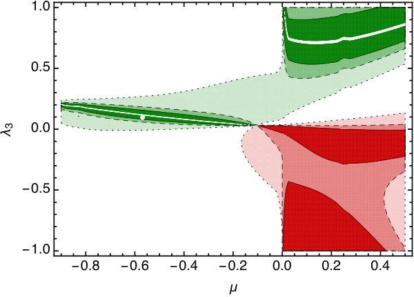
In Fig.​ 4 we show the regions in the $(\mu,\lambda_{3})$-plane where effective universality is realised for the coupling $G_{(3,0)}$ and $G_{(1,2)}$. In particular we display the regions in which $\varepsilon<\frac{1}{5}$ and $\varepsilon<\frac{1}{3}$ for $N_{s}=1$ and $G\to 0$. We further distinguish between regions that allow for a UV fixed point ($\Delta\beta<0$, green colour) and regions that do not ($\Delta\beta>0$, red colour). We observe that effective universality and a UV fixed point is only allowed in two regions: this first is for negative $\mu$ and small $\lambda_{3}\approx 0.1$. In fact our fixed-point values for $\mu$ and $\lambda_{3}$ lie in this region of effective universality. In Fig.​ 4 it is marked by a white dot. The other region is at positive $\mu$ and large $\lambda_{3}>0.5$. At positive $\mu$ and negative $\lambda_{3}$ there is another region that allows for effective universality but not for a UV fixed point at positive Newton coupling. Fig.​ 4 highlights that the common realisation of effective universality and a UV fixed point is highly non-trivial.

As effective universality is restored exactly at the fixed point, i.e. if $\mu$ and $\lambda$ are set to their fixed-point values in $\beta_{G_{(3,0)}}$ and $\beta_{G_{(1,2)}}$, the critical exponents do not reflect effective universality: the real parts of the relevant critical exponents actually feature distinct dependencies on $N_{s}$, cf. Fig.​ 5. In particular, the eigendirection which has most overlap with $G_{(1,2)}$ increases in relevance for increasing $N_{s}$. On the other hand, two superpositions of $G_{(3,0)}$ and $\mu$ form two relevant eigendirections, both of which become less relevant as $N_{s}$ is increased.

It is useful to investigate in which commonly used approximation effective universality survives. We have already observed that in our truncation a derivative expansion spoils effective universality for the $N_{s}$-independent part, cf. Fig.​ 2, and it also does not hold anymore away from the fixed point, cf. Fig.​ 4. We now take a closer look at the $N_{s}$-dependent part, where from the left panel of Fig.​ 3 we already infer that a derivative expansion works rather well.

At $\mu=0=\lambda_{3}$ and evaluated with a derivative expansion at $p^{2}=0$, the flow equations for the dynamical Newton couplings are given by the analytic expressions

	$\displaystyle\beta_{G_{(3,0)}}=(2+$	$\displaystyle 3\eta_{h})G_{(3,0)}-\frac{833}{285\pi}G_{(3,0)}^{2}$
		$\displaystyle-\frac{43}{570\pi}N_{s}\,G_{(3,0)}^{1/2}G_{(1,2)}^{3/2}\,,$
	$\displaystyle\beta_{G_{(1,2)}}=(2+$	$\displaystyle\eta_{h}+2\eta_{\varphi})G_{(1,2)}$
		$\displaystyle-\frac{4}{\pi}G_{(1,2)}^{2}+\frac{8}{3\pi}G_{(3,0)}^{1/2}G_{(1,2)}^{3/2}\,,$		(31)

where we again identified $G_{(n\geq 3,0)}=G_{(3,0)}$ and $G_{(n,m\geq 2)}=G_{(1,2)}$ and set the anomalous dimension on the right-hand side of the Wetterich equation to zero. The graviton anomalous dimension in the canonical term gives a leading-order contribution and thus we need to include its $N_{s}$-dependence. With a projection at $p^{2}=0$ the contribution is

$\displaystyle\eta_{h}\Big|_{N_{s}}=\frac{1}{24\pi}N_{s}\,G_{(1,2)}\,.$

(32)

A projection at finite momentum changes the size of the contribution but not the sign. The scalar anomalous dimension does not have any $N_{s}$-dependence. We use this together with (31) and find

	$\displaystyle\beta_{G_{(3,0)}}\Big|_{N_{s}}$	$\displaystyle\approx 0.016\,G^{2}N_{s}\,,$
	$\displaystyle\beta_{G_{(1,2)}}\Big|_{N_{s}}$	$\displaystyle\approx 0.013\,G^{2}N_{s}\,.$		(33)

Note that all the above $N_{s}$-dependent contributions are gauge independent as they originate from scalar loops. We find a good agreement between the two fluctuation couplings $\beta_{G_{(3,0)}}|_{N_{s}}$ and $\beta_{G_{(1,2)}}|_{N_{s}}$, having only a 16% deviation of their coefficients.

References

- [1] S. Weinberg, General Relativity: An Einstein centenary survey, Eds. Hawking, S.W., Israel, W; Cambridge University Press , 790 (1979).
- [2] M. Reuter, Phys. Rev. D57, 971 (1998), arXiv:hep-th/9605030 .
- [3] N. Christiansen, D. F. Litim, J. M. Pawlowski, and A. Rodigast, Phys.Lett. B728, 114 (2014), arXiv:1209.4038 [hep-th] .
- [4] N. Christiansen, B. Knorr, J. M. Pawlowski, and A. Rodigast, Phys. Rev. D93, 044036 (2016), arXiv:1403.1232 [hep-th] .
- [5] N. Christiansen, B. Knorr, J. Meibohm, J. M. Pawlowski, and M. Reichert, Phys. Rev. D92, 121501 (2015), arXiv:1506.07016 [hep-th] .
- [6] T. Denz, J. M. Pawlowski, and M. Reichert, Eur. Phys. J. C78, 336 (2018), arXiv:1612.07315 [hep-th] .
- [7] J. Meibohm, J. M. Pawlowski, and M. Reichert, Phys. Rev. D93, 084035 (2016), arXiv:1510.07018 [hep-th] .
- [8] P. Donà, A. Eichhorn, P. Labus, and R. Percacci, Phys. Rev. D93, 044049 (2016), [Erratum: Phys. Rev.D93,no.12,129904(2016)], arXiv:1512.01589 [gr-qc] .
- [9] A. Eichhorn, S. Lippoldt, and V. Skrinjar, Phys. Rev. D97, 026002 (2018a), arXiv:1710.03005 [hep-th] .
- [10] N. Christiansen, D. F. Litim, J. M. Pawlowski, and M. Reichert, Phys. Rev. D97, 106012 (2018a), arXiv:1710.04669 [hep-th] .
- [11] B. Knorr and S. Lippoldt, Phys. Rev. D96, 065020 (2017), arXiv:1707.01397 [hep-th] .
- [12] N. Christiansen, K. Falls, J. M. Pawlowski, and M. Reichert, Phys. Rev. D97, 046007 (2018b), arXiv:1711.09259 [hep-th] .
- [13] B. Knorr, Class. Quant. Grav. 35, 115005 (2018), arXiv:1710.07055 [hep-th] .
- [14] E. Manrique and M. Reuter, Annals Phys. 325, 785 (2010), arXiv:0907.2617 [gr-qc] .
- [15] E. Manrique, M. Reuter, and F. Saueressig, Annals Phys. 326, 440 (2011a), arXiv:1003.5129 [hep-th] .
- [16] E. Manrique, M. Reuter, and F. Saueressig, Annals Phys. 326, 463 (2011b), arXiv:1006.0099 [hep-th] .
- [17] D. Becker and M. Reuter, Annals Phys. 350, 225 (2014a), arXiv:1404.4537 [hep-th] .
- [18] M. Reuter and H. Weyer, Phys. Rev. D79, 105005 (2009a), arXiv:0801.3287 [hep-th] .
- [19] M. Reuter and H. Weyer, Phys. Rev. D80, 025001 (2009b), arXiv:0804.1475 [hep-th] .
- [20] I. Donkin and J. M. Pawlowski, (2012), arXiv:1203.4207 [hep-th] .
- [21] J. A. Dietz and T. R. Morris, JHEP 04, 118 (2015), arXiv:1502.07396 [hep-th] .
- [22] M. Safari, Eur. Phys. J. C76, 201 (2016), arXiv:1508.06244 [hep-th] .
- [23] P. Labus, T. R. Morris, and Z. H. Slade, Phys. Rev. D94, 024007 (2016a), arXiv:1603.04772 [hep-th] .
- [24] T. R. Morris, JHEP 11, 160 (2016), arXiv:1610.03081 [hep-th] .
- [25] R. Percacci and G. P. Vacca, Eur. Phys. J. C77, 52 (2017), arXiv:1611.07005 [hep-th] .
- [26] N. Ohta, PTEP 2017, 033E02 (2017), arXiv:1701.01506 [hep-th] .
- [27] C. M. Nieto, R. Percacci, and V. Skrinjar, Phys. Rev. D96, 106019 (2017), arXiv:1708.09760 [gr-qc] .
- [28] O. Lauscher and M. Reuter, Phys. Rev. D65, 025013 (2002a), arXiv:hep-th/0108040 .
- [29] M. Reuter and F. Saueressig, Phys. Rev. D65, 065016 (2002), arXiv:hep-th/0110054 [hep-th] .
- [30] O. Lauscher and M. Reuter, Phys. Rev. D66, 025026 (2002b), arXiv:hep-th/0205062 .
- [31] D. F. Litim, Phys.Rev.Lett. 92, 201301 (2004), arXiv:hep-th/0312114 [hep-th] .
- [32] P. Fischer and D. F. Litim, Phys.Lett. B638, 497 (2006), arXiv:hep-th/0602203 [hep-th] .
- [33] A. Codello and R. Percacci, Phys. Rev. Lett. 97, 221301 (2006), arXiv:hep-th/0607128 .
- [34] P. F. Machado and F. Saueressig, Phys. Rev. D77, 124045 (2008), arXiv:0712.0445 [hep-th] .
- [35] A. Codello, R. Percacci, and C. Rahmede, Annals Phys. 324, 414 (2009), arXiv:0805.2909 [hep-th] .
- [36] D. Benedetti, P. F. Machado, and F. Saueressig, Mod. Phys. Lett. A24, 2233 (2009), arXiv:0901.2984 [hep-th] .
- [37] A. Eichhorn, H. Gies, and M. M. Scherer, Phys. Rev. D80, 104003 (2009), arXiv:0907.1828 [hep-th] .
- [38] A. Eichhorn and H. Gies, Phys. Rev. D81, 104010 (2010), arXiv:1001.5033 [hep-th] .
- [39] K. Groh and F. Saueressig, J. Phys. A43, 365403 (2010), arXiv:1001.5032 [hep-th] .
- [40] E. Manrique, S. Rechenberger, and F. Saueressig, Phys.Rev.Lett. 106, 251302 (2011c), arXiv:1102.5012 [hep-th] .
- [41] D. Benedetti and F. Caravelli, JHEP 06, 017 (2012), [Erratum: JHEP10,157(2012)], arXiv:1204.3541 [hep-th] .
- [42] J. A. Dietz and T. R. Morris, JHEP 01, 108 (2013), arXiv:1211.0955 [hep-th] .
- [43] K. Falls, D. Litim, K. Nikolakopoulos, and C. Rahmede, (2013), arXiv:1301.4191 [hep-th] .
- [44] A. Codello, G. D’Odorico, and C. Pagani, Phys. Rev. D89, 081701 (2014), arXiv:1304.4777 [gr-qc] .
- [45] K. Falls, D. F. Litim, K. Nikolakopoulos, and C. Rahmede, Phys. Rev. D93, 104022 (2016), arXiv:1410.4815 [hep-th] .
- [46] D. Becker and M. Reuter, JHEP 12, 025 (2014b), arXiv:1407.5848 [hep-th] .
- [47] K. Falls, Phys. Rev. D92, 124057 (2015a), arXiv:1501.05331 [hep-th] .
- [48] A. Eichhorn, JHEP 04, 096 (2015), arXiv:1501.05848 [gr-qc] .
- [49] K. Falls, (2015b), arXiv:1503.06233 [hep-th] .
- [50] M. Demmel, F. Saueressig, and O. Zanusso, JHEP 08, 113 (2015), arXiv:1504.07656 [hep-th] .
- [51] H. Gies, B. Knorr, and S. Lippoldt, Phys. Rev. D92, 084020 (2015), arXiv:1507.08859 [hep-th] .
- [52] H. Gies, B. Knorr, S. Lippoldt, and F. Saueressig, Phys. Rev. Lett. 116, 211302 (2016), arXiv:1601.01800 [hep-th] .
- [53] N. Ohta, R. Percacci, and A. D. Pereira, JHEP 06, 115 (2016), arXiv:1605.00454 [hep-th] .
- [54] J. Biemans, A. Platania, and F. Saueressig, Phys. Rev. D95, 086013 (2017a), arXiv:1609.04813 [hep-th] .
- [55] N. Ohta, R. Percacci, and A. D. Pereira, Eur. Phys. J. C77, 611 (2017), arXiv:1610.07991 [hep-th] .
- [56] N. Christiansen, (2016), arXiv:1612.06223 [hep-th] .
- [57] K. Falls, Phys. Rev. D96, 126016 (2017), arXiv:1702.03577 [hep-th] .
- [58] S. Gonzalez-Martin, T. R. Morris, and Z. H. Slade, Phys. Rev. D95, 106010 (2017), arXiv:1704.08873 [hep-th] .
- [59] C. Wetterich, Phys. Lett. B773, 6 (2017), arXiv:1704.08040 [gr-qc] .
- [60] S. P. de Alwis, JHEP 03, 118 (2018), arXiv:1707.09298 [hep-th] .
- [61] K. Falls, C. R. King, D. F. Litim, K. Nikolakopoulos, and C. Rahmede, Phys. Rev. D97, 086006 (2018), arXiv:1801.00162 [hep-th] .
- [62] C. Wetterich, (2018), arXiv:1802.05947 [gr-qc] .
- [63] A. Eichhorn and A. Held, (2018), arXiv:1803.04027 [hep-th] .
- [64] D. Dou and R. Percacci, Class. Quant. Grav. 15, 3449 (1998), arXiv:hep-th/9707239 [hep-th] .
- [65] R. Percacci and D. Perini, Phys. Rev. D67, 081503 (2003a), arXiv:hep-th/0207033 .
- [66] R. Percacci and D. Perini, Phys. Rev. D68, 044018 (2003b), arXiv:hep-th/0304222 .
- [67] G. Narain and R. Percacci, Class. Quant. Grav. 27, 075001 (2010), arXiv:0911.0386 [hep-th] .
- [68] A. Eichhorn, Phys. Rev. D86, 105021 (2012), arXiv:1204.0965 [gr-qc] .
- [69] T. Henz, J. M. Pawlowski, A. Rodigast, and C. Wetterich, Phys. Lett. B727, 298 (2013), arXiv:1304.7743 [hep-th] .
- [70] P. Donà, A. Eichhorn, and R. Percacci, Phys.Rev. D89, 084035 (2014), arXiv:1311.2898 [hep-th] .
- [71] R. Percacci and G. P. Vacca, Eur. Phys. J. C75, 188 (2015), arXiv:1501.00888 [hep-th] .
- [72] P. Labus, R. Percacci, and G. P. Vacca, Phys. Lett. B753, 274 (2016b), arXiv:1505.05393 [hep-th] .
- [73] K.-y. Oda and M. Yamada, Class. Quant. Grav. 33, 125011 (2016), arXiv:1510.03734 [hep-th] .
- [74] T. Henz, J. M. Pawlowski, and C. Wetterich, Phys. Lett. B769, 105 (2017), arXiv:1605.01858 [hep-th] .
- [75] C. Wetterich and M. Yamada, Phys. Lett. B770, 268 (2017), arXiv:1612.03069 [hep-th] .
- [76] J. Biemans, A. Platania, and F. Saueressig, JHEP 05, 093 (2017b), arXiv:1702.06539 [hep-th] .
- [77] Y. Hamada and M. Yamada, JHEP 08, 070 (2017), arXiv:1703.09033 [hep-th] .
- [78] D. Becker, C. Ripken, and F. Saueressig, JHEP 12, 121 (2017), arXiv:1709.09098 [hep-th] .
- [79] A. Eichhorn, Y. Hamada, J. Lumma, and M. Yamada, Phys. Rev. D97, 086004 (2018b), arXiv:1712.00319 [hep-th] .
- [80] N. Alkofer and F. Saueressig, (2018), arXiv:1802.00498 [hep-th] .
- [81] M. Niedermaier, Class. Quant. Grav. 24, R171 (2007), arXiv:gr-qc/0610018 .
- [82] D. F. Litim, Phil.Trans.Roy.Soc.Lond. A369, 2759 (2011), arXiv:1102.4624 [hep-th] .
- [83] M. Reuter and F. Saueressig, New J. Phys. 14, 055022 (2012), arXiv:1202.2274 [hep-th] .
- [84] A. Bonanno and F. Saueressig, Comptes Rendus Physique 18, 254 (2017), arXiv:1702.04137 [hep-th] .
- [85] R. Percacci, An Introduction to Covariant Quantum Gravity and Asymptotic Safety, 100 Years of General Relativity, Vol. 3 (World Scientific, 2017).
- [86] A. Eichhorn, in Black Holes, Gravitational Waves and Spacetime Singularities Rome, Italy, May 9-12, 2017 (2017) arXiv:1709.03696 [gr-qc] .
- [87] U. Ellwanger, M. Hirsch, and A. Weber, Z.Phys. C69, 687 (1996), arXiv:hep-th/9506019 [hep-th] .
- [88] A. K. Cyrol, M. Mitter, J. M. Pawlowski, and N. Strodthoff, Phys. Rev. D97, 054006 (2018), arXiv:1706.06326 [hep-ph] .
- [89] M. M. Anber and J. F. Donoghue, Phys. Rev. D85, 104016 (2012), arXiv:1111.2875 [hep-th] .
- [90] C. Wetterich, Phys. Lett. B301, 90 (1993), arXiv:1710.05815 [hep-th] .
- [91] U. Ellwanger, Proceedings, Workshop on Quantum field theoretical aspects of high energy physics: Bad Frankenhausen, Germany, September 20-24, 1993, Z. Phys. C62, 503 (1994), arXiv:hep-ph/9308260 [hep-ph] .
- [92] T. R. Morris, Int. J. Mod. Phys. A9, 2411 (1994), arXiv:hep-ph/9308265 .
- [93] A. Eichhorn, Phys. Rev. D87, 124016 (2013), arXiv:1301.0632 [hep-th] .
- [94] M. Reuter and C. Wetterich, Nucl. Phys. B417, 181 (1994).
- [95] J. F. Donoghue, Phys. Rev. Lett. 72, 2996 (1994), arXiv:gr-qc/9310024 .
- [96] S. P. Robinson and F. Wilczek, Phys. Rev. Lett. 96, 231601 (2006), arXiv:hep-th/0509050 .
- [97] A. R. Pietrykowski, Phys. Rev. Lett. 98, 061801 (2007), arXiv:hep-th/0606208 .
- [98] D. J. Toms, Phys. Rev. D76, 045015 (2007), arXiv:0708.2990 [hep-th] .
- [99] D. Ebert, J. Plefka, and A. Rodigast, Phys. Lett. B660, 579 (2008), arXiv:0710.1002 [hep-th] .
- [100] A. Rodigast and T. Schuster, Phys. Rev. Lett. 104, 081301 (2010), arXiv:0908.2422 [hep-th] .
- [101] E. Álvarez, S. González-Martín, M. Herrero-Valea, and C. P. Martín, JHEP 08, 078 (2015), arXiv:1505.01995 [hep-th] .
- [102] D. F. Litim and J. M. Pawlowski, Phys.Lett. B435, 181 (1998), arXiv:hep-th/9802064 [hep-th] .
- [103] J. J. W. York, J. Math. Phys. 14, 456 (1973).
- [104] K. S. Stelle, Phys. Rev. D16, 953 (1977).
- [105] J. A. M. Vermaseren, (2000), arXiv:math-ph/0010025 [math-ph] .
- [106] J. Kuipers, T. Ueda, J. A. M. Vermaseren, and J. Vollinga, Comput. Phys. Commun. 184, 1453 (2013), arXiv:1203.6543 [cs.SC] .
- [107] A. K. Cyrol, M. Mitter, and N. Strodthoff, Comput. Phys. Commun. 219, 346 (2017), arXiv:1610.09331 [hep-ph] .
- [108] J. Meibohm and J. M. Pawlowski, Eur. Phys. J. C76, 285 (2016), arXiv:1601.04597 [hep-th] .
- [109] D. F. Litim, Phys.Lett. B486, 92 (2000), arXiv:hep-th/0005245 [hep-th] .
- [110] D. F. Litim, Phys.Rev. D64, 105007 (2001), arXiv:hep-th/0103195 [hep-th] .
- [111] D. F. Litim and J. M. Pawlowski, JHEP 0209, 049 (2002a), arXiv:hep-th/0203005 [hep-th] .
- [112] D. F. Litim and J. M. Pawlowski, Phys.Lett. B546, 279 (2002b), arXiv:hep-th/0208216 [hep-th] .
- [113] J. M. Pawlowski, (2003), arXiv:hep-th/0310018 [hep-th] .
- [114] J. M. Pawlowski, http://www.thphys.uni-heidelberg.de/~pawlowski/FRG/literature/review.pdf.
- [115] J. M. Pawlowski, Annals Phys. 322, 2831 (2007), arXiv:hep-th/0512261 [hep-th] .
- [116] I. Donkin, Diploma thesis, Heidelberg (2008).
- [117] I. H. Bridle, J. A. Dietz, and T. R. Morris, JHEP 03, 093 (2014), arXiv:1312.2846 [hep-th] .
- [118] M. Reuter and C. Wetterich, Phys.Rev. D56, 7893 (1997), arXiv:hep-th/9708051 [hep-th] .
- [119] U. Reinosa, J. Serreau, M. Tissier, and N. Wschebor, Phys. Lett. B742, 61 (2015), arXiv:1407.6469 [hep-ph] .