Economical and efficient network super points detection based on GPU

Suppose there are two networks: $NT_{a}$ and $NT_{b}$. Let $A$ and $B$ represent the hosts set of these two networks. $NT_{a}$ and $NT_{b}$ communicate with each other by a group of edge routers as shown in figure 1. These routers compose the edge of $NT_{a}$ and $NT_{b}$, written as $E(a,b)$. Through $E(a,b)$ we can observe packets stream in two directions: from $NT_{a}$ to $NT_{b}$ and from $NT_{b}$ to $NT_{a}$. For a host $a_{0}$ in $NT_{a}$, the task of cardinality estimation is to get the number of hosts in $NT_{b}$ that communicate with $a_{0}$ in a certain time period. "communicate" means send packets to or receive packets from $a_{0}$. Let $CO(a_{0})$ represent the set of these hosts. Calculate $a_{0}$’s cardinality is to find the number of elements in $CO(a_{0})$, written as $|CO(a_{0})|$. Because a host in $CO(a_{0})$ may have several packets communicating with $a_{0}$, we should find out the number of distinct hosts from packets stream. Super point is a host whose cardinality is more than a certain threshold $\theta$. After getting hosts’ cardinalities, we can filter super points easily.

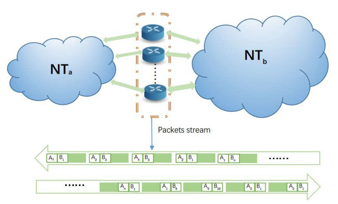
WHANG et al (18) gives a simple way to estimate the distinct number from data stream, called linear estimator. We use linear estimator to calculate host’s cardinality. At the beginning, a bit vector with $g$ zero bits is allocated. When scanning a packet with a host $b_{0}$ in $NT_{b}$ and $a_{0}$ in $NT_{a}$ at $E(a,b)$, we set a random bit to 1. This bit is select by $b_{0}$’s hashed value with a random hash function $H_{1}$(19). After scanning all packets in a time period, we can report the estimating cardinality $Est^{\prime}$ by the follow equation:

$z_{0}$ is the number of zero bits remaining at the end of the time period. We call this algorithm as linear estimator.

Linear estimator uses fixed number of bits and has a fast processing speed because for every packet it only needs to access memory once. But in a high speed network, it’s too expensive to allocate a linear estimator for every host because of the following reasons.

1. (1)

   Memory requirement. There are huge hosts in high speed network. Allocating a linear estimator for every host requires great memory. For example, when $g$ is set to 1024, and there are 8 million hosts in $NT_{a}$, 1 GB memory is desired. Allocating or transmitting such huge memory between different edge routers is a heavy burden.

2. (2)

   Linear estimator locating. These hosts in a network may have discrete addresses and we can’t locate their linear estimators directly by their IP addresses. In order to find a host’s linear estimator, we have to use hash table or balance tree to store these linear estimators. But hash table has collision problems(20) and balance tree requires additional memory accessing(21).

To solve this problem, we design a novel structure which can detect super points and estimate their cardinalities using fixed number of linear estimators. We will introduce our novel algorithm in detail in the following part.

Because it is low efficient that a linear estimator is used by a host exclusive, we let a linear estimator can be shared by several hosts. Let $LA^{g,k}$ represent an array of $2^{k}$ estimators with $g$ bits in each one. Every host will select a linear estimator from $LA^{g,k}$ to estimator its cardinality.

But this will cause a higher estimation value than the real cardinality. In order to reduce the effect of sharing linear estimator, we use $r$ $LA^{g,k}$s together and each host will select $r$ linear estimators from every $LA^{g,k}$ to record its cardinality at the same time as described in figure 2

For a host $a_{0}$ in $NT_{a}$, let $LE(a_{0})$ represent the set linear estimators in these $r$ $LA^{g,k}$s that used to record $a_{0}$’s cardinality. At the end of a time period, we will calculate the union linear estimator $ULE(a_{0})$ by applying bit-wise "AND" operation to all linear estimators in $LE(a_{0})$ and get $a_{0}$’s estimating value from $ULE(a_{0})$.

In order to get a high accuracy estimation value and detect super points from these $r$ $LA$, how to select linear estimators in different $LA^{g,k}$ should comply with the following two requirements:

1. (1)

   Each estimator in $LA$ should have the same probability to be used by different hosts. This will make sure that every linear estimator is fully utilized and the algorithm can acquire the highest accuracy with the smallest memory.

2. (2)

   For a super point $a_{0}$, we can reconstruct it from $LE(a_{0})$. At the end of a time period, all what we have are $r$ $LA^{g,k}$s that record all hosts’ cardinalities. Super points will be reconstructed from all of these $LA^{g,k}$s.

The key to these requirements is how to map a host to $r$ linear estimators in $LA$( in the rest of this paper, we use $LA$ to represent $LA^{g,k}$ simply). We devise a novel double direction hash functions group, written as $DHG$, which contains $r$ random hash functions. $DHG$ can hash an integer $i$ to $r$ random values between 0 and $2^{k}-1$ where $i$ and $k$ are both positive integers. What’s more, $i$ could be restored from its hashed $r$ values. We can use equation 1 to find out which linear estimator’s estimating value is more than $\theta$ and we call this kind of estimator as hot estimator. When $a_{0}$ is a super point, $LE(a_{0})$ will appear in hot estimators. By $DHG$, we can restore $a_{0}$ from $LE(a_{0})$.

The first hash function $DH_{0}$ in $DHG$ is a random hash function(19) that maps a host $a_{0}$ to a value between 0 and $2^{k}-1$ uniformly. $DH_{0}$ has excellent randomness, but it requires great operations and is not reversible. For the sake of super point reconstruction and randomness, the rest $r-1$ hash functions are determined by the following equation:

$\alpha$ is a positive integer, "$>>$"is bitwise right shift operation and $\bigoplus$ is a bitwise "exclusive or" operation. $DH_{0}(a_{0})$ is a random seed which makes sure all the $r$ hash functions has a high randomness. Because $k$ is a positive integer, $(a_{0}>>(i-1)*\alpha))mod(2^{k})$ is successive $k$ bits of $a_{0}$ starting from $(i-1)*\alpha$. We call these bits as bit block, written as $BL(i)$. $BL(i)$ could be restored from $DH_{i}(a_{0})$ by equation 3.

If $BL(i)$ is long enough, we can reconstruct $a_{0}$ by concatenating these $r-1$ $BL$s. We call these $r$ $LA$s hashing by $DHG$ as Double direction Hash Linear estimators Array $DHLA$. Algorithm 1 shows how to scan packets and update $DHLA$.

Algorithm 1 has very little operations which let it have a fast processing speed for core network which forwards millions of packets every second. $DHLA$ maintains all hosts’ cardinalities and when $\alpha$ and $r$ is reasonably selected, super points could be restored efficiently. In the next part, how to restore super points from $DHLA$ will be discussed in detail.

$BL(i)$ is a fraction of $a_{0}$. If every bit of $a_{0}$ is contained in some $BL(i)$, $a_{0}$ could be reconstructed entirely. Figure 3 illustrates the relationship between $a_{0}$ and $BL(i)$.

In order to reconstruct $a_{0}$, $r$ $\alpha$ and $k$ should comply with the following two restrictions:

1. (1)

   $\alpha\leq k$. This makes sure that there are no missing bits between two neighboring $BL$s. When $0<\alpha<k$, there will be $k-\alpha$ bits be the same in two neighboring $BL$s. These duplicating bits will help us to filter candidate IP from $DHLA$.

2. (2)

   $(r-2)*\alpha+k\geq 32$. This restriction means that the last $BL$ will contains the last bit of $a_{0}$.

When these two conditions are met, $a_{0}$ could be restored from these $r-1$ $BL$s by comparing and concatenating operations and $BL(i)$ could be acquired by equation 3.

But do not store $LE(a_{0})$ when scanning packets, we can’t get $BL(i)$ directly. According to the definition of super points, when $a_{0}$ is a super point, each linear estimator in $LE(a_{0})$ is a hot estimator. We can first find out all hot estimators in every $LA$ and then test them one by one to restore super points. After getting $a_{0}$, we can get $ULE(a_{0})$ and estimate $a_{0}$’s cardinality according to the zero number in $ULE(a_{0})$. But equation 1 could not be used here directly because some bits of $ULE(a_{0})$ may be set by other hosts. In order to get a high accuracy result, we should estimate the number of "1" bits set by other hosts and remove them. The following lemma and theorem show how to do this. Flow in this paper means the set of packets with the same IP addresses.

$w$ could be estimated by equation 1 from every $LA$ because $LA$ could be regarded as a bit set used to record the flow number. We can get the "0" bit number $ZR(i)$ of the $i$th $LA$, and estimate the flow number ${w(i)}^{\prime}$ from it ${w(i)}^{\prime}=-g*2^{k}*ln(\frac{ZR(i)}{g*2^{k}})$. We use the average value of all the $r$ estimating value of every $LA$ as the flow number ${w}^{\prime}=\frac{\sum_{i=0}^{r-1}{w(i)}^{\prime}}{r}$.

In $LA$, several hosts may be mapped to the same linear estimator. It causes that the "0" bit number of $ULE(a_{0})$ is smaller than that when the linear estimators are used by $a_{0}$ exclusively.

In theorem 3.3, $SZ(a_{0})$ is the zero number in $ULE(a_{0})$. $a_{0}$’s cardinality $C(a_{0})$ could be estimated from $EZ(a_{0})$ by the following equation:

Algorithm 2 shows how to detect super points from $DHLA$ and estimate their cardinalities.

In algorithm 2, $LA(i,j)$ points to the $j$th linear estimator in the $i$ $LA$. The weight of $LA(i,j)$, written as $|LA(i,j)|$ is the number of "1"bits in it.

Both algorithm 1 and 2 have no data conflict which make sure that we can launch them on several threads concurrence to get a high processing speed. In the next section, we will introduce how to deploy our super points detection algorithm on GPU.

From each edge router, we can monitor a packet stream and extract IP address pairs from this stream. Super points will be detected from IP address pairs. Packets could be mirrored to a monitor sever alongside a router. If we want to use GPU to scan IP address pairs, we have to copy them from monitor server’s memory to GPU’s global memory. An IP address pair is a vector of two IP addresses extracting from a packet. It is low efficient to copy every IP address pair one by one because the coping procedure requires additional starting and ending operations. We allocate a IP address buffer on both monitor server and GPU. This IP pair buffer could store $\mu$ IP pairs and its size is $8*\mu$ bytes. Figure 4 illustrates how to scan IP pairs on monitor server. When monitor server receives packets from router, it will extract IP pairs and store them to IP pair buffer on its memory. When the IP buffer has stored $\mu$ IP pairs, server monitor will copy it to GPU buffer. GPU card is locating on monitor server’s board connecting it with PCIe3.0 bus. After copying to GPU, monitor server’s buffer will be cleared for storing another $\mu$ IP pairs. When receiving $\mu$ IP pairs from monitor server, GPU will launch $\mu$ threads running algorithm 1 to process this $\mu$ IP pairs parallel. In algorithm 1, a bit could be set by several threads at the same time without mistakes. So these $\mu$ threads could update $DHLA$ parallel.

At the end of a time period, we can estimate super point cardinality from $DHLA$. If there are more than one edge routers, we can merge their local $DHLA$s to a global one by bit wise "AND" operation and use the global $DHLA$ to estimate super point cardinality. In the rest of this section, $DHLA$ means the global $DHLA$ merging from all local monitor servers.

Super point cardinality estimation could be divided into three parts: hot linear estimators identifying, super points detection, cardinality estimation. All of these parts could be implement on GPU parallel.

To get $HE(i)$, we have to count the zero bit number of every linear estimator. There are total $r*2^{k}$ linear estimators in $DHLA$. The number of linear estimators may be more than the maximum of available threads on GPU. We use a fixed number of threads to test all of these linear estimators and every thread will test more than one linear estimators. The hot linear estimator checking algorithm is very simple, counting the number of zero bits and comparing the number with a positive integer. This will not consume much time in GPU.

After getting $HE(i)$ of every $LA$, we will try to restore super points from them. In algorithm 2, select $r$ linear estimators from every $HE(i)$ to generate a hot estimator tuple and test every of this tuple one by one. This method is simple but very low efficient. Because there are $\prod_{i=0}^{r}{|HE(i)|}$ tuples, checking all of these tuples one by one will consume much time, especially when there are many super points.

Observing that if $CL_{0}\in HE_{0}$, $CL_{1}\in HE_{1}$, $CL_{2}\in HE_{2}$ and the left $k-\alpha$ bits of $CL_{0}\bigoplus CL_{1}$ not equal to the right $k-\alpha$ bits of $CL_{0}\bigoplus CL_{1}$, there is no need to check any tuples that contain $CL_{0}$ $CL_{1}$ and $CL_{2}$. So we will restore super points incrementally from $HE(1)$ to $HE(r-1)$ and store the intermediate result. But if we want to run parallel in GPU, we have to allocate two buffers for intermediate result: one for reading and the other for storing. Because $BL(i)$ depends on $DH_{0}$, in the intermediate result we will store which linear estimator is used to reconstruct $BL$ and the restored partial IP address. The first three $HE$ have different process with the others, so we will discuss them separately.

Firstly, we allocate two buffers in GPU global memory, $SubIP_{1}$ and $SubIP_{2}$, to store partial IP addresses and $DH_{0}$. The size of these buffers, $|SubIP_{1}|$ or $|SubIP_{2}|$, is the number of partial IP addresses it stores. For the first three $HE$s, there are $|HE_{0}|*|HE_{1}|*|HE_{2}|$ tuples like $<CL_{0},CL_{1},CL_{2}>$ where $CL_{i}\in HE_{i}$. Denote the set of these tuples as $TP_{<0,1,2>}$. Suppose we launch $TN$ threads on GPU to deal with $TP_{<0,1,2>}$. Let $a$, $b$ be two non-negative integers that $a*TN+b=|HE_{0}|*|HE_{1}|*|HE_{2}|$. Each of the first $b$ thread will test $a+1$ tuples and each of the rest $TN-b$ thread will check $a$ tuples. Let $TP_{<0,1,2>}(i)$ represent the set of tuples in $TP_{<0,1,2>}$ to be scanned by the $i$th thread. Algorithm 3 shows how every threads launched in GPU to deal with $TP_{<0,1,2>}$.

The roles of these two buffers may change in different stages. $SSubIP$ points to the buffer used for storing sub IP addresses in a stage and $RSubIP$ points to the buffer used for reading sub addresses. When scanning $TP_{<0,1,2>}$, $SubIP_{1}$ is used for storing sub IP addresses. After scanning $TP_{<0,1,2>}$, $SubIP_{1}$ will contain $|SubIP_{1}|$ candidate sub IP addresses. Together with $HE_{3}$, we can generate another tuples $TP_{<0,1,2,3>}$ like $<CL_{0},subip,CL_{3}>$ where $CL_{0}\in SubIP_{1}$, $subip\in SubIP_{1}$, $CL_{3}\in HE_{3}$. When scanning $TP_{<0,1,2,3>}$, $SubIP_{2}$ will be used for storing sub IP addresses, and scanning candidate partial IP addresses will be gotten from $SubIP_{1}$. Like $TP_{<0,1,2>}$, each thread will scan a sub set of $TP_{<0,1,2,3>}$. The rest $HE$ will be processed like this. $SubIP_{1}$ and $SubIP_{2}$ will play as storing buffer alternatively. Algorithm 4 shows how to scan the rest $HE$

By algorithm 4, we will restore candidate super points when scanning the last $HE$. Candidate super points are stored in a list for further checking and cardinality estimation. When dealing with $SPL$, we still start fix number of threads and each thread scans a sub set of candidate super points in $SPL$. For a candidate super point $a_{0}$, a thread will first get $ULE(a_{0})$ from $DHLA$ and count the zero bit number $z$ in it. Then $a_{0}$’s cardinality could be calculated by equation 4. If the estimating value is more than $\theta$, we will report it as a super point together with its estimating cardinality.

Because the high randomness of $DHG$, $DHLA$ requires much smaller memory than other algorithms do. So our algorithm can run on a cheap GPU to deal with high speed networks. In the next section we will give the real world traffic experiments of our algorithm comparing with several state-of-the-art algorithms.

References

- (1) Ahmed Patel, Mona Taghavi, Kaveh Bakhtiyari, and Joaquim Celestino Júnior. An intrusion detection and prevention system in cloud computing: A systematic review. Journal of Network and Computer Applications, 36(1):25 – 41, 2013.
- (2) Chirag Modi, Dhiren Patel, Bhavesh Borisaniya, Hiren Patel, Avi Patel, and Muttukrishnan Rajarajan. A survey of intrusion detection techniques in cloud. Journal of Network and Computer Applications, 36(1):42 – 57, 2013.
- (3) Hung-Jen Liao, Chun-Hung Richard Lin, Ying-Chih Lin, and Kuang-Yuan Tung. Intrusion detection system: A comprehensive review. Journal of Network and Computer Applications, 36(1):16 – 24, 2013.
- (4) Yinhui Li, Jingbo Xia, Silan Zhang, Jiakai Yan, Xiaochuan Ai, and Kuobin Dai. An efficient intrusion detection system based on support vector machines and gradually feature removal method. Expert Systems with Applications, 39(1):424 – 430, 2012.
- (5) Mansour Alsaleh and P. C. van Oorschot. Network scan detection with lqs: A lightweight, quick and stateful algorithm. In Proceedings of the 6th ACM Symposium on Information, Computer and Communications Security, ASIACCS ’11, pages 102–113, New York, NY, USA, 2011. ACM.
- (6) Richard E. Harang and Peter Mell. Evasion-resistant network scan detection. Security Informatics, 4(1):4, 2015.
- (7) J. Mirkovic, G. Prier, and P. Reiher. Attacking ddos at the source. In 10th IEEE International Conference on Network Protocols, 2002. Proceedings., pages 312–321, Nov 2002.
- (8) John Ioannidis and Steven M. Bellovin. Implementing pushback: Router-based defense against ddos attacks. In Proceedings of the Network and Distributed System Security Symposium, NDSS 2002, San Diego, California, USA, 2002.
- (9) Jelena Mirkovic and Peter Reiher. A taxonomy of ddos attack and ddos defense mechanisms. SIGCOMM Comput. Commun. Rev., 34(2):39–53, April 2004.
- (10) Shobha Venkataraman, Dawn Song, Phillip B. Gibbons, and Avrim Blum. New streaming algorithms for fast detection of superspreaders. In in Proceedings of Network and Distributed System Security Symposium (NDSS, pages 149–166, 2005.
- (11) P. Wang, X. Guan, T. Qin, and Q. Huang. A data streaming method for monitoring host connection degrees of high-speed links. IEEE Transactions on Information Forensics and Security, 6(3):1086–1098, Sept 2011.
- (12) Center for Applied Internet Data Analysis. The caida anonymized internet traces. http://www.caida.org/data/passive, 2017. Online;accessed 2017.
- (13) Guang Cheng and Yongning Tang. Line speed accurate superspreader identification using dynamic error compensation. Computer Communications, 36(13):1460 – 1470, 2013.
- (14) J. Cao, Y. Jin, A. Chen, T. Bu, and Z. L. Zhang. Identifying high cardinality internet hosts. In IEEE INFOCOM 2009, pages 810–818, April 2009.
- (15) Cristian Estan, George Varghese, and Michael Fisk. Bitmap algorithms for counting active flows on high-speed links. IEEE/ACM Trans. Netw., 14(5):925–937, October 2006.
- (16) W. Liu, W. Qu, J. Gong, and K. Li. Detection of superpoints using a vector bloom filter. IEEE Transactions on Information Forensics and Security, 11(3):514–527, March 2016.
- (17) Seon-Ho Shin, Eun-Jin Im, and MyungKeun Yoon. A grand spread estimator using a graphics processing unit. Journal of Parallel and Distributed Computing, 74(2):2039 – 2047, 2014.
- (18) Kyu-Young Whang, Brad T. Vander-Zanden, and Howard M. Taylor. A linear-time probabilistic counting algorithm for database applications. ACM Trans. Database Syst., 15(2):208–229, June 1990.
- (19) M. Naor and M. Yung. Universal one-way hash functions and their cryptographic applications. In Proceedings of the Twenty-first Annual ACM Symposium on Theory of Computing, STOC ’89, pages 33–43, New York, NY, USA, 1989. ACM.
- (20) S. Qian, J. Cao, Y. Zhu, M. Li, and J. Wang. H-tree: An efficient index structure for event matching in content-basedpublish/subscribe systems. IEEE Transactions on Parallel and Distributed Systems, 26(6):1622–1632, June 2015.
- (21) Thomas H. Cormen, Charles E. Leiserson, Ronald L. Rivest, and Clifford Stein. Introduction to Algorithms, Third Edition. The MIT Press, 3rd edition, 2009.