跳到论文正文
W Papers独立论文阅读器 arXiv:1803.11273 论文正文 计算阅读时间 · 0%
引用这篇论文根据当前论文元数据生成,正式投稿前建议核对。


License: arXiv.org perpetual non-exclusive license
arXiv:1803.11273v3 [stat.ME] 26 Jun 2019

High Dimensional Causal Discovery Under Non-Gaussianity

Y. Samuel Wang1 Address: 1Booth School of Business
University of Chicago
Chicago, IL, U.S.A.
and Mathias Drton2 Email address: ysamuelwang@gmail.com, md5@uw.edu Address: 2Department of Statistics
University of Washington
Seattle, WA, U.S.A.
Address: 2Department of Mathematical Sciences
University of Copenhagen
Copenhagen, Denmark
Abstract.

We consider graphical models based on a recursive system of linear structural equations. This implies that there is an ordering, σ\sigma, of the variables such that each observed variable YvY_{v} is a linear function of a variable specific error term and the other observed variables YuY_{u} with σ⁡(u)<σ⁡(v)\sigma(u)<\sigma(v). The causal relationships, i.e., which other variables the linear functions depend on, can be described using a directed graph. It has been previously shown that when the variable specific error terms are non-Gaussian, the exact causal graph, as opposed to a Markov equivalence class, can be consistently estimated from observational data. We propose an algorithm that yields consistent estimates of the graph also in high-dimensional settings in which the number of variables may grow at a faster rate than the number of observations, but in which the underlying causal structure features suitable sparsity; specifically, the maximum in-degree of the graph is controlled. Our theoretical analysis is couched in the setting of log-concave error distributions.

1. Introduction

Prior work shows the possibility of causal discovery with observational data in the framework of linear structural equation models with non-Gaussian errors. However, existing methods for estimation of the causal structure are applicable only in low-dimensional settings, in which the number of variables, pp, is small compared to the sample size, nn. In this paper, we develop a method which, given suitable sparsity, recovers the exact causal structure consistently in high-dimensional regimes where pp grows along with nn. Careful considerations of computational aspects make our method a practical and statistically sound exploratory tool for the intended high-dimensional settings.

Let Y1,…,Yn∈ℝpY_{1},\dots,Y_{n}\in\mathbb{R}^{p} be multivariate data from an observational study, specifically, the observations form an independent, identically distributed sample. We encode the causal structure generating dependences in the underlying pp-variate joint distribution by a graph G=(V,E)G=(V,E) with vertex set V={1,…,p}V=\{1,\dots,p\}. Each node, v∈Vv\in V, corresponds to an observed variable in Yi=(Yv​i)v∈VY_{i}=(Y_{vi})_{v\in V}, and each directed edge, (u,v)∈E(u,v)\in E, indicates that Yu​iY_{ui} has a direct causal effect on Yv​iY_{vi}. Thus, positing causal structure is equivalent to selecting a graph. We will only consider directed acyclic graphs (DAGs), directed graphs which do not contain directed cycles. Given the correspondence between a node v∈Vv\in V and the random variable Yv​iY_{vi}, we will at times let vv stand in for Yv​iY_{vi}; for instance, when stating stochastic independence relations.

Discovery of causal structure from observational data is difficult because of the super-exponential set of possible models, some of which may be indistinguishable from others. Despite this difficulty, many methods for causal discovery have been developed and have seen fruitful applications; see the recent review of Drton and Maathuis, (2017). In particular, the celebrated PC algorithm (Spirtes et al.,, 2000) is a constraint-based method which first infers a set of conditional independence relationships and then identifies the associated Markov equivalence class; this class contains all DAGs compatible with the inferred conditional independences. Kalisch and Bühlmann, (2007) show if the maximum total degree of the graph is controlled and the data is Gaussian, then the PC algorithm can consistently recover the true Markov equivalence class even in high-dimensional settings where the number of variables grows with the number of samples. Harris and Drton, (2013) extend the result to Gaussian copula models using rank correlations.

However, graphs within the same Markov equivalence class may have drastically different causal and scientific interpretations. For the graphs in Figure 1, conditional independence tests can distinguish model (a) from the rest but cannot distinguish models (b), (c), and (d) from each other. Although Maathuis et al., (2009) provide a procedure for bounding the size of a causal effect over graphs within an equivalence class, interpretation of the set of possibly conflicting graphs can remain difficult. Results on the size and number of Markov equivalence classes, which may be exponentially large, can be found e.g. in Steinsky, (2013).

123
(a)
123
(b)
123
(c)
123
(d)
Figure 1. The Markov equivalence class of graph (a) is a singleton. However, graph (b), (c) and (d) are Markov equivalent and imply the same set of conditional independences.

In contrast, it has been shown that under various additional assumptions, the exact graph structure, not just an equivalence class, can be identified from observational data (Loh and Bühlmann,, 2014; Peters and Bühlmann,, 2014; Rothenhäusler et al.,, 2018). In particular, Shimizu et al., (2006) show this to be the case under three main assumptions: (1) the data are generated by a linear structural equation model, (2) the error terms in the structural equations are non-Gaussian, and (3) there is no unobserved confounding among the observed variables; i.e., errors are independent. These assumptions yield the linear non-Gaussian acyclic model, abbreviated as LiNGAM, which is described formally in Section 2.1. Under the LiNGAM framework, the four models from Figure 1 are mutually distinguishable. Shimizu et al., (2006) use independent component analysis to estimate the graph structure, and the subsequent DirectLINGAM (Shimizu et al.,, 2011) and Pairwise LiNGAM (Hyvärinen and Smith,, 2013) methods iteratively select a causal ordering by computing pairwise statistics. These methods are motivated by identifiability results that are derived by iteratively forming conditional expectations. In practice, the conditional expectations are estimated using larger and larger regression models. As a result, the methods become inapplicable when the number of variables exceeds the sample size.

We develop a modification of the DirectLiNGAM algorithm that is suitable for high-dimensional data and give guarantees for when our algorithm will consistently recover the true graph in high-dimensional asymptotic scenarios. Most notably, our analysis considers restricted maximum in-degree of the graph and assumes log-concave distributions. The theory also applies to hub graphs where the maximum out-degree may grow with the size of the graph, which is in contrast to the conditions needed for high-dimensional consistency of the PC algorithm (Kalisch and Bühlmann,, 2007). Hub graphs appear in many biological networks (Hao et al.,, 2012).

2. Causal discovery algorithm

2.1. Generative model and notation

We assume that the observations Y1,…,Yn∈ℝpY_{1},\ldots,Y_{n}\in\mathbb{R}^{p} are independent, identically distributed replications generated from a linear structural equation model so that the elements of each random vector YiY_{i} satisfy

(1) Yv​i=∑u≠vβv​u​Yu​i+εv​i,Y_{vi}=\sum_{u\neq v}\beta_{vu}Y_{ui}+\varepsilon_{vi},

where the βv​u\beta_{vu} are unknown real parameters that quantify the direct linear effect of variable uu on variable vv, and εv​i\varepsilon_{vi} is an error term of unknown distribution PvP_{v}. We assume εv​i\varepsilon_{vi} has mean 0 and is independent of all other error terms. Our interest is in models that postulate that a particular set of coefficients βv​u\beta_{vu} is zero. In particular, the absence of an edge, (u,v)∉E(u,v)\notin E, indicates that the model constrains the parameter βv​u\beta_{vu} to zero. We assume that the graph, GG, representing the model is a DAG, which implies that the structural equation model is recursive; i.e., there exists a permutation of the variables, σ\sigma, such that βv​u\beta_{vu} is constrained to be zero unless σ⁡(u)<σ⁡(v)\sigma(u)<\sigma(v).

We denote the model given by graph GG by 𝒫⁡(G)\mathcal{P}(G). Each distribution P∈𝒫⁡(G)P\in\mathcal{P}(G) is induced through a choice of linear coefficients (βv​u)(u,v)∈E\left(\beta_{vu}\right)_{(u,v)\in E} and error distributions (Pv)v∈V(P_{v})_{v\in V}. Let B=(βv​u)B=(\beta_{vu}) be the p×pp\times p matrix determined by the model constraints and the chosen free coefficients. Then the equations in (1) admit a unique solution with Yi=(I−B)−1​εiY_{i}=(I-B)^{-1}\varepsilon_{i}. The error vectors εi=(εv​i)v∈V\varepsilon_{i}=(\varepsilon_{vi})_{v\in V} are independent and identically distributed and follow the product distribution ⊗v∈VPv\otimes_{v\in V}P_{v}. The distribution PP is then the joint distribution for YiY_{i} that is induced by the transformation of εi\varepsilon_{i}.

Standard notation has the set pa⁡(v)={u:(u,v)∈E}{\rm pa}(v)=\{u:(u,v)\in E\} comprise the parents of a given node vv. The set of ancestors, an⁡(v){\rm an}(v), contains any node u≠vu\not=v with a directed path from uu to vv; we let An⁡(v)=an⁡(v)∪{v}{\rm An}(v)={\rm an}(v)\cup\{v\}. The set of descendants, de⁡(v){\rm de}(v), contains the nodes uu with v∈an⁡(u)v\in{\rm an}(u).

2.2. Parental faithfulness

An important approach to causal discovery begins by inferring relations such as conditional independence and then determines graphs compatible with empirically found relations. For this approach to succeed, the considered relations must correspond to structure in the graph GG as opposed to a special choice of parameters. In the context of conditional independence, the assumption that any relation present in an underlying joint distribution P∈𝒫⁡(G)P\in\mathcal{P}(G) corresponds to the absence of certain paths in GG is known as the faithfulness assumption; see Uhler et al., (2013) for a detailed discussion. For our work, we define a weaker condition, parental faithfulness. In particular, if u∈pa⁡(v)u\in{\rm pa}(v), we require that the total effect of uu on vv does not vanish when we modify the considered distribution by regressing vv onto any set of its non-descendants, as detailed next.

Let l=(v1,…,vz)l=(v_{1},\ldots,v_{z}) be a directed path in GG, so (vj,vj+1)∈E(v_{j},v_{j+1})\in E for j=1,…,z−1j=1,\ldots,z-1. Given coefficients (βv​u)(u,v)∈E\left(\beta_{vu}\right)_{(u,v)\in E}, the path has weight w⁡(l)=∏j=1z−1βvj+1,vjw(l)=\prod_{j=1}^{z-1}\beta_{{v_{j+1}},v_{j}}. Let ℒv​u\mathcal{L}_{vu} be the set of all directed paths from uu to vv. Then the total effect of uu on vv is πv​u=∑l∈ℒv​uw⁡(l)\pi_{vu}=\sum_{l\in\mathcal{L}_{vu}}w(l), with πv​u=0\pi_{vu}=0 if u∉An⁡(v)u\not\in{\rm An}(v) and πv​u=1\pi_{vu}=1 if u=vu=v. The effect gives the conditional mean of vv under interventions on uu; i.e., πv​u=𝔼⁡(Yv​i∣do​(Yu​i=y+1))−𝔼⁡(Yv​i∣do​(Yu​i=y))\pi_{vu}={\mathbb{E}}(Y_{vi}\mid\text{\rm do}(Y_{ui}=y+1))-{\mathbb{E}}(Y_{vi}\mid\text{\rm do}(Y_{ui}=y)) using the do-operator of Pearl, (2009). Total effects may be calculated by matrix inversion, Π=(πv​u)u,v∈V=(I−B)−1\Pi=\left(\pi_{vu}\right)_{u,v\in V}=(I-B)^{-1}.

Let Σ=𝔼⁡(Yi​Yit)\Sigma={\mathbb{E}}(Y_{i}Y_{i}^{t}) be the covariance matrix of the, for convenience, centered random vector Yi∼PY_{i}\sim P. Let ΣC​C\Sigma_{CC} be the principal sub-matrix for a non-empty set of indices C⊆VC\subseteq V. For v∈V∖Cv\in V\setminus C, let ΣC​v\Sigma_{Cv} be the sub-vector comprised of the entries in places (c,v)(c,v) for c∈Cc\in C. Let

(2) βv​C=(βv​c.C)c∈C=(ΣC​C)−1​ΣC​v\beta_{vC}\;=\;(\beta_{vc.C})_{c\in C}=(\Sigma_{CC})^{-1}\Sigma_{Cv}

be the population regression coefficients when vv is regressed onto CC. The quantity βv​c.C\beta_{vc.C} is defined even if (c,v)∉E(c,v)\not\in E, and in general βv​c.C≠βv​c\beta_{vc.C}\neq\beta_{vc} even if (c,v)∈E(c,v)\in E. A pair (u,v)∈E(u,v)\in E is parentally faithful if for any set C⊆V∖[de⁡(v)∪{v,u}]C\subseteq V\setminus\left[{\rm de}(v)\cup\{v,u\}\right], the residual total effect defined as

(3) πv​u.C=πv​u−∑c∈Cβv​c.C​πc​u\pi_{vu.C}\;=\;\pi_{vu}-\sum_{c\in C}\beta_{vc.C}\pi_{cu}

is nonzero. If this holds for every pair (u,v)∈E(u,v)\in E, we say that the joint distribution PP is parentally faithful with respect to GG. Parental faithfulness only pertains to the linear coefficients and error variances, and the choices for which parental faithfulness fails form a set of Lebesgue measure zero. The concept is exemplified in Figure 2.

123
(a)
1234
(b)
Figure 2. In (a), the choice β31=β21=1\beta_{31}=\beta_{21}=1 and β32=−1\beta_{32}=-1 results in parental unfaithfulness because π31.∅=0\pi_{31.\emptyset}=0. Also, the choice β31=β21=β32=1\beta_{31}=\beta_{21}=\beta_{32}=1 and 𝔼⁡(ε12)=𝔼⁡(ε22)=𝔼⁡(ε32)=1{\mathbb{E}}(\varepsilon_{1}^{2})={\mathbb{E}}(\varepsilon_{2}^{2})={\mathbb{E}}(\varepsilon_{3}^{2})=1 is not faithful because the partial correlation of 22 and 11 given 33 is 00, but is still parentally faithful. In (b), the choice β31=β32=β42=1\beta_{31}=\beta_{32}=\beta_{42}=1, β41=2\beta_{41}=2, and 𝔼⁡(ε12)=𝔼⁡(ε22)=𝔼⁡(ε32)=1{\mathbb{E}}(\varepsilon_{1}^{2})={\mathbb{E}}(\varepsilon_{2}^{2})={\mathbb{E}}(\varepsilon_{3}^{2})=1 results in parental unfaithfulness because π42.3=0\pi_{42.3}=0.

2.3. Test statistic

Reliable determination of the causal direction between uu and vv generally requires removal of all confounding. Thus, Shimizu et al., (2011) and Hyvärinen and Smith, (2013) adjust vv and uu for all xx such that σ⁡(x)<σ⁡(v)\sigma(x)<\sigma(v) and σ⁡(x)<σ⁡(u)\sigma(x)<\sigma(u). However, adjusting by an increasingly larger set of variables propagates error proportional to the number of variables, rendering high-dimensional estimation inconsistent, or impossible when the size of the adjustment set exceeds the sample size. On the other hand, restricting the size of the adjustment sets may not remove confounding completely. The method we present solves this problem via a statistic that is conservative in the sense that it does not mistakenly certify causal direction when confounding is present.

Shimizu et al., (2011) calculate the kernel-based mutual information between vv and the residuals of uu when it is regressed onto vv. The corresponding population information is positive if and only if v∈de⁡(u)v\in{\rm de}(u) or there is uncontrolled confounding between vv and uu, that is, uu and vv have a common ancestor even when certain edges are removed from the graph. Hence, the mutual information can be used to test the hypothesis that v∉de⁡(u)v\not\in{\rm de}(u) versus the hypothesis that v∈de⁡(u)v\in{\rm de}(u) or there is confounding between uu and vv. Unfortunately, calculating the mutual information can be computationally burdensome, so Hyvärinen and Smith, (2013) propose a different parameter Rv​uR_{vu}. Without confounding, Rv​u>0R_{vu}>0 if v∈an⁡(u)v\in{\rm an}(u) and Rv​u<0R_{vu}<0 if u∈an⁡(v)u\in{\rm an}(v). With confounding, however, the parameter can take either sign, so it cannot be reliably used if we remain uncertain about whether or not confounding occurs. We introduce a parameter that shares the favorable properties of the mutual information but admits computationally inexpensive estimators that are rational functions of the sample moments of YY, which facilitates analysis of error propagation.

The parameter we consider is motivated by the following observation. Suppose the true generating mechanism is Y1→Y2Y_{1}\rightarrow Y_{2} so that Y1=ε1Y_{1}=\varepsilon_{1} and Y2=β21​Y1+ε2Y_{2}=\beta_{21}Y_{1}+\varepsilon_{2} for ε1\varepsilon_{1} independent of ε2\varepsilon_{2}. When the causal direction is correctly specified, the linear coefficient β21\beta_{21} is recovered by 𝔼⁡(Y1K−1​Y2)/𝔼⁡(Y1K)\mathbb{E}(Y_{1}^{K-1}Y_{2})/\mathbb{E}(Y_{1}^{K}) for all integers KK greater than 1 for which 𝔼⁡(Y1K)≠0\mathbb{E}(Y_{1}^{K})\neq 0. Of course, letting K=2K=2 gives the typical least squares estimator. This leads to the identity 𝔼⁡(Y1K−1​Y2)/𝔼⁡(Y1K)=𝔼⁡(Y1​Y2)/𝔼⁡(Y12)\mathbb{E}(Y_{1}^{K-1}Y_{2})/\mathbb{E}(Y_{1}^{K})=\mathbb{E}(Y_{1}Y_{2})/\mathbb{E}(Y_{1}^{2}) which implies 𝔼⁡(Y1K−1​Y2)​𝔼​(Y12)−𝔼⁡(Y1​Y2)​𝔼​(Y1K)=0\mathbb{E}(Y_{1}^{K-1}Y_{2})\mathbb{E}(Y_{1}^{2})-\mathbb{E}(Y_{1}Y_{2})\mathbb{E}(Y_{1}^{K})=0, which holds even when 𝔼⁡(Y1K)=0\mathbb{E}(Y_{1}^{K})=0. In general, however, when the errors are non-Gaussian and the roles of Y1Y_{1} and Y2Y_{2} are swapped, this identity does not hold. When there are more than 2 variables involved, we reduce the problem to a bivariate problem by conditioning on an appropriate set CC. To this end, define for any ii the residual

Yv​i.C=Yv​i−∑c∈Cβv​c.C​Yc​i,Y_{vi.C}=Y_{vi}-\sum_{c\in C}\beta_{vc.C}Y_{ci},

where βv​c.C\beta_{vc.C} are the population regression coefficients from (2). When C=∅C=\emptyset, let Yv​i.∅=Yv​iY_{vi.\emptyset}=Y_{vi}.

Theorem 1.

Let P∈𝒫⁡(G)P\in\mathcal{P}(G) be a distribution in the model given by a DAG GG, and let Yi∼PY_{i}\sim P. For K>2K>2, two distinct nodes uu and vv, and any set C⊆V∖{u,v}C\subseteq V\setminus\{u,v\}, define

(4) τv.C→u(K)=𝔼P​(Yv​i.CK−1​Yu​i)​𝔼P​(Yv​i.C2)−𝔼P​(Yv​i.CK)​𝔼P​(Yv​i.C​Yu​i).\tau^{(K)}_{v.C\rightarrow u}\;=\;{\mathbb{E}}_{P}(Y_{vi.C}^{K-1}Y_{ui}){\mathbb{E}}_{P}(Y_{vi.C}^{2})-{\mathbb{E}}_{P}(Y_{vi.C}^{K}){\mathbb{E}}_{P}(Y_{vi.C}Y_{ui}).
  1. (i)

    If u∉pa⁡(v)u\not\in{\rm pa}(v) and pa⁡(v)⊆C⊆V∖[de⁡(v)∪{v,u}]{\rm pa}(v)\subseteq C\subseteq V\setminus\left[{\rm de}(v)\cup\{v,u\}\right], then τv.C→u(K)=0\tau^{(K)}_{v.C\rightarrow u}=0.

  2. (ii)

    Suppose u∈pa⁡(v)u\in{\rm pa}(v) with u,vu,v parentally faithful under the covariance matrix of PP. If C⊆V∖[de⁡(v)∪{v,u}]C\subseteq V\setminus\left[{\rm de}(v)\cup\{v,u\}\right], then τv.C→u(K)≠0\tau^{(K)}_{v.C\rightarrow u}\neq 0 for generic error moments of order 3,…,K3,\dots,K.

Estimators τ^v.C→u(K)\hat{\tau}_{v.C\rightarrow u}^{(K)} of the parameter from (4) are naturally obtained from empirical regression coefficients and empirical moments.

In Theorem 1(ii), the term generic indicates that the set of error moments for which this statement does not hold has Lebesgue measure zero. Given that there is a finite number of sets C⊂VC\subset V, the union of all exceptional sets is also a null set. A detailed proof of Theorem 1 is included in the supplement. Claim (i) can be shown via direct calculation, and we give a brief sketch of (ii) here. For fixed coefficients (βv​u)(u,v)∈E(\beta_{vu})_{(u,v)\in E} and set C⊂VC\subset V, τv.C→u(K)\tau^{(K)}_{v.C\rightarrow u} is a rational function of the error moments. Thus existence of a single choice of error moments for which τv.C→u(K)≠0\tau^{(K)}_{v.C\rightarrow u}\neq 0 is sufficient to show that the statement holds for generic error moments. As the argument boils down to showing that a certain polynomial is not the zero polynomial (Okamoto,, 1973), the choice considered need not necessarily be realizable by a particular distribution. In particular, we choose all moments of order less than KK equal to those of the centered Gaussian distribution with variance σv2=𝔼⁡(εv2)\sigma_{v}^{2}={\mathbb{E}}(\varepsilon_{v}^{2}), but for the KKth moment we add an offset ηv>0\eta_{v}>0, so

(5) 𝔼⁡(εvK)={ηv if ​K​ is odd,(K−1)!!​σvK+ηv if ​K​ is even,{\mathbb{E}}(\varepsilon_{v}^{K})=\begin{cases}\eta_{v}&\text{ if }K\text{ is odd},\\ (K-1)!!\sigma_{v}^{K}+\eta_{v}&\text{ if }K\text{ is even},\end{cases}

where q!!=∏z=0⌈q/2⌉−1(q−2​z)q!!=\prod_{z=0}^{\lceil q/2\rceil-1}(q-2z) is the double factorial of qq. If there is no confounding between Yv.CY_{v.C} and YuY_{u}, that is, no ancestor of uu is the source of a directed path to vv that avoids C∪{u}C\cup\{u\}, then

(6) τv.C→u(K)=πv​u.C​(πv​u.CK−2​ηu​σv2−ηv​σu2)\tau^{(K)}_{v.C\rightarrow u}\;=\;\pi_{vu.C}\left(\pi_{vu.C}^{K-2}\,\eta_{u}\sigma_{v}^{2}-\eta_{v}\sigma_{u}^{2}\right)

with πv​u.C≠0\pi_{vu.C}\neq 0, by the assumed parental faithfulness. Thus, a choice of offsets with πv​u.CK−2​ηu​σv2≠ηv​σu2\pi_{vu.C}^{K-2}\,\eta_{u}\sigma_{v}^{2}\not=\eta_{v}\sigma_{u}^{2} implies τv.C→u(K)≠0\tau^{(K)}_{v.C\rightarrow u}\neq 0. A more involved but similar argument can be made in the case of confounding. Under a slightly stronger form of faithfulness, τv.C→u(k)≠0\tau^{(k)}_{v.C\rightarrow u}\neq 0 if there is confounding regardless of whether u∈pa⁡(v)u\in{\rm pa}(v); see supplement Remark 1.

Corollary 1.

Let PvP_{v} and PuP_{u} be two distributions that each have all moments up to order KK equal to those of some Gaussian distribution. Then there exists a graph GG, for which u∈pa⁡(v)u\in{\rm pa}(v), and distributions PP which are parentally faithful with respect to GG, but τv.C→u(K)=0\tau^{(K)}_{v.C\rightarrow u}=0 for some set C⊆V∖[de⁡(v)∪{v,u}]C\subseteq V\setminus\left[{\rm de}(v)\cup\{v,u\}\right].

Proof.

The moments of PvP_{v} and PuP_{u} satisfy (5) with ηv=ηu=0\eta_{v}=\eta_{u}=0. Consequently, if there exists a set CC such that there is no confounding between Yv.CY_{v.C} and YuY_{u}, then τv.C→u\tau_{v.C\rightarrow u} satisfies (6), the right-hand side of which is zero when ηv=ηu=0\eta_{v}=\eta_{u}=0. For example, if εv\varepsilon_{v} and εu\varepsilon_{u} are both Gaussian and the graph is u→vu\rightarrow v, τv→u(K)=0\tau^{(K)}_{v\rightarrow u}=0 for all choices of βv​u\beta_{vu} and all KK. ∎

Corollary 1 confirms that the null set to be avoided in Theorem 1(ii) contains points for which all error moments are consistent with some Gaussian distribution. Thus, our identification of causal direction requires that the error moments of order at most KK be inconsistent with all Gaussian distributions. In practice, we consider the case K=3,4K=3,4 and recommend K=4K=4 unless one is certain the errors are not symmetric. We refer readers to Hoyer et al., (2008) for a full characterization of when graphs with both Gaussian and non-Gaussian errors are identifiable.

At each step, the high-dimensional LiNGAM algorithm presented in Section 3.1 considers a sub-graph and searches for a root node, i.e., a node without any parents. Suppose de⁡(V2)=V2⊆V{\rm de}(V_{2})=V_{2}\subseteq V; if v∈V2v\in V_{2} is not a root in the sub-graph induced by V2V_{2}, then there must exist some u∈V2u\in V_{2} with τv.C→u≠0\tau_{v.C\rightarrow u}\neq 0 for all sets CC which are upstream of vv and V2V_{2}. However, if vv is a root, then τv.C→u=0\tau_{v.C\rightarrow u}=0 for all u∈V2u\in V_{2} when C=pa⁡(v)C={\rm pa}(v). Thus, to test whether vv is a root in V2V_{2}, we aggregate the various τ\tau parameters corresponding to u∈V2u\in V_{2} and conditioning sets CC. Corollary 2 describes two ways to do this aggregation. If vv is a root, this quantity will be 00, and if vv is not a root, it will be positive.

Corollary 2.

Let P∈𝒫⁡(G)P\in\mathcal{P}(G), let v∈Vv\in V, and consider two disjoint sets V1,V2⊆V∖{v}V_{1},V_{2}\subseteq V\setminus\{v\}. For a chosen non-negative integer JJ, define

T1(K)​(v,V1,V2)\displaystyle T^{(K)}_{1}(v,V_{1},V_{2}) =minC∈V1​(J)⁡maxu∈V2​|τv.C→u(K)|,T2(K)​(v,V1,V2)\displaystyle\;=\;\min_{C\in V_{1}(J)}\max_{u\in V_{2}}|\tau^{(K)}_{v.C\rightarrow u}|,\;\qquad T^{(K)}_{2}(v,V_{1},V_{2}) =maxu∈V2⁡minC∈V1​(J)​|τv.C→u(K)|,\displaystyle\;=\;\max_{u\in V_{2}}\min_{C\in V_{1}(J)}|\tau^{(K)}_{v.C\rightarrow u}|,

where V1​(J)={C⊆V1:|C|=J}V_{1}(J)=\{C\subseteq V_{1}:|C|=J\} if J≤|V1|J\leq|V_{1}| and V1​(J)=V1V_{1}(J)=V_{1} if J≥|V1|J\geq|V_{1}|.

  1. (i)

    If |pa⁡(v)|≤J|{\rm pa}(v)|\leq J and pa⁡(v)⊆V1⊆V∖de⁡(v){\rm pa}(v)\subseteq V_{1}\subseteq V\setminus{\rm de}(v), then

    T1(K)​(v,V1,V2)=T2(K)​(v,V1,V2)=0.T^{(K)}_{1}(v,V_{1},V_{2})=T^{(K)}_{2}(v,V_{1},V_{2})=0.
  2. (ii)

    Suppose βv​u≠0\beta_{vu}\neq 0 for all u∈pa⁡(v)u\in{\rm pa}(v). If de⁡(V2∪{v})⊆V2∪{v}{\rm de}(V_{2}\cup\{v\})\subseteq V_{2}\cup\{v\} and pa⁡(v)∩V2≠∅{\rm pa}(v)\cap V_{2}\neq\emptyset, then for generic error moments of order up to KK, we have T1(K)​(v,V1,V2)>0T^{(K)}_{1}(v,V_{1},V_{2})>0 and T2(K)​(v,V1,V2)>0T^{(K)}_{2}(v,V_{1},V_{2})>0.

Proof.

(i) The statement follows immediately from Theorem 1. (ii) Since, pa⁡(v)∩V2≠∅{\rm pa}(v)\cap V_{2}\neq\emptyset, but de⁡(V2∪{v})⊆V2∪{v}{\rm de}(V_{2}\cup\{v\})\subseteq V_{2}\cup\{v\}, there exists some u∈pa⁡(v)∩V2u\in{\rm pa}(v)\cap V_{2} such that de⁡(u)∩pa⁡(v)=∅{\rm de}(u)\cap{\rm pa}(v)=\emptyset. For that uu and any C⊆V1C\subseteq V_{1}, the residual total effect is πv​u.C=βv​u−∑c∈Cβv​c.C​πc​u=βv​u\pi_{vu.C}=\beta_{vu}-\sum_{c\in C}\beta_{vc.C}\pi_{cu}=\beta_{vu} because the assumed facts de⁡(V2∪{v})∩V1=∅{\rm de}(V_{2}\cup\{v\})\cap V_{1}=\emptyset and de⁡(v)∩pa⁡(v)=∅{\rm de}(v)\cap{\rm pa}(v)=\emptyset imply that πc​u=0\pi_{cu}=0 for all c∈Cc\in C and πv​u=βv​u\pi_{vu}=\beta_{vu}. We have assumed βv​u≠0\beta_{vu}\neq 0, so, by Theorem 1, generic error moments ensure that |τv.C→u(K)|>0|\tau^{(K)}_{v.C\rightarrow u}|>0 for all CC, which in turn implies Tj(K)​(v,V1,V2)>0T^{(K)}_{j}(v,V_{1},V_{2})>0 for j=1,2j=1,2. ∎

When (i) is satisfied, there may be more than one set CC which makes all pairwise statistics 00. T1T_{1} is calculated by finding a single conditioning set CC which minimizes the maximum pairwise statistic τ\tau across all u∈V2u\in V_{2}; in contrast, T2T_{2} allows for a different conditioning set for each uu. For fixed vv, V1V_{1}, and V2V_{2}, the signs, either positive or zero, of T1T_{1} (min-max) and T2T_{2} (max-min) will always agree, but when pa⁡(v)∩V2≠∅{\rm pa}(v)\cap V_{2}\neq\emptyset and both quantities are positive, T1≥T2T_{1}\geq T_{2}. Thus, the min-max statistic may be more robust to sampling error when testing if the parameters are non-zero. However, as discussed in Section 3.1, T2T_{2} can be computed more efficiently than T1T_{1}.

Theorem 1(ii) requires parental faithfulness since we consider arbitrary u∈pa⁡(v)u\in{\rm pa}(v), whereas Corollary 2(ii) only requires that βv​u≠0\beta_{vu}\neq 0 since we maximize over V2V_{2}. Use of sample moments yields estimates τ^v.C→u\hat{\tau}_{v.C\rightarrow u}, which in turn yields estimates T^j(K)​(v,V1,V2)\hat{T}^{(K)}_{j}(v,V_{1},V_{2}) of Tj(K)​(v,V1,V2)T^{(K)}_{j}(v,V_{1},V_{2}) for j=1,2j=1,2. In the remainder of the paper, we drop the subscript jj in statements that apply to both parameters/estimators. Moreover, as we always fix KK, we lighten notation by omitting the superscript, writing T⁡(v,V1,V2)T(v,V_{1},V_{2}), τv.C→u\tau_{v.C\rightarrow u} and τ^v.C→u\hat{\tau}_{v.C\rightarrow u}.

3. Graph estimation procedure

3.1. Algorithm

We now present a modified DirectLiNGAM algorithm which estimates the underlying causal structure (Algorithm 1). As in the original algorithm, we identify a root and recur on the sub-graph that has the identified root removed. After step zz, we have a zz-tuple, Θ(z)\Theta^{(z)}, which gives an ordering of the roots identified so far, and the remaining nodes Ψ(z)=V∖Θ(z)\Psi^{(z)}=V\setminus\Theta^{(z)}. In contrast to DirectLiNGAM, the proposed algorithm does not adjust for all non-descendants, but only for subsets of limited size. This gives meaningful regression residuals also when the number of variables exceeds the sample size and limits error propagation from the estimated linear coefficients.

At each step zz, we consider subsets of 𝒞v(z)⊆Θ(z−1)\mathcal{C}^{(z)}_{v}\subseteq\Theta^{(z-1)}, which we use to denote the set of possible parents for vv. Naively allowing 𝒞v(z)=Θ(z−1)\mathcal{C}^{(z)}_{v}=\Theta^{(z-1)} is not precluded by theory, but the number of subsets C⊂Θ(z−1)C\subset\Theta^{(z-1)} such that |C|=J|C|=J grows at 𝒪⁡(zJ)\mathcal{O}(z^{J}). Thus, for computational reasons, we prune nodes which are not parents of vv by letting

(7) 𝒞v(z)={p∈𝒞v(z−1):minC∈Dv(z)⁡|τ^v.C→p|>g(z)}∪Θz−1(z−1)\mathcal{C}^{(z)}_{v}=\Bigg\{p\in\mathcal{C}^{(z-1)}_{v}:\min_{C\in D^{(z)}_{v}}|\hat{\tau}_{v.C\rightarrow p}|>g^{(z)}\Bigg\}\;\cup\;\Theta^{(z-1)}_{z-1}

where Dv(z)=⋃d<z{C:C⊆𝒞v(d)∖{p};|C|≤J}D^{(z)}_{v}=\bigcup_{d<z}\{C:C\subseteq\mathcal{C}_{v}^{(d)}\setminus\{p\};|C|\leq J\}, Θz−1(z−1)\Theta^{(z-1)}_{z-1} is the node selected at the previous step, and g(z)g^{(z)} is some cut-off value. Selecting a good value for g(z)g^{(z)} is difficult because it should depend on the unknown signal strength. However, under the assumptions of Theorem 2, if rr is the root selected at step z−1z-1 and α\alpha is some tuning parameter in [0,1][0,1], then letting g(z)=max⁡(g(z−1),α​T^​(r,𝒞r(z),Ψ(z−1)))g^{(z)}=\max(g^{(z-1)},\alpha\hat{T}(r,\mathcal{C}^{(z)}_{r},\Psi^{(z-1)})) will not mistakenly prune parents from 𝒞v(z)\mathcal{C}^{(z)}_{v}. In Algorithm 1, we do not update 𝒞v(z)\mathcal{C}^{(z)}_{v} after vv is selected as a root. Since the final cut-off, g(p)g^{(p)}, may be larger than the cut-off used to select 𝒞v(z)\mathcal{C}^{(z)}_{v}, a final pruning step uses the criteria from (7) with g(p)g^{(p)} to prune away nodes in 𝒞v(p)\mathcal{C}^{(p)}_{v} that may be ancestors but not parents.

A larger value of α\alpha prunes more aggressively, decreasing the computational effort. However, setting α\alpha too large could result in incorrect estimates if some parent of vv is incorrectly pruned from 𝒞v(z)\mathcal{C}^{(z)}_{v}. Section 3.2 discusses selecting an appropriate α\alpha and a more detailed discussion of computational savings from the pruning procedure is given in the supplement.

Algorithm 1 Estimate Causal DAG
1: Set Θ(0)=∅\Theta^{(0)}=\emptyset and Ψ(0)=[p]\Psi^{(0)}=[p]
2: for z=1,…,pz=1,\ldots,p do
3:   for v∈Ψ(z−1)v\in\Psi^{(z-1)} do
4:    Select the set of possible parents 𝒞v(z)⊆Θ(z−1)\mathcal{C}^{(z)}_{v}\subseteq\Theta^{(z-1)} and compute T^​(v,𝒞v(z),Ψ(z−1)∖{v})\hat{T}(v,\mathcal{C}^{(z)}_{v},\Psi^{(z-1)}\setminus\{v\})
5:   end for
6:   Let r=arg⁡minv∈Ψ(z−1)​T^​(v,𝒞v(z),Ψ(z−1)∖{v})r=\arg\min_{v\in\Psi^{(z-1)}}\hat{T}(v,\mathcal{C}^{(z)}_{v},\Psi^{(z-1)}\setminus\{v\})
7:   Append rr to Θ(z−1)\Theta^{(z-1)} to form Θ(z)\Theta^{(z)} and set Ψ(z)=Ψ(z−1)∖{r}\Psi^{(z)}=\Psi^{(z-1)}\setminus\{r\}.
8: end for
9: Prune ancestors to form parents 𝒞v⋆\mathcal{C}^{\star}_{v} for all v∈Vv\in V
10: Return: Θ(p)\Theta^{(p)} as the topological ordering; {𝒞v⋆}v∈V\{\mathcal{C}^{\star}_{v}\}_{v\in V} as the set of parents

As discussed in Section 2.3, T1T_{1} may be more robust to sampling error than T2T_{2} but comes at greater computational cost. At each step, Ψ(z)\Psi^{(z)} decreases by a single node and 𝒞v(z)\mathcal{C}^{(z)}_{v} may grow by one node. If the |Ψ(z)|2|\Psi^{(z)}|^{2} values of minC∈𝒞v(z−1)⁡τ^v.C→u\min_{C\in\mathcal{C}^{(z-1)}_{v}}\hat{\tau}_{v.C\rightarrow u} have been stored, updating T^2\hat{T}_{2}, the max-min, only requires testing the (|𝒞(z−1)|J−1)\binom{|\mathcal{C}^{(z-1)}|}{J-1} subsets of 𝒞v(z)\mathcal{C}^{(z)}_{v} which include the variable selected at the previous step. Updating the min-max statistic T^1\hat{T}_{1} without redundant computation would require storing the 𝒪⁡((p−z)2​zJ)\mathcal{O}\left((p-z)^{2}z^{J}\right) values of |τv.C→u||\tau_{v.C\rightarrow u}|. In practice, we completely recompute it at each step. Section 4 demonstrates this trade-off between computational burden and robustness.

3.2. Deterministic statement

Theorem 2 below makes a deterministic statement about sufficient conditions under which Algorithm 1 will output a specific graph GG when given data Y=(Y1,…,Yn)Y=(Y_{1},\ldots,Y_{n}). We assume each Yi∼PYY_{i}\sim P_{Y} but allow model misspecification so that PYP_{Y} may not be in 𝒫⁡(G)\mathcal{P}(G) for any DAG GG. However, we require that the sample moments of YY are close enough to the population moments for some distribution P∈𝒫⁡(G)P\in\mathcal{P}(G). For notational convenience, for H⊆VH\subseteq V and α∈ℝ|H|\alpha\in\mathbb{R}^{|H|}, let m^H,α=1n​∑in(∏v∈HYv​iαv)\hat{m}_{H,\alpha}=\frac{1}{n}\sum_{i}^{n}\left(\prod_{v\in H}Y_{vi}^{\alpha_{v}}\right) denote a sample moment estimated from data YY, and let mH,α=𝔼P​(∏v∈HZvαv)m_{H,\alpha}={\mathbb{E}}_{P}\left(\prod_{v\in H}Z_{v}^{\alpha_{v}}\right) denote a population moment for Z∼PZ\sim P.

Condition (C1).

For some pp-variate distribution PP, there exists a DAG GG with |pa⁡(v)|≤J|{\rm pa}(v)|\leq J for all v∈Vv\in V such that:

  1. (a)

    For all v,u∈Vv,u\in V and C⊆V∖{u,v}C\subseteq V\setminus\{u,v\} with |C|≤J|C|\leq J and C∩de⁡(v)=∅C\cap{\rm de}(v)=\emptyset; if u∈pa⁡(v)u\in{\rm pa}(v) then the population quantities for PP satisfy |τv.C→u(K)|>γ>0\left|\tau^{(K)}_{v.C\rightarrow u}\right|>\gamma>0.

  2. (b)

    For all v,u∈Vv,u\in V and C⊆V∖{v,u}C\subseteq V\setminus\{v,u\} with |C|≤J|C|\leq J and pa⁡(v)⊆C⊆V∖de⁡(v){\rm pa}(v)\subseteq C\subseteq V\setminus{\rm de}(v), if u∉pa⁡(v)u\not\in{\rm pa}(v), then the population quantities for PP satisfy τv.C→u(K)=0\tau^{(K)}_{v.C\rightarrow u}=0.

Condition (C2).

All J×JJ\times J principal submatrices of the population covariance of PP have minimum eigenvalue greater or equal to λmin>0\lambda_{\rm min}>0.

Condition (C3).

All population moments of PP up to degree KK, mV,αm_{V,\alpha} for ∑vαv≤K\sum_{v}\alpha_{v}\leq K, are bounded by a constant ∞>M>max⁡(1,λmin/J)\infty>M>\max(1,\lambda_{\rm min}/J) for positive integer JJ.

Condition (C4).

All sample moments of YY up to degree KK, m^V,α\hat{m}_{V,\alpha} for ∑vαv≤K\sum_{v}\alpha_{v}\leq K, are within δ1<λmin/(2​J)\delta_{1}<\lambda_{\rm min}/(2J) of the corresponding population values of PP.

The constraint in Condition (C3) that M>max⁡(1,λmin/J)M>\max(1,\lambda_{\rm min}/J) is only used to facilitate simplification of the error bounds and is not otherwise necessary. Condition (C1) is a faithfulness type assumption on PP, and in Theorem 2 we make a further assumption on γ\gamma which ensures strong faithfulness. However, it is not strictly stronger or weaker than the Gaussian strong faithfulness type assumption. In particular we require the linear coefficients and error moments considered to be jointly “sufficiently parentally faithful and non-Gaussian.” So for a fixed sample size, there may be cases where the linear coefficients and error covariances do not satisfy Gaussian strong faithfulness, but do satisfy the non-Gaussian condition because the higher order moments are sufficiently non-Gaussian. However, the opposite may also occur where a set of linear coefficients and error moments satisfy Gaussian strong faithfulness but not the non-Gaussian condition.

Finally, let 𝒫FK​(G)\mathcal{P}_{F_{K}}(G) be the subset of distributions P∈𝒫⁡(G)P\in\mathcal{P}(G) with τv.C→u(K)≠0\tau^{(K)}_{v.C\rightarrow u}\neq 0 whenever u∈pa⁡(v)u\in{\rm pa}(v) and C⊆V∖({u,v}∪de⁡(v))C\subseteq V\setminus\left(\{u,v\}\cup{\rm de}(v)\right). Then the set of linear coefficients and error moments that induce an element of 𝒫​(G)∖𝒫FK​(G)\mathcal{P}(G)\setminus\mathcal{P}_{F_{K}}(G) has measure zero. This set difference includes distributions which are not parentally faithful with respect to GG and distributions for which there exist a parent/child pair for which both error distributions have Gaussian moments up to order KK.

Theorem 2.

For some pp-variate distribution PP and data Y=(Y1,…,Yn)Y=\left(Y_{1},\ldots,Y_{n}\right):

  1. (i)

    Suppose Condition (C1) holds. Then among all DAGs with maximum in-degree at most JJ, there exists a unique DAG G such that P∈PFK​(G)P\in P_{F_{K}}(G)

  2. (ii)

    Suppose Conditions (C1)-(C4) hold for constants which satisfy

    (8) γ/2>δ3:\displaystyle\gamma/2>\delta_{3}: =4​M​δ1​{16​(3K)​(J+K)K​K​J(K+4)/2​MK+1λminK+1}\displaystyle=4M\delta_{1}\left\{16(3^{K})(J+K)^{K}K\frac{J^{(K+4)/2}M^{K+1}}{\lambda_{\rm min}^{K+1}}\right\}
    +2​[δ1​{16​(3K)​(J+K)K​K​J(K+4)/2​MK+1λminK+1}]2.\displaystyle+2\left[\delta_{1}\left\{16(3^{K})(J+K)^{K}K\frac{J^{(K+4)/2}M^{K+1}}{\lambda_{\rm min}^{K+1}}\right\}\right]^{2}.

    Then with pruning parameter g=γ/2g=\gamma/2, Algorithm 1 will output G^=G\hat{G}=G.

The main result of Theorem 2 is part (ii). The identifiability of a DAG was previously shown by Shimizu et al., (2006) by appealing to results for independent component analysis; however, our direct analysis of rational functions of YY allows for an explicit tolerance for how sample moments of YY may deviate from corresponding population moments of PP. This implicitly allows for model misspecification; see Corollary 3. The proof of Theorem 2 requires Lemmas 1-3, which we develop first. The lemmas are proven in the supplement. Recall that βv​C\beta_{vC} are the population regression coefficients from (2), and let β^v​C\hat{\beta}_{vC} denote the coefficients estimated from YY.

Lemma 1.

Suppose Conditions (C2), (C3), and (C4) hold. Then for any v∈Vv\in V, C⊆VC\subseteq V, and |C|≤J|C|\leq J,

‖β^v​C−βv​C‖∞<δ2=4​J3/2​M​δ1λmin2.\|\hat{\beta}_{vC}-\beta_{vC}\|_{\infty}<\delta_{2}=4\frac{J^{3/2}M\delta_{1}}{\lambda_{\rm min}^{2}}.

Recall, that Yv​i.C=Yv​i−∑c∈Cβv​c.C​Yc​iY_{vi.C}=Y_{vi}-\sum_{c\in C}\beta_{vc.C}Y_{ci}. Let Zv.CZ_{v.C} denote the analogous quantity for Z∼PZ\sim P, and let Y^v​i.C=Yv​i−∑c∈Cβ^v​c.C​Yc​i\hat{Y}_{vi.C}=Y_{vi}-\sum_{c\in C}\hat{\beta}_{vc.C}Y_{ci}.

Lemma 2.

Suppose that Conditions (C2), (C3), and (C4) hold. Let ss, rr be non-negative integers such that s+r≤Ks+r\leq K, and let Z∼PZ\sim P. For any v,u∈Vv,u\in V and C⊆V∖{u,v}C\subseteq V\setminus\{u,v\} such that |C|≤J|C|\leq J,

|1n​∑iY^v​i.Cs​Yu​ir−𝔼⁡(Zv.Cs​Zur)|<δ1​Φ​(J,K,M,λmin)\left|\frac{1}{n}\sum_{i}\hat{Y}_{vi.C}^{s}Y_{ui}^{r}-{\mathbb{E}}\left(Z_{v.C}^{s}Z_{u}^{r}\right)\right|<\delta_{1}\Phi(J,K,M,\lambda_{\rm min})

where

(9) Φ⁡(J,K,M,λmin)\displaystyle\Phi(J,K,M,\lambda_{\rm min}) ={16​(3K)​(J+K)K​K​J(K+4)/2​MK+1λminK+1}.\displaystyle=\left\{16(3^{K})(J+K)^{K}K\frac{J^{(K+4)/2}M^{K+1}}{\lambda_{\rm min}^{K+1}}\right\}.

The proof of Lemma 2 relies on the fact that the map from moments of ZZ to the quantities of interest are Lipschitz continuous within a bounded domain.

Lemma 3.

Suppose that Conditions (C2), (C3), and (C4) hold. Then

|τ^v.C→u−τv.C→u|<4​M​δ1​Φ​(J,K,M,λmin)+2​{δ1​Φ​(J,K,M,λmin)}2=δ3|\hat{\tau}_{v.C\rightarrow u}-\tau_{v.C\rightarrow u}|<4M\delta_{1}\Phi(J,K,M,\lambda_{\rm min})+2\left\{\delta_{1}\Phi(J,K,M,\lambda_{\rm min})\right\}^{2}=\delta_{3}

for the function Φ⁡(J,K,M,λmin)\Phi(J,K,M,\lambda_{\rm min}) given in Lemma 2.

The proof of Lemma 3 is an application of the triangle inequality.

of Theorem 2.

(ii) We proceed by induction. By Lemma 3 and assuming (8), each statistic τ^v.C→u\hat{\tau}_{v.C\rightarrow u} is within δ3<γ/2\delta_{3}<\gamma/2 of the corresponding population quantity. Thus, any statistic corresponding to a parameter with value 0 is less than γ/2\gamma/2 and, by Condition (C1) and the condition on γ\gamma in (8), all statistics corresponding to a non-zero parameter are greater than γ/2\gamma/2.

Recall that Θ(z)\Theta^{(z)} is a topological ordering of nodes. Assume for some step zz, that Θ(z−1)\Theta^{(z-1)} is consistent with a valid ordering of GG. Let R(z)={v∈Ψ(z−1):an⁡(r)⊆Θ(z−1)}R^{(z)}=\{v\in\Psi^{(z-1)}:{\rm an}(r)\subseteq\Theta^{(z-1)}\} so that any r∈R(z)r\in R^{(z)} is a root in the subgraph induced by Ψ(z−1)\Psi^{(z-1)} and Θ(z)=(Θ(z−1)∪{r})\Theta^{(z)}=(\Theta^{(z-1)}\cup\{r\}) is consistent with GG. The base case for z=1z=1 is trivially satisfied since Θ(0)=∅\Theta^{(0)}=\emptyset.

Setting g=γ/2g=\gamma/2 does not incorrectly prune any parents, so pa⁡(r)=𝒞r(z){\rm pa}(r)=\mathcal{C}_{r}^{(z)}, which implies for all r∈R(z)r\in R^{(z)} that T^​(r,𝒞r(z),Φ(z−1))<γ/2\hat{T}(r,\mathcal{C}_{r}^{(z)},\Phi^{(z-1)})<\gamma/2. Similarly, for any v∈Ψ(z−1)∖R(z)v\in\Psi^{(z-1)}\setminus R^{(z)}, there exists u∈Ψ(z−1)u\in\Psi^{(z-1)} with |τ^v.C→u|>γ/2|\hat{\tau}_{v.C\rightarrow u}|>\gamma/2 for all C⊆Θ(z−1)C\subseteq\Theta^{(z-1)}. Thus, T^​(r,𝒞r(z),Ψ(z−1))<T^​(v,𝒞v(z),Ψ(z−1))\hat{T}\big(r,\mathcal{C}^{(z)}_{r},\Psi^{(z-1)}\big)<\hat{T}\big(v,\mathcal{C}^{(z)}_{v},\Psi^{(z-1)}\big) for every r∈R(z)r\in R^{(z)} and v∈Ψ(z−1)∖R(z)v\in\Psi^{(z-1)}\setminus R^{(z)}. This implies the next root selected, arg⁡minv∈Ψ(z−1)​T^​(v,𝒞v(z),Ψ(z−1))\arg\min_{v\in\Psi^{(z-1)}}\hat{T}\big(v,\mathcal{C}^{(z)}_{v},\Psi^{(z-1)}\big) must be in R(z)R^{(z)}, and thus Θ(z)\Theta^{(z)} remains consistent with GG.

(i) The fact that P∈𝒫FK​(G)P\in\mathcal{P}_{F_{K}}(G) follows directly from the definition. To show uniqueness, we use population quantities so that δ1=0\delta_{1}=0 which in turn implies δ3=0\delta_{3}=0. Then for any γ>0\gamma>0, Algorithm 1 will return GG. Thus, by 2(ii), GG must be unique. ∎

Remark.

As stated Theorem 2 concerns an explicit cut-off gg, whereas in practice we specify a tuning parameter α\alpha that is easier to interpret and tune. If α≤1\alpha\leq 1, it holds under the conditions of Theorem 2 that Algorithm 1 returns a topological ordering consistent with GG, but E^\hat{E} may be a superset of EE. However, there exists α≥1\alpha\geq 1 which will recover the exact graph.

To see this note that α≤1\alpha\leq 1 ensures that g(z)<γ/2g^{(z)}<\gamma/2 under the specified conditions, so no parents are pruned incorrectly and the estimated topological ordering is correct. This, however, may not remove all ancestors that are not parents, so the estimated edge set may be a superset of the true edge set. Letting instead

(10) α=minv⁡mina∈pa⁡(v)​minC∩de⁡(v)=∅​|τ^v.C→a|maxv⁡maxa∈an⁡(v)∖pa⁡(v)​minC∩de⁡(v)=∅​|τ^v.C→a|,\alpha=\frac{\min_{v}\min_{a\in{\rm pa}(v)}\min_{C\cap{\rm de}(v)=\emptyset}|\hat{\tau}_{v.C\rightarrow a}|}{\max_{v}\max_{a\in{\rm an}(v)\setminus{\rm pa}(v)}\min_{C\cap{\rm de}(v)=\emptyset}|\hat{\tau}_{v.C\rightarrow a}|},

will correctly prune ancestors and not parents. Because all sample moments are close to their population values, the denominator must be less than γ/2\gamma/2 and strong parental faithfulness further implies that the numerator is greater than γ/2\gamma/2 so (10) is greater than 1. However, setting α\alpha too large may result in an incorrect estimate of the ordering since a true parent may be errantly pruned. Thus, we advocate a more conservative approach of setting α≤1\alpha\leq 1 which is more robust to violations of strong faithfulness.

Remark.

Suppose PY∈𝒫⁡(G)P_{Y}\in\mathcal{P}(G) but is not necessarily parentally faithful with respect to GG. If α=0\alpha=0 and βv​u≠0\beta_{vu}\neq 0 for all (u,v)∈E(u,v)\in E, then for generic error moments a correct ordering will still be recovered consistently as δ1→0\delta_{1}\rightarrow 0.

Indeed, Corollary 2(ii) holds without parental faithfulness. So for generic error moments, there exists γ>0\gamma>0 such that T⁡(v,𝒞v(z−1),Φ(z−1))>γT(v,\mathcal{C}_{v}^{(z-1)},\Phi^{(z-1)})>\gamma for all v∈Φ(z−1)∖R(z)v\in\Phi^{(z-1)}\setminus R^{(z)} for all steps zz. However, without parental faithfulness, a parent node may be errantly pruned if α>0\alpha>0. To ensure Corollary 2(i) holds, we need pa⁡(r)⊆𝒞v(z){\rm pa}(r)\subseteq\mathcal{C}_{v}^{(z)} for all r∈R(z)r\in R^{(z)}, which is satisfied by letting 𝒞r(z)=Θ(z−1)\mathcal{C}_{r}^{(z)}=\Theta^{(z-1)}. For fixed γ\gamma, since δ3→0\delta_{3}\rightarrow 0 as δ1→0\delta_{1}\rightarrow 0, there exists a δ1\delta_{1} so that γ>2​δ3\gamma>2\delta_{3}.

3.3. High-dimensional consistency

We now consider a sequence of graphs, observations, and distributions indexed by the number of variables pp. For notational brevity, we do not explicitly include the index pp in the notation, and keep simply writing GG, YY, PYP_{Y} and PP for these sequences. The following corollary states conditions sufficient for the conditions of Theorem 2 to hold with probability tending to 1. We first make explicit assumptions on PYP_{Y}, with mV,α⋆m^{\star}_{V,\alpha} denoting the population moments of PYP_{Y}. Again, we allow for misspecification, but require control of the L∞L_{\infty} distance between population moments of PYP_{Y} and some P∈𝒫FK​(G)P\in\mathcal{P}_{F_{K}}(G).

Condition (C5).

PYP_{Y} is a log-concave distribution.

Condition (C6).

All population moments of PYP_{Y} up to degree 2​K2K, mV,α⋆m^{\star}_{V,\alpha} for ∑vαv≤2​K\sum_{v}\alpha_{v}\leq 2K, are bounded by M−ξ>max⁡(1,λmin/J)M-\xi>\max(1,\lambda_{\rm min}/J).

Condition (C7).

Each population moment of YY up to degree KK, mV,α⋆m^{\star}_{V,\alpha} for ∑vαv≤K\sum_{v}\alpha_{v}\leq K, is within ξ\xi of the corresponding population moment of PP.

When YY is actually generated from a recursive linear structural equation model, Condition (C7) trivially holds with ξ=0\xi=0 and log-concave errors imply that YY is log-concave.

Corollary 3.

For a sequence of distributions PP and data YY assume Conditions (C1), (C2), (C5), (C6), and (C7) hold. For pruning parameter g=γ/2g=\gamma/2, Algorithm 1 will return the graph G^=G\hat{G}=G with probability tending to 11 if

(11) log⁡(p)n1/(2​K)​J5/2​K5/2​M2γ1/2​λmin3/2→0,ξ​3K​KK+1​J(3​K)/2+2​MK+2γ​λminK+1→0\displaystyle\frac{\log(p)}{n^{1/(2K)}}\frac{J^{5/2}K^{5/2}M^{2}}{\gamma^{1/2}\lambda_{\rm min}^{3/2}}\rightarrow 0,\qquad\;\qquad\xi\frac{3^{K}K^{K+1}J^{(3K)/2+2}M^{K+2}}{\gamma\lambda_{\rm min}^{K+1}}\rightarrow 0

when p→∞p\rightarrow\infty and γ,λmin<1<M\gamma,\lambda_{\rm min}<1<M.

Proof.

Conditions (C6) and (C7) imply Condition (C3). It remains to be shown that Condition (C4) and (8) hold for the γ\gamma specified in Condition (C1). Solving the inequality in Lemma 3 for δ1\delta_{1} shows (8) will be satisfied if the sample moments of YY are within δ\delta of the population moments such that δ+ξ≤δ1\delta+\xi\leq\delta_{1} with δ1\delta_{1} less than

min⁡[−8​M​Φ+{(8​M​Φ)2+16​Φ2​γ}1/28​Φ2,λmin2​J,M]\displaystyle\min\left[\frac{-8M\Phi+\left\{(8M\Phi)^{2}+16\Phi^{2}\gamma\right\}^{1/2}}{8\Phi^{2}},\frac{\lambda_{\rm min}}{2J},M\right] =min⁡{(M2+γ/4)1/2−MΦ,λmin2​J}\displaystyle=\min\left\{\frac{\left(M^{2}+\gamma/4\right)^{1/2}-M}{\Phi},\frac{\lambda_{\rm min}}{2J}\right\}

for Φ\Phi defined in (9). Since J,K,M>1J,K,M>1, γ,λmin<1\gamma,\lambda_{\rm min}<1 ensure that first term is the relevant term. We further simplify the expression since

(M2+γ/4)1/2≥M+γ​mint∈(0,γ)⁡∂(M2+γ/4)1/2∂γ|γ=t=M+γ8​(M2+γ/4)1/2.\left(M^{2}+\gamma/4\right)^{1/2}\geq M+\gamma\min_{t\in(0,\gamma)}\left.\frac{\partial\left(M^{2}+\gamma/4\right)^{1/2}}{\partial\gamma}\right|_{\gamma=t}=M+\frac{\gamma}{8\left(M^{2}+\gamma/4\right)^{1/2}}.

Thus, the conditions of Theorem 2 will be satisfied if

δ+ξ≤γ8​(M2+γ/4)1/2​Φ=:δ4.\displaystyle\delta+\xi\leq\frac{\gamma}{8\left(M^{2}+\gamma/4\right)^{1/2}\Phi}=:\delta_{4}.

Specifically, we analyze the case when ξ<δ4/2\xi<\delta_{4}/2 and |m^V,a−mV,a|<δ<δ4/2|\hat{m}_{V,a}-m_{V,a}|<\delta<\delta_{4}/2 for all |a|≤K|a|\leq K. If YvY_{v} follows a log-concave distribution, we can apply Lemma B.3 of Lin et al., (2016) which states for ff, some KK degree polynomial of log-concave random variables Y=(Y1,…,Yn)Y=(Y_{1},\ldots,Y_{n}), and some absolute constant, LL, if

2L​(δ(e)​[var​{f⁡(Y)}]1/2)1/K≥2\frac{2}{L}\left(\frac{\delta}{(e)\left[{\rm var}\left\{f(Y)\right\}\right]^{1/2}}\right)^{1/K}\geq 2

then

Pr[|f(Y)−𝔼{f(Y)}|>δ]≤exp{−2L(δ[var​{f⁡(Y)}]1/2)1/K}.{\rm Pr}\left[|f(Y)-{\mathbb{E}}\left\{f(Y)\right\}|>\delta\right]\leq\exp\left\{\frac{-2}{L}\left(\frac{\delta}{\left[{\rm var}\left\{f(Y)\right\}\right]^{1/2}}\right)^{1/K}\right\}.

Letting f⁡(Y)f(Y) be the sample moments of YY up to degree KK, Condition (C6) implies the variance is bounded by M/nM/n. When p>2p>2, there are (p+Kp)<pK\binom{p+K}{p}<p^{K} moments with degree at most KK, then by a union bound, when 0<ξ<δ4/20<\xi<\delta_{4}/2,

Pr⁡(G^=G)\displaystyle{\rm Pr}\left(\hat{G}=G\right) ≥1−Pr⁡(|m^V,a−mV,a|>δ4/2​ for any ​|a|≤K)\displaystyle\geq 1-{\rm Pr}\left(|\hat{m}_{V,a}-m_{V,a}|>\delta_{4}/2\text{ for any }|a|\leq K\right)
≥1−pK​exp⁡[−2L​{δ4/2(M/n)1/2}1/K]\displaystyle\geq 1-p^{K}\exp\left[\frac{-2}{L}\left\{\frac{\delta_{4}/2}{\left(M/n\right)^{1/2}}\right\}^{1/K}\right]

when

(12) 2​n1/(2​K)L​(δ4/2e​M1/2)1/K≥2.\frac{2n^{1/(2K)}}{L}\left(\frac{\delta_{4}/2}{eM^{1/2}}\right)^{1/K}\geq 2.

In the asymptotic regime, where pp is increasing,

L​M1/(2​K)​K​log⁡(p)(δ4/2)1/K​n1/(2​K)→0\displaystyle\frac{LM^{1/(2K)}K\log(p)}{\left(\delta_{4}/2\right)^{1/K}n^{1/(2K)}}\rightarrow 0

implies that the inequality in (12) will be satisfied and

pK​exp⁡[−2L​{δ4/2(M/n)1/2}1/K]→0.p^{K}\exp\left[\frac{-2}{L}\left\{\frac{\delta_{4}/2}{\left(M/n\right)^{1/2}}\right\}^{1/K}\right]\rightarrow 0.

Plugging in the expression for δ4\delta_{4}, we find

L​M1/(2​K)​K​log⁡(p)(δ4/2)1/K​2​n1/(2​K)\displaystyle\frac{LM^{1/(2K)}K\log(p)}{\left(\delta_{4}/2\right)^{1/K}2n^{1/(2K)}} =L​M1/(2​K)​K​log⁡(p)2​n1/(2​K)×\displaystyle=\frac{LM^{1/(2K)}K\log(p)}{2n^{1/(2K)}}\times
{16​(M2+γ/4)1/2​16​(3K)​(J+K)K​K​J(K+4)/2​MK+1γ​λminK+1}1/K.\displaystyle\quad\left\{\frac{16\left(M^{2}+\gamma/4\right)^{1/2}16(3^{K})(J+K)^{K}KJ^{(K+4)/2}M^{K+1}}{\gamma\lambda_{\rm min}^{K+1}}\right\}^{1/K}.

This quantity is of order 𝒪⁡((log⁡(p)​J5/2​K5/2​M2)/(n1/(2​K)​γ1/2​λmin3/2))\mathcal{O}\big(\big(\log(p)J^{5/2}K^{5/2}M^{2}\big)/\big(n^{1/(2K)}\gamma^{1/2}\lambda_{\rm min}^{3/2}\big)\big) when assuming that γ<M\gamma<M. In addition, ξ<δ4/2\xi<\delta_{4}/2 will be satisfied if 2​ξδ4→0\frac{2\xi}{\delta_{4}}\rightarrow 0. This ratio is

2​ξδ4\displaystyle\frac{2\xi}{\delta_{4}} =2​ξ​{16​(M2+γ/4)1/2​16​(3K)​(J+K)K​K​J(K+4)/2​MK+1γ​λminK+1}\displaystyle=2\xi\left\{\frac{16\left(M^{2}+\gamma/4\right)^{1/2}16(3^{K})(J+K)^{K}KJ^{(K+4)/2}M^{K+1}}{\gamma\lambda_{\rm min}^{K+1}}\right\}

which is 𝒪⁡((ξ​3K​KK+1​J(3​K)/2+2​MK+2)/(γ​λminK+1))\mathcal{O}\big(\left(\xi 3^{K}K^{K+1}J^{(3K)/2+2}M^{K+2}\right)/\big(\gamma\lambda_{\rm min}^{K+1}\big)\big) when γ<M\gamma<M. ∎

When fixing the other terms, Corollary 3 requires log⁡(p)=o⁡(n1/(2​K))\log(p)=o(n^{1/(2K)}). Corollary 3 does not preclude JJ from growing with nn and pp; however, the computational complexity of Algorithm 1 is exponential in JJ, so in practice JJ must remain relatively small.

4. Numerical results

4.1. Simulations: low dimensional performance

We first compare the proposed method using: (1) min-max T^1\hat{T}_{1} and (2) max-min T^2\hat{T}_{2} against (3) DirectLiNGAM (Shimizu et al.,, 2011) and (4) Pairwise LiNGAM (Hyvärinen and Smith,, 2013, Section 3.2). We randomly generate graphs and corresponding data with the following procedure. For each node vv, select the number of parents dvd_{v} uniformly from 1,…,min⁡(v,J)1,\ldots,\min(v,J). We include edge (v−1,v)(v-1,v) to ensure that the ordering is unique and draw βv,v−1\beta_{v,v-1} uniformly from (−1,−.5)∪(.5,1)(-1,-.5)\cup(.5,1). The remaining parents are selected uniformly from [v−2][v-2] and the corresponding edge weights are set to ±1/5\pm 1/5. The nn error terms for variable vv are generated by selecting σv∼unif​(.8,1)\sigma_{v}\sim\text{unif}(.8,1) and then drawing εv​i∼σv​unif​(−3,3)\varepsilon_{vi}\sim\sigma_{v}\text{unif}(-\sqrt{3},\sqrt{3}).

We use K=4K=4, fix the max in-degree J=3J=3, let p=5,10,15,20p=5,10,15,20, and let n=50​pn=50p and n=10​pn=10p. We set α=.8\alpha=.8 and compare performance by measuring Kendall’s τ\tau between the returned ordering and the true ordering; i.e., the number of concordant pairs in the ordering minus the number of discordant pairs, normalized by the number of total pairs. The procedure is repeated 500 times for each setting of pp and nn.

Refer to caption
Figure 3. Each bar represents the results from 500 randomly drawn graphs and data. In each group, from left to right, the bars represent (1) min-max T^1\hat{T}_{1}, (2) max-min T^2\hat{T}_{2}, (3) Shimizu et al., (2011), and (4) Hyvärinen and Smith, (2013). In the left panel n=50​pn=50p and the right panel n=10​pn=10p.

Figure 3 shows that in the low-dimensional case with n=50​pn=50p, the Pairwise LiNGAM and DirectLiNGAM methods outperform the proposed method, with either statistic. However, already with n=10​pn=10p, our method begins to give improvements. The min-max statistic T1T_{1} does slightly better than T2T_{2}, the max-min. However, Figure 4 shows a large difference in computational effort; p=40,80p=40,80 are included for further contrast. In the sequel, we use the max-min statistic, T2T_{2}.

Refer to caption
Figure 4. Timing results from 500 randomly drawn graphs and data with n=50​pn=50p. In each pair, the left represents min-max, T^1\hat{T}_{1} and the right max-min, T^2\hat{T}_{2}. The y-axis is on a log scale.

The proposed method compares favorably to the DirectLiNGAM method in computational effort because of the expensive kernel mutual information calculation and is comparable to the Pairwise LiNGAM. However, we refrain from a direct timing comparison because DirectLiNGAM and Pairwise LiNGAM are both implemented in Matlab while our proposed method is implemented in R and C++ (R Core Team,, 2017; Eddelbuettel and François,, 2011). In the supplement, we also provide a direct comparison between the proposed statistic and those used by Shimizu et al., (2011) and Hyvärinen and Smith, (2013).

4.2. Simulations: high-dimensional consistency

To illustrate high-dimensional consistency, we generate the graph and coefficients as in Section 4.1 but with p=100,200,500,1000,1500,2000p=100,200,500,1000,1500,2000 and n=3/4​pn=3/4p. We first consider random DAGs and data generated as before, but with J=2J=2. We also consider graphs with hubs, that is, nodes with large out-degree. These are generated by including a directed edge from v−1v-1 to vv for all nodes v=2,…,pv=2,\ldots,p and drawing the edge weight uniformly from (−1,−.65)∪(.65,1)(-1,-.65)\cup(.65,1). We then set nodes {1,2,3}\{1,2,3\} as hubs and include an edge with weight ±1/5\pm 1/5 to each non-hub node from a randomly selected hub. Thus, the out-degree for each of the hub nodes grows linearly with pp, but the maximum in-degree remains bounded by 22. For both cases, the results for 20 runs at each value of pp are shown in Figure 5.

Refer to caption
Figure 5. Each boxplot represents the results of 20 simulations. In all cases, we let n=3/4​pn=3/4p. The top panels show results from randomly drawn DAGs while the bottom panel shows results from DAGs constructed to have hub structure. The left plots show performance as measured by Kendall’s τ\tau and the right plots show computational time when using 16 CPUs in parallel.

In the supplement, we show simulations with gamma errors and also consider a setting with Gaussian errors, where our method should not be consistent.

4.3. Pre-selection of neighborhoods

As with the original DirectLiNGAM procedure, any edges or non-edges known in advance can be accounted for. Such information could, for instance, be obtained by applying neighborhood selection (Meinshausen and Bühlmann,, 2006) to estimate the Markov blanket of each node. This blanket consists of parents, children, and parents of children. For sparse graphs, Hyvärinen and Smith, (2013, Section 3.3) propose first using such a pre-selection step, then directly estimating the direction of each edge using pairwise measures without any additional adjustment. To create a total ordering, Alg B and Alg C of Shimizu et al., (2006) can be used. This does not require specifying a maximum in-degree, but in general, the neighborhood selection procedure will only be consistent if the total degree is controlled.

In our proposed procedure, we may incorporate estimated Markov blankets by limiting, at each step zz, for each remaining node vv, the set of potential parents, Cv(z)C_{v}^{(z)}, to the intersection of the estimated Markov blanket of vv and the previously ordered nodes, Θ(z−1)\Theta^{(z-1)}. We do not otherwise prune the set of potential parents. Figure 6 shows results from using the pre-selection step under the setting from Section 4.2 for general random graphs. The pre-selection procedure improves the performance of our proposed high-dimensional LiNGAM procedure, but the proposed procedure without pre-selection still outperforms the two-stage procedure of Hyvärinen and Smith, (2013, Section 3.3). Similar results for the hub graph setting are shown in the supplement.
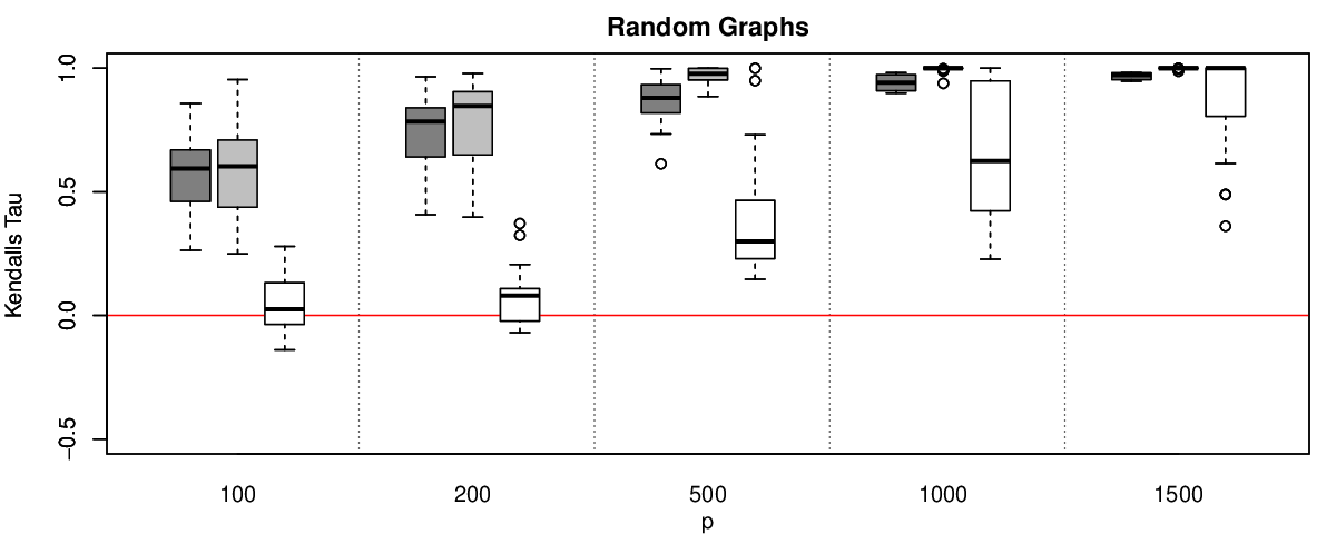
Refer to caption
Figure 6. Each boxplot represents 20 simulations with random DAGs when using a pre-selection step; in each case n=3/4​pn=3/4p. From left to right the methods are: the proposed high-dimensional LiNGAM procedure, same as Figure 5; the proposed high-dimensional LiNGAM procedure with pre-selection; the two stage pairwise procedure from Hyvärinen and Smith, (2013).

4.4. Data example: high-dimensional performance

We estimate causal structure among the stocks in the Standard and Poor’s 500. Specifically, we consider the percentage increase/decrease for each share price for each trading day between Jan 2007 to Sep 2017. We consider the p=442p=442 companies for which data is available for the entire period, and we scale and center the data so that each variable has mean 0 and variance 1. As structure may vary over time, we estimate the causal structure for each of the following periods separately with J=3J=3 and K=4K=4: 2007-2009, 2010-2011, 2012-2013, 2014-2015, 2016-2017 (ending in September). Across these periods, the sample size, nn, ranges from 425 to 755.

The underlying structure is unlikely to be causally sufficient or acyclic. In addition, although it is common to assume that daily returns are independent, this assumption may not hold in practice. Nonetheless, the method still recovers reasonable structure. We first consider the most recent Jan 2016 - Sep 2017 period. Figure 7 shows a boxplot for the estimated ordering of the companies within each sector. The sectors are sorted top to bottom by median ordering. Near the top, we see utilities, energy, real estate, and finance. Since energy is an input for almost every other sector, intuitively price movements in energy should be causally upstream of other sectors. The estimated ordering of utilities might seem surprising; however, utility stocks are typically thought of as a proxy for bond prices. Thus, the estimated ordering may reflect the fact that changes in utility stocks capture much of the causal effect of interest rates, which had stayed constant for much of 2011-2015 but began moving again in 2016. Real estate and finance, sectors that are highly impacted by interest rates, are also estimated to be early in the causal ordering.

Figure 8 ranks each sector by the median topological ordering for each period. The orderings are relatively stable over time, but there are a few notable changes. In 2007, real estate was estimated to be the “root sector” while finance is in the middle. This aligns with the idea that the root of the 2008 financial crisis was actually failing mortgage backed securities in real estate, which had a causal effect on finance. However, over time, real estate has moved more downstream.

5. Discussion

We proposed a causal discovery method that was proven consistent for specific test statistics and log concave errors. Similar analyses could be given for other statistics that are Lipschitz continuous in the sample moments over a bounded domain, can distinguish causal direction, and indicate the presence of confounding. This would include a normalized version of the proposed test statistics which accounts for the scaling of the data. Log-concavity was assumed for exponential concentration of sample moments and other distributional assumptions could be considered instead if analogous concentration results can be obtained and traced throughout the analysis.

The proposed algorithm requires selecting a bound on the in-degree JJ and a pruning parameter α\alpha. The in-degree is typically unknown, but a reasonable upper bound may be used as a “bet on sparsity”. If the maximum in-degree of the true graph is larger than the specified JJ but the “extra edges” have small enough edge-weights, the “closest” DAG with maximum in-degree JJ is still recovered with high probability. The pruning parameter α\alpha plays a similar role to the nominal level for each conditional independence test in the PC algorithm. Both parameters have an effect on the sparsity of the estimated graph and regulate the maximum size of conditioning sets.

Refer to caption
Figure 7. Estimated causal ordering of the stocks in the Standard and Poor’s 500 for Jan 2016 - Sep 2017. The stocks are grouped by sector, and the sectors are arranged by median causal ordering.
Refer to caption
Figure 8. Sectors ranked by median estimated topological ordering across each time period.

At each step, instead of taking the minimum |τ||\tau| over all subsets of potential parents, one could also pick parents for every unordered node using a variable selection procedure and then only calculate |τ||\tau| using the selected parents. Such a procedure would also consistently estimate the causal ordering as long as the variable selection procedure is consistent. Slightly different conditions, such as a beta-min condition, would be needed when adopting standard methods based on least squares, but in practice the resulting method performs quite well as shown in simulations in the supplement. This could be explained as being due to use of only second moments for the variable selection.

In (8), we have made a key restriction that the error moments must be adequately different from the moments of any Gaussian and the edge weights must be strongly parentally faithful. In practice, this is a difficult condition to satisfy, and Uhler et al., (2013) show that strong faithfulness type restrictions can be problematic in practice. However, even if the distribution is not strongly parentally faithful, we can still consistently recover the correct ordering as long as each individual linear coefficient is non-zero and the errors are sufficiently non-Gaussian. Sokol et al., (2014) consider identifiability of independent component analysis for fixed pp when the error terms are Gaussians contaminated with non-Gaussian noise. In particular, when the effect of the non-Gaussian contamination decreases at an adequately slow rate, the entire mixing matrix is identifiable asymptotically. In our analysis, the measure of non-Gaussianity is treated by our assumptions on γ\gamma. Our results suggest that the results of Sokol et al., (2014) can also be extended, given suitable sparsity, to the asymptotic regime where the number of variables is increasing.

The modified procedure we propose retains the existing benefits of the original DirectLiNGAM procedure. In particular, the output of algorithm is independent of the ordering of the variables in the input data. Although this is typically not an issue in the low-dimensional case, in the high-dimensional setting, the output of causal discovery methods may be highly dependent on ordering (Colombo and Maathuis,, 2014).

Acknowledgment

This work was supported by the U.S. National Science Foundation under Grant No. DMS 1712535. Thomas S. Richardson gave helpful feedback on an advance copy of the manuscript.

References

  • Colombo and Maathuis, (2014) Colombo, D. and Maathuis, M. H. (2014). Order-independent constraint-based causal structure learning. J. Mach. Learn. Res., 15:3741–3782.
  • Drton and Maathuis, (2017) Drton, M. and Maathuis, M. H. (2017). Structure learning in graphical modeling. Annual Review of Statistics and Its Application, 4(1):365–393.
  • Eddelbuettel and François, (2011) Eddelbuettel, D. and François, R. (2011). Rcpp: Seamless R and C++ integration. Journal of Statistical Software, 40(8):1–18.
  • Hao et al., (2012) Hao, D., Ren, C., and Li, C. (2012). Revisiting the variation of clustering coefficient of biological networks suggests new modular structure. BMC Systems Biology, 6(1):34.
  • Harris and Drton, (2013) Harris, N. and Drton, M. (2013). PC algorithm for nonparanormal graphical models. J. Mach. Learn. Res., 14:3365–3383.
  • Horn and Johnson, (2013) Horn, R. A. and Johnson, C. R. (2013). Matrix analysis. Cambridge University Press, Cambridge, second edition.
  • Hoyer et al., (2008) Hoyer, P. O., Hyvärinen, A., Scheines, R., Spirtes, P., Ramsey, J., Lacerda, G., and Shimizu, S. (2008). Causal discovery of linear acyclic models with arbitrary distributions. In UAI 2008, Proceedings of the 24th Conference in Uncertainty in Artificial Intelligence, Helsinki, Finland, July 9-12, 2008, pages 282–289.
  • Hyvärinen and Smith, (2013) Hyvärinen, A. and Smith, S. M. (2013). Pairwise likelihood ratios for estimation of non-Gaussian structural equation models. J. Mach. Learn. Res., 14:111–152.
  • Kalisch and Bühlmann, (2007) Kalisch, M. and Bühlmann, P. (2007). Estimating high-dimensional directed acyclic graphs with the pc-algorithm. J. Mach. Learn. Res., 8:613–636.
  • Lin et al., (2016) Lin, L., Drton, M., and Shojaie, A. (2016). Estimation of high-dimensional graphical models using regularized score matching. Electron. J. Stat., 10(1):806–854.
  • Loh and Bühlmann, (2014) Loh, P.-L. and Bühlmann, P. (2014). High-dimensional learning of linear causal networks via inverse covariance estimation. J. Mach. Learn. Res., 15:3065–3105.
  • Lumley, (2017) Lumley, T. (2017). leaps: Regression Subset Selection. R package version 3.0.
  • Maathuis et al., (2009) Maathuis, M. H., Kalisch, M., and Bühlmann, P. (2009). Estimating high-dimensional intervention effects from observational data. Ann. Statist., 37(6A):3133–3164.
  • Meinshausen and Bühlmann, (2006) Meinshausen, N. and Bühlmann, P. (2006). High-dimensional graphs and variable selection with the lasso. Ann. Statist., 34(3):1436–1462.
  • Okamoto, (1973) Okamoto, M. (1973). Distinctness of the eigenvalues of a quadratic form in a multivariate sample. Ann. Statist., 1:763–765.
  • Pearl, (2009) Pearl, J. (2009). Causality. Cambridge University Press, Cambridge, second edition. Models, reasoning, and inference.
  • Peters and Bühlmann, (2014) Peters, J. and Bühlmann, P. (2014). Identifiability of Gaussian structural equation models with equal error variances. Biometrika, 101(1):219–228.
  • R Core Team, (2017) R Core Team (2017). R: a language and environment for statistical computing. R Foundation for Statistical Computing, Vienna, Austria.
  • Rothenhäusler et al., (2018) Rothenhäusler, D., Ernest, J., and Bühlmann, P. (2018). Causal inference in partially linear structural equation models. Ann. Statist., 46(6A):2904–2938.
  • Shimizu et al., (2006) Shimizu, S., Hoyer, P. O., Hyvärinen, A., and Kerminen, A. (2006). A linear non-Gaussian acyclic model for causal discovery. J. Mach. Learn. Res., 7:2003–2030.
  • Shimizu et al., (2011) Shimizu, S., Inazumi, T., Sogawa, Y., Hyvärinen, A., Kawahara, Y., Washio, T., Hoyer, P. O., and Bollen, K. (2011). DirectLiNGAM: a direct method for learning a linear non-Gaussian structural equation model. J. Mach. Learn. Res., 12:1225–1248.
  • Sokol et al., (2014) Sokol, A., Maathuis, M. H., and Falkeborg, B. (2014). Quantifying identifiability in independent component analysis. Electron. J. Stat., 8(1):1438–1459.
  • Spirtes et al., (2000) Spirtes, P., Glymour, C., and Scheines, R. (2000). Causation, prediction, and search. Adaptive Computation and Machine Learning. MIT Press, Cambridge, MA, second edition. With additional material by David Heckerman, Christopher Meek, Gregory F. Cooper and Thomas Richardson, A Bradford Book.
  • Steinsky, (2013) Steinsky, B. (2013). Enumeration of labelled essential graphs. Ars Combin., 111:485–494.
  • Uhler et al., (2013) Uhler, C., Raskutti, G., Bühlmann, P., and Yu, B. (2013). Geometry of the faithfulness assumption in causal inference. Ann. Statist., 41(2):436–463.

Appendix A Proof of Theorem 1

Proof.

Statement (i): Consider any set CC such that pa⁡(v)⊆C{\rm pa}(v)\subseteq C and C∩de⁡(v)=∅C\cap{\rm de}(v)=\emptyset. Since we condition on all parents, βv​c.C=0\beta_{vc.C}=0 for any c∈Cc\in C which is not a parent of vv. Then,

(13) Yv.C\displaystyle Y_{v.C} =Yv−∑c∈pa⁡(v)βv​c.C​Yc−∑k∈C∖pa⁡(v)βv​c.C​Yc\displaystyle=Y_{v}-\sum_{c\in{\rm pa}(v)}\beta_{vc.C}Y_{c}-\sum_{k\in C\setminus{\rm pa}(v)}\beta_{vc.C}Y_{c}
=Yv−∑c∈pa⁡(v)βv​c.C​Yc\displaystyle=Y_{v}-\sum_{c\in{\rm pa}(v)}\beta_{vc.C}Y_{c}
=εv.\displaystyle=\varepsilon_{v}.

We then directly calculate the parameter for the set CC:

(14) τv.C→u(K)\displaystyle\tau^{(K)}_{v.C\rightarrow u} =𝔼⁡(Yv.CK−1​Yu)​𝔼​(Yv.C2)−𝔼⁡(Yv.CK)​𝔼​(Yv.C​Yu)\displaystyle={\mathbb{E}}(Y_{v.C}^{K-1}Y_{u}){\mathbb{E}}(Y_{v.C}^{2})-{\mathbb{E}}(Y_{v.C}^{K}){\mathbb{E}}(Y_{v.C}Y_{u})
=𝔼⁡{εvK−1​(εu+πu​v​εv+∑z∈an⁡(u)∖{v}πu​z​εz)}​𝔼​(εv2)\displaystyle=\textstyle{\mathbb{E}}\left\{\varepsilon_{v}^{K-1}\left(\varepsilon_{u}+\pi_{uv}\varepsilon_{v}+\sum_{z\in{\rm an}(u)\setminus\{v\}}\pi_{uz}\varepsilon_{z}\right)\right\}{\mathbb{E}}\left(\varepsilon_{v}^{2}\right)
−𝔼⁡(εvK)​𝔼​{εv​(εu+πu​v​εv+∑z∈an⁡(u)∖{v}πu​z​εz)}\displaystyle\textstyle\quad-{\mathbb{E}}\left(\varepsilon_{v}^{K}\right){\mathbb{E}}\left\{\varepsilon_{v}\left(\varepsilon_{u}+\pi_{uv}\varepsilon_{v}+\sum_{z\in{\rm an}(u)\setminus\{v\}}\pi_{uz}\varepsilon_{z}\right)\right\}
=πu​v​𝔼​(εvK)​𝔼​(εv2)−πu​v​𝔼​(εvK)​𝔼​(εv2)\displaystyle=\pi_{uv}{\mathbb{E}}\left(\varepsilon_{v}^{K}\right){\mathbb{E}}\left(\varepsilon_{v}^{2}\right)-\pi_{uv}{\mathbb{E}}\left(\varepsilon_{v}^{K}\right){\mathbb{E}}\left(\varepsilon_{v}^{2}\right)
=0.\displaystyle=0.

The penultimate equality follows from the assumption of independent errors.∎

Statement (ii): For fixed CC, u,v∈Vu,v\in V, and parentally faithful linear coefficients and variances, τv.C→u(K)\tau^{(K)}_{v.C\rightarrow u} is a polynomial of the error moments of degree k=3,…,Kk=3,\ldots,K. Thus, selecting a single point (of error moments) where the quantity τv.C→u\tau_{v.C\rightarrow u} is non-zero is sufficient for showing that the quantity is non-zero for generic error moments of degree k=3,…,Kk=3,\ldots,K (Okamoto,, 1973). Specifically, we select that point by letting all error moments for k<Kk<K be consistent with the Gaussian moments implied by σv2\sigma_{v}^{2}, the variance of εv\varepsilon_{v}, but select the KKth degree moment to be inconsistent with the corresponding Gaussian moment. Since there are a finite number of sets C⊆VC\subseteq V such that C∩de⁡(v)=∅C\cap{\rm de}(v)=\emptyset, then the set of error moments of degree k=3,…,Kk=3,\ldots,K which yield τv.C→u=0\tau_{v.C\rightarrow u}=0 for any C⊆VC\subseteq V also has Lebesgue measure zero.

Recall that the total residual effect of uu on vv given CC is

πv​u.C=πv​u−∑c∈Cβv​c.C​πc​u,\pi_{vu.C}=\pi_{vu}-\sum_{c\in C}\beta_{vc.C}\pi_{cu},

where πv​u\pi_{vu} is the total effect of uu on vv and πu​u=1\pi_{uu}=1. Now,

(15) Yv.C\displaystyle Y_{v.C} =Yv−∑c∈Cβv​c.C​Yc\displaystyle=Y_{v}-\sum_{c\in C}\beta_{vc.C}Y_{c}
=εv+∑k∈an⁡(v)πv​k​εk−∑c∈Cβv​c.C​∑d∈An⁡(c)πc​d​εd\displaystyle=\varepsilon_{v}+\sum_{k\in{\rm an}(v)}\pi_{vk}\varepsilon_{k}-\sum_{c\in C}\beta_{vc.C}\sum_{d\in{\rm An}(c)}\pi_{cd}\varepsilon_{d}
=εv+∑k∈an⁡(v)∪An⁡(C)πv​k.C​εk.\displaystyle=\varepsilon_{v}+\sum_{k\in{\rm an}(v)\cup{\rm An}(C)}\pi_{vk.C}\varepsilon_{k}.

By the parental faithfulness assumption, since u∈pa⁡(v)u\in{\rm pa}(v), πv​u.C≠0\pi_{vu.C}\neq 0. We partition An⁡(v)∪An⁡(C){\rm An}(v)\cup{\rm An}(C) into three disjoint sets

(16) Z1\displaystyle Z_{1} ={An⁡(v)∪An⁡(C)}∖An⁡(u),\displaystyle=\left\{{\rm An}(v)\cup{\rm An}(C)\right\}\setminus{\rm An}(u),
Z2\displaystyle Z_{2} ={z∈An⁡(u):πv​z.C=πv​u.C​πu​z}, and\displaystyle=\{z\in{\rm An}(u):\pi_{vz.C}=\pi_{vu.C}\pi_{uz}\},\text{ and }
Z3\displaystyle Z_{3} =An⁡(u)∖Z2.\displaystyle={\rm An}(u)\setminus Z_{2}.

For generic edge weights, Z2∖{u}Z_{2}\setminus\{u\} corresponds to ancestors of uu which only have directed paths to vv through C∪{u}C\cup\{u\}; Z3Z_{3} corresponds to ancestors of uu which have directed paths to vv that do not pass through C∪{u}C\cup\{u\}. For some specific edge weight values, Z2Z_{2} may also include non ancestors of uu which have directed paths to vv that do not pass through C∪{u}C\cup\{u\} if those paths do not contribute to the total effect; i.e., non-faithfulness may result in Z2Z_{2} including more nodes. However, Z2Z_{2} is non-empty because u∈Z2u\in Z_{2} by the parental faithfulness assumption.

Let

εZ1\displaystyle\varepsilon_{Z_{1}} =εv+∑z∈Z1πv​z.C​εz,\displaystyle=\varepsilon_{v}+\sum_{z\in Z_{1}}\pi_{vz.C}\varepsilon_{z},
εZ2\displaystyle\varepsilon_{Z_{2}} =∑z∈Z2πu​z​εz,\displaystyle=\sum_{z\in Z_{2}}\pi_{uz}\varepsilon_{z},
εZ3\displaystyle\varepsilon_{Z_{3}} =∑z∈Z3(πv​z−∑c∈Cβv​c.C​πc​z)​εz=∑z∈Z3πv​z.C​εz,\displaystyle=\sum_{z\in Z_{3}}\bigg(\pi_{vz}-\sum_{c\in C}\beta_{vc.C}\pi_{cz}\bigg)\varepsilon_{z}=\sum_{z\in Z_{3}}\pi_{vz.C}\varepsilon_{z},

so that

Yv.C=εZ1+πv​u.C​εZ2+εZ3Y_{v.C}=\varepsilon_{Z_{1}}+\pi_{vu.C}\varepsilon_{Z_{2}}+\varepsilon_{Z_{3}}

and

Yu=εZ2+∑z∈Z3πu​z​εz.Y_{u}=\varepsilon_{Z_{2}}+\sum_{z\in Z_{3}}\pi_{uz}\varepsilon_{z}.

For w=(w1,w2,w3)w=(w_{1},w_{2},w_{3}) with |w|=w0|w|=w_{0}, let (w0w)=w0!w1!​w2!​w3!\binom{w_{0}}{w}=\frac{w_{0}!}{w_{1}!w_{2}!w_{3}!}, the multinomial coefficient. Then

(17) Yv.Cw0\displaystyle Y_{v.C}^{w_{0}} =(εZ1+πv​u.C​εZ2+εZ3)w0=∑|w|=w0(w0w)​εZ1w1​(πv​u.C​εZ2)w2​εZ3w3\displaystyle=\left(\varepsilon_{Z_{1}}+\pi_{vu.C}\varepsilon_{Z_{2}}+\varepsilon_{Z_{3}}\right)^{w_{0}}=\sum_{|w|=w_{0}}\binom{w_{0}}{w}\varepsilon_{Z_{1}}^{w_{1}}(\pi_{vu.C}\varepsilon_{Z_{2}})^{w_{2}}\varepsilon_{Z_{3}}^{w_{3}}
=∑|w|=w0w3=0(w0w)​εZ1w1​(πv​u.C​εZ2)w2​εZ3w3+∑|w|=w0w3>0(w0w)​εZ1w1​(πv​u.C​εZ2)w2​εZ3w3\displaystyle=\sum_{\begin{subarray}{c}|w|=w_{0}\\ w_{3}=0\end{subarray}}{w_{0}\choose w}\varepsilon_{Z_{1}}^{w_{1}}(\pi_{vu.C}\varepsilon_{Z_{2}})^{w_{2}}\varepsilon_{Z_{3}}^{w_{3}}+\sum_{\begin{subarray}{c}|w|=w_{0}\\ w_{3}>0\end{subarray}}{w_{0}\choose w}\varepsilon_{Z_{1}}^{w_{1}}(\pi_{vu.C}\varepsilon_{Z_{2}})^{w_{2}}\varepsilon_{Z_{3}}^{w_{3}}
=(εZ1+πv​u.C​εZ2)w0+∑|w|=w0w3>0(w0w)​εZ1w1​(πv​u.C​εZ2)w2​εZ3w3,\displaystyle=(\varepsilon_{Z_{1}}+\pi_{vu.C}\varepsilon_{Z_{2}})^{w_{0}}+\sum_{\begin{subarray}{c}|w|=w_{0}\\ w_{3}>0\end{subarray}}\binom{w_{0}}{w}\varepsilon_{Z_{1}}^{w_{1}}(\pi_{vu.C}\varepsilon_{Z_{2}})^{w_{2}}\varepsilon_{Z_{3}}^{w_{3}},

so that

(18) τv.C→u(K)\displaystyle\tau^{(K)}_{v.C\rightarrow u} =𝔼⁡(Yv.CK−1​Yu)​𝔼​(Yv.C2)−𝔼⁡(Yv.CK)​𝔼​(Yv.C​Yu)\displaystyle={\mathbb{E}}(Y_{v.C}^{K-1}Y_{u}){\mathbb{E}}(Y_{v.C}^{2})-{\mathbb{E}}(Y_{v.C}^{K}){\mathbb{E}}(Y_{v.C}Y_{u})
=𝔼⁡{(εZ1+πv​u.C​εZ2+εZ3)K−1​Yu}​𝔼​{(εZ1+πv​u.C​εZ2+εZ3)2}\displaystyle={\mathbb{E}}\left\{\left(\varepsilon_{Z_{1}}+\pi_{vu.C}\varepsilon_{Z_{2}}+\varepsilon_{Z_{3}}\right)^{K-1}Y_{u}\right\}{\mathbb{E}}\left\{\left(\varepsilon_{Z_{1}}+\pi_{vu.C}\varepsilon_{Z_{2}}+\varepsilon_{Z_{3}}\right)^{2}\right\}
−𝔼⁡{(εZ1+πv​u.C​εZ2+εZ3)K}​𝔼​{(εZ1+πv​u.C​εZ2+εZ3)​Yu}\displaystyle\quad-{\mathbb{E}}\left\{\left(\varepsilon_{Z_{1}}+\pi_{vu.C}\varepsilon_{Z_{2}}+\varepsilon_{Z_{3}}\right)^{K}\right\}{\mathbb{E}}\left\{\left(\varepsilon_{Z_{1}}+\pi_{vu.C}\varepsilon_{Z_{2}}+\varepsilon_{Z_{3}}\right)Y_{u}\right\}
=(σZ12+πv​u.C2σZ22+σZ32)[𝔼{(εZ1+πv​u.CεZ2)K−1Yu}\displaystyle=\left(\sigma_{Z_{1}}^{2}+\pi_{vu.C}^{2}\sigma_{Z_{2}}^{2}+\sigma_{Z_{3}}^{2}\right)\left[{\mathbb{E}}\left\{(\varepsilon_{Z_{1}}+\pi_{vu.C}\varepsilon_{Z_{2}})^{K-1}Y_{u}\right\}\vphantom{{\mathbb{E}}\left\{Y_{u}\sum_{\begin{subarray}{c}|w|=K-1\\ w_{3}>0\end{subarray}}\binom{K-1}{w}\varepsilon_{Z_{1}}^{w_{1}}(\pi_{vu.C}\varepsilon_{Z_{2}})^{w_{2}}\varepsilon_{Z_{3}}^{w_{3}}\right\}}\right.
+𝔼{Yu∑|w|=K−1w3>0(K−1w)εZ1w1(πv​u.CεZ2)w2εZ3w3}]\displaystyle\left.\hphantom{\left(\sigma_{Z_{1}}^{2}+\pi_{vu.C}^{2}\sigma_{Z_{2}}^{2}+\sigma_{Z_{3}}^{2}\right)}\quad\quad+{\mathbb{E}}\left\{Y_{u}\sum_{\begin{subarray}{c}|w|=K-1\\ w_{3}>0\end{subarray}}\binom{K-1}{w}\varepsilon_{Z_{1}}^{w_{1}}(\pi_{vu.C}\varepsilon_{Z_{2}})^{w_{2}}\varepsilon_{Z_{3}}^{w_{3}}\right\}\right]
−[𝔼⁡{(εZ1+πv​u.C​εZ2)K}+𝔼⁡{∑|w|=Kw3>0(Kw)​εZ1w1​(πv​u.C​εZ2)w2​εZ3w3}]\displaystyle\quad-\left[{\mathbb{E}}\left\{(\varepsilon_{Z_{1}}+\pi_{vu.C}\varepsilon_{Z_{2}})^{K}\right\}+{\mathbb{E}}\left\{\sum_{\begin{subarray}{c}|w|=K\\ w_{3}>0\end{subarray}}{K\choose w}\varepsilon_{Z_{1}}^{w_{1}}(\pi_{vu.C}\varepsilon_{Z_{2}})^{w_{2}}\varepsilon_{Z_{3}}^{w_{3}}\right\}\right]
×{πv​u.C​σZ22+𝔼⁡(εZ3​Yu)}.\displaystyle\quad\times\left\{\pi_{vu.C}\sigma_{Z_{2}}^{2}+{\mathbb{E}}\left(\varepsilon_{Z_{3}}Y_{u}\right)\right\}.

We first consider the case where Z3Z_{3} is empty so that the expansion above reduces to

(19) τv.C→u(K)\displaystyle\tau^{(K)}_{v.C\rightarrow u} =[𝔼⁡{(εZ1+πv​u.C​εZ2)K−1​Yu}]×(σZ12+πv​u.C2​σZ22)\displaystyle=\left[{\mathbb{E}}\left\{(\varepsilon_{Z_{1}}+\pi_{vu.C}\varepsilon_{Z_{2}})^{K-1}Y_{u}\right\}\right]\times\left(\sigma_{Z_{1}}^{2}+\pi_{vu.C}^{2}\sigma_{Z_{2}}^{2}\right)
−[𝔼{(εZ1+πv​u.CεZ2)k}]×(πv​u.CσZ22).\displaystyle\quad-\left[{\mathbb{E}}\left\{(\varepsilon_{Z_{1}}+\pi_{vu.C}\varepsilon_{Z_{2}})^{k}\right\}\right]\times\left(\pi_{vu.C}\sigma_{Z_{2}}^{2}\right).

Let the moments of degree kk for 2<k<K2<k<K of all the error terms be consistent with some Gaussian distribution. This implies that the error moments for z=Z1,Z2z=Z_{1},Z_{2} are also consistent with some Gaussian distribution since the sum of Gaussians is also Gaussian. So 𝔼⁡(εz2)=σz2{\mathbb{E}}(\varepsilon_{z}^{2})=\sigma_{z}^{2} and for k<Kk<K,

E⁡(εzk)={0 if ​k​ is odd,(k−1)!!​σzk if ​k​ is even,E(\varepsilon_{z}^{k})=\begin{cases}0&\text{ if }k\text{ is odd},\\ (k-1)!!\sigma_{z}^{k}&\text{ if }k\text{ is even},\end{cases}

where k!!k!! is the double factorial of kk. However, let the KKth degree error moments be inconsistent with the specified Gaussian distribution so that for z=Z1,Z2z=Z_{1},Z_{2} and ηz>0\eta_{z}>0,

E⁡(εzK)={ηz if ​K​ is odd,(K−1)!!​σzK+ηz if ​K​ is even.E(\varepsilon_{z}^{K})=\begin{cases}\eta_{z}&\text{ if }K\text{ is odd},\\ (K-1)!!\sigma_{z}^{K}+\eta_{z}&\text{ if }K\text{ is even.}\\ \end{cases}

By direct calculation we see

τv.C→u(K)\displaystyle\tau^{(K)}_{v.C\rightarrow u} =𝔼⁡(Yv.CK−1​Yu)​𝔼​(Yv.C2)−𝔼⁡(Yv.CK)​𝔼​(Yv.C​Yu)\displaystyle={\mathbb{E}}(Y_{v.C}^{K-1}Y_{u}){\mathbb{E}}(Y_{v.C}^{2})-{\mathbb{E}}(Y_{v.C}^{K}){\mathbb{E}}(Y_{v.C}Y_{u})
=𝔼⁡{(εZ1+πv​u.C​εZ2)K−1​Yu}​𝔼​{(εZ1+πv​u.C​εZ2)2}\displaystyle={\mathbb{E}}\left\{(\varepsilon_{Z_{1}}+\pi_{vu.C}\varepsilon_{Z_{2}})^{K-1}Y_{u}\right\}{\mathbb{E}}\left\{(\varepsilon_{Z_{1}}+\pi_{vu.C}\varepsilon_{Z_{2}})^{2}\right\}
−𝔼⁡{(εZ1+πv​u.C​εZ2)K}​𝔼​{(εZ1+πv​u.C​εZ2)​(Yu)}\displaystyle\qquad-{\mathbb{E}}\left\{(\varepsilon_{Z_{1}}+\pi_{vu.C}\varepsilon_{Z_{2}})^{K}\right\}{\mathbb{E}}\left\{(\varepsilon_{Z_{1}}+\pi_{vu.C}\varepsilon_{Z_{2}})(Y_{u})\right\}
={∑a=0K−1(K−1a)​𝔼​(εZ1a)​𝔼​(πv​u.CK−1−a​εZ2K−1−a​Yu)}​{𝔼⁡(εZ12)+𝔼⁡(πv​u.C2​εZ22)}\displaystyle=\textstyle\left\{\sum_{a=0}^{K-1}{K-1\choose a}{\mathbb{E}}\left(\varepsilon_{Z_{1}}^{a}\right){\mathbb{E}}\left(\pi_{vu.C}^{K-1-a}\varepsilon_{Z_{2}}^{K-1-a}Y_{u}\right)\right\}\left\{{\mathbb{E}}(\varepsilon_{Z_{1}}^{2})+{\mathbb{E}}(\pi_{vu.C}^{2}\varepsilon_{Z_{2}}^{2})\right\}
−{∑a=0K(Ka)​𝔼​(εZ1a)​𝔼​(πv​u.CK−a​εZ2K−a​Yu)}​𝔼​(πv​u.C​εZ2​Yu)\displaystyle\textstyle\qquad-\left\{\sum_{a=0}^{K}{K\choose a}{\mathbb{E}}\left(\varepsilon_{Z_{1}}^{a}\right){\mathbb{E}}\left(\pi_{vu.C}^{K-a}\varepsilon_{Z_{2}}^{K-a}Y_{u}\right)\right\}{\mathbb{E}}\left(\pi_{vu.C}\varepsilon_{Z_{2}}Y_{u}\right)
={∑a=1K−1(K−1a)​𝔼​(εZ1a)​πv​u.CK−1−a​𝔼​(εZ2K−a)}​{𝔼⁡(εZ12)+πv​u.C2​𝔼​(εZ22)}\displaystyle\textstyle=\left\{\sum_{a=1}^{K-1}{K-1\choose a}{\mathbb{E}}\left(\varepsilon_{Z_{1}}^{a}\right)\pi_{vu.C}^{K-1-a}{\mathbb{E}}\left(\varepsilon_{Z_{2}}^{K-a}\right)\right\}\left\{{\mathbb{E}}(\varepsilon_{Z_{1}}^{2})+\pi_{vu.C}^{2}{\mathbb{E}}(\varepsilon_{Z_{2}}^{2})\right\}
−{∑a=1K−1(Ka)​𝔼​(εZ1a)​πv​u.CK−a​𝔼​(εZ2K−a)}​πv​u.C​𝔼​(εZ22)\displaystyle\textstyle\qquad-\left\{\sum_{a=1}^{K-1}{K\choose a}{\mathbb{E}}\left(\varepsilon_{Z_{1}}^{a}\right)\pi_{vu.C}^{K-a}{\mathbb{E}}\left(\varepsilon_{Z_{2}}^{K-a}\right)\right\}\pi_{vu.C}{\mathbb{E}}\left(\varepsilon_{Z_{2}}^{2}\right)
+πv​u.CK−1​𝔼​(εZ2K)​{𝔼⁡(εZ12)+πv​u.C2​𝔼​(εZ22)}\displaystyle\textstyle\qquad+\pi_{vu.C}^{K-1}{\mathbb{E}}(\varepsilon_{Z_{2}}^{K})\left\{{\mathbb{E}}(\varepsilon_{Z_{1}}^{2})+\pi_{vu.C}^{2}{\mathbb{E}}(\varepsilon_{Z_{2}}^{2})\right\}
−{πv​u.CK​𝔼​(εZ2K)+𝔼⁡(εZ1K)}​πv​u.C​𝔼​(εZ22)\displaystyle\textstyle\qquad-\left\{\pi_{vu.C}^{K}{\mathbb{E}}(\varepsilon_{Z_{2}}^{K})+{\mathbb{E}}(\varepsilon_{Z_{1}}^{K})\right\}\pi_{vu.C}{\mathbb{E}}(\varepsilon_{Z_{2}}^{2})
={∑a=1K−1(K−1a)​πv​u.CK−1−a​𝔼​(εZ1a)​𝔼​(εZ2K−a)}​{𝔼⁡(εZ12)+πv​u.C2​𝔼​(εZ22)}\displaystyle\textstyle=\left\{\sum_{a=1}^{K-1}{K-1\choose a}\pi_{vu.C}^{K-1-a}{\mathbb{E}}\left(\varepsilon_{Z_{1}}^{a}\right){\mathbb{E}}\left(\varepsilon_{Z_{2}}^{K-a}\right)\right\}\left\{{\mathbb{E}}(\varepsilon_{Z_{1}}^{2})+\pi_{vu.C}^{2}{\mathbb{E}}(\varepsilon_{Z_{2}}^{2})\right\}
−{∑a=1K−1(Ka)​𝔼​(εZ1a)​πv​u.CK−a​𝔼​(εZ2K−a)}​πv​u.C​𝔼​(εZ22)\displaystyle\textstyle\qquad-\left\{\sum_{a=1}^{K-1}{K\choose a}{\mathbb{E}}\left(\varepsilon_{Z_{1}}^{a}\right)\pi_{vu.C}^{K-a}{\mathbb{E}}\left(\varepsilon_{Z_{2}}^{K-a}\right)\right\}\pi_{vu.C}{\mathbb{E}}\left(\varepsilon_{Z_{2}}^{2}\right)
+πv​u.CK−1​𝔼​(εZ2K)​𝔼​(εZ12)−πv​u.C​𝔼​(εZ1K)​𝔼​(εZ22).\displaystyle\textstyle\qquad+\pi_{vu.C}^{K-1}{\mathbb{E}}(\varepsilon_{Z_{2}}^{K}){\mathbb{E}}(\varepsilon_{Z_{1}}^{2})-\pi_{vu.C}{\mathbb{E}}(\varepsilon_{Z_{1}}^{K}){\mathbb{E}}(\varepsilon_{Z_{2}}^{2}).

When KK is odd, 𝔼⁡(εZ1a)​𝔼​(εZ2K−a)=0{\mathbb{E}}(\varepsilon_{Z_{1}}^{a}){\mathbb{E}}(\varepsilon_{Z_{2}}^{K-a})=0 for all a=1,…,K−1a=1,\ldots,K-1, so we are left with

(20) τv.C→u(K)\displaystyle\tau^{(K)}_{v.C\rightarrow u} =πv​u.CK−1​𝔼​(εZ2K)​σZ12−πv​u.C​𝔼​(εZ1K)​σZ22\displaystyle=\pi_{vu.C}^{K-1}{\mathbb{E}}(\varepsilon_{Z_{2}}^{K})\sigma_{Z_{1}}^{2}-\pi_{vu.C}{\mathbb{E}}(\varepsilon_{Z_{1}}^{K})\sigma_{Z_{2}}^{2}
=πv​u.CK−1​ηZ2​σZ12−πv​u.C​ηZ1​σZ22.\displaystyle=\pi_{vu.C}^{K-1}\eta_{Z_{2}}\sigma_{Z_{1}}^{2}-\pi_{vu.C}\eta_{Z_{1}}\sigma_{Z_{2}}^{2}.

When KK is even, then 𝔼⁡(εZ1a)​𝔼​(YuK−a)=0{\mathbb{E}}(\varepsilon_{Z_{1}}^{a}){\mathbb{E}}(Y_{u}^{K-a})=0 when aa is odd, so we are left with

τv.C→u(K)\displaystyle\tau^{(K)}_{v.C\rightarrow u} ={∑a=2,4,…,K−2(K−1a)​πv​u.CK−1−a​𝔼​(εZ1a)​𝔼​(εZ2K−a)}​{𝔼⁡(εZ12)+πv​u.C2​𝔼​(εZ22)}\displaystyle=\textstyle\left\{\sum_{a=2,4,\ldots,K-2}{K-1\choose a}\pi_{vu.C}^{K-1-a}{\mathbb{E}}\left(\varepsilon_{Z_{1}}^{a}\right){\mathbb{E}}\left(\varepsilon_{Z_{2}}^{K-a}\right)\right\}\left\{{\mathbb{E}}(\varepsilon_{Z_{1}}^{2})+\pi_{vu.C}^{2}{\mathbb{E}}(\varepsilon_{Z_{2}}^{2})\right\}
−{∑a=2,4,…,K−2(Ka)​𝔼​(εZ1a)​πv​u.CK−a​𝔼​(εZ2K−a)}​πv​u.C​𝔼​(εZ22)\displaystyle\textstyle\qquad-\left\{\sum_{a=2,4,\ldots,K-2}{K\choose a}{\mathbb{E}}\left(\varepsilon_{Z_{1}}^{a}\right)\pi_{vu.C}^{K-a}{\mathbb{E}}\left(\varepsilon_{Z_{2}}^{K-a}\right)\right\}\pi_{vu.C}{\mathbb{E}}\left(\varepsilon_{Z_{2}}^{2}\right)
+πv​u.CK−1​𝔼​(εZ2K)​𝔼​(εZ12)−πv​u.C​𝔼​(εZ1K)​𝔼​(εZ22).\displaystyle\textstyle\qquad+\pi_{vu.C}^{K-1}{\mathbb{E}}(\varepsilon_{Z_{2}}^{K}){\mathbb{E}}(\varepsilon_{Z_{1}}^{2})-\pi_{vu.C}{\mathbb{E}}(\varepsilon_{Z_{1}}^{K}){\mathbb{E}}(\varepsilon_{Z_{2}}^{2}).

Evaluating the moments yields

τv.C→u(K)\displaystyle\tau^{(K)}_{v.C\rightarrow u} ={∑a=2,…,K−2(K−1a)​πv​u.CK−1−a​(a−1)!!​σZ1a​(K−a−1)!!​σZ2K−a}​(σZ12+πv​u.C2​σZ22)\displaystyle=\textstyle\left\{\sum_{a=2,\ldots,K-2}{K-1\choose a}\pi_{vu.C}^{K-1-a}(a-1)!!\sigma_{Z_{1}}^{a}(K-a-1)!!\sigma_{Z_{2}}^{K-a}\right\}\left(\sigma_{Z_{1}}^{2}+\pi_{vu.C}^{2}\sigma_{Z_{2}}^{2}\right)
−{∑a=2,…,K−2(Ka)⁡(a−1)!!​σZ1a​πv​u.CK−a​(K−a−1)!!​σZ2K−a}​(πv​u.C​σZ22)\displaystyle\textstyle\qquad-\left\{\sum_{a=2,\ldots,K-2}{K\choose a}(a-1)!!\sigma_{Z_{1}}^{a}\pi_{vu.C}^{K-a}(K-a-1)!!\sigma_{Z_{2}}^{K-a}\right\}\left(\pi_{vu.C}\sigma_{Z_{2}}^{2}\right)
+πv​u.CK−1​𝔼​(εZ2K)​σZ12−πv​u.C​𝔼​(εZ1K)​σZ22\displaystyle\textstyle\qquad+\pi_{vu.C}^{K-1}{\mathbb{E}}(\varepsilon_{Z_{2}}^{K})\sigma_{Z_{1}}^{2}-\pi_{vu.C}{\mathbb{E}}(\varepsilon_{Z_{1}}^{K})\sigma_{Z_{2}}^{2}
={∑a=2,…,K−2(K−1a)​πv​u.CK−1−a​(a−1)!!​σZ1a+2​(K−a−1)!!​σZ2K−a}\displaystyle\textstyle=\left\{\sum_{a=2,\ldots,K-2}{K-1\choose a}\pi_{vu.C}^{K-1-a}(a-1)!!\sigma_{Z_{1}}^{a+2}(K-a-1)!!\sigma_{Z_{2}}^{K-a}\right\}
+πv​u.C​σZ22​{∑a=2,…,K−2(K−1a)​πv​u.CK−a​(a−1)!!​σZ1a​(K−a−1)!!​σZ2K−a}\displaystyle\textstyle\qquad+\pi_{vu.C}\sigma_{Z_{2}}^{2}\left\{\sum_{a=2,\ldots,K-2}{K-1\choose a}\pi_{vu.C}^{K-a}(a-1)!!\sigma_{Z_{1}}^{a}(K-a-1)!!\sigma_{Z_{2}}^{K-a}\right\}
−{∑a=2,…,K−2(K−1a)​KK−a​(a−1)!!​σZ1a​πv​u.CK−a​(K−a−1)!!​σZ2K−a}​(πv​u.C​σZ22)\displaystyle\textstyle\qquad-\left\{\sum_{a=2,\ldots,K-2}{K-1\choose a}\frac{K}{K-a}(a-1)!!\sigma_{Z_{1}}^{a}\pi_{vu.C}^{K-a}(K-a-1)!!\sigma_{Z_{2}}^{K-a}\right\}\left(\pi_{vu.C}\sigma_{Z_{2}}^{2}\right)
+πv​u.CK−1​𝔼​(εZ2K)​σZ12−πv​u.C​𝔼​(εZ1K)​σZ22\displaystyle\textstyle\qquad+\pi_{vu.C}^{K-1}{\mathbb{E}}(\varepsilon_{Z_{2}}^{K})\sigma_{Z_{1}}^{2}-\pi_{vu.C}{\mathbb{E}}(\varepsilon_{Z_{1}}^{K})\sigma_{Z_{2}}^{2}
={∑a=2,…,K−2(K−1a)​πv​u.CK−1−a​(a−1)!!​σZ1a+2​(K−a−1)!!​σZ2K−a}\displaystyle\textstyle=\left\{\sum_{a=2,\ldots,K-2}{K-1\choose a}\pi_{vu.C}^{K-1-a}(a-1)!!\sigma_{Z_{1}}^{a+2}(K-a-1)!!\sigma_{Z_{2}}^{K-a}\right\}
+{∑a=2,…,K−2(K−1a)⁡(1−KK−a)​(a−1)!!​σZ1a​πv​u.CK−a​(K−a−1)!!​σZ2K−a}\displaystyle\textstyle\qquad+\left\{\sum_{a=2,\ldots,K-2}{K-1\choose a}\left(1-\frac{K}{K-a}\right)(a-1)!!\sigma_{Z_{1}}^{a}\pi_{vu.C}^{K-a}(K-a-1)!!\sigma_{Z_{2}}^{K-a}\right\}
×(πv​u.C​σZ22)\displaystyle\textstyle\qquad\times\left(\pi_{vu.C}\sigma_{Z_{2}}^{2}\right)
+πv​u.CK−1​𝔼​(εZ2K)​σZ12−πv​u.C​𝔼​(εZ1K)​σZ22\displaystyle\textstyle\qquad+\pi_{vu.C}^{K-1}{\mathbb{E}}(\varepsilon_{Z_{2}}^{K})\sigma_{Z_{1}}^{2}-\pi_{vu.C}{\mathbb{E}}(\varepsilon_{Z_{1}}^{K})\sigma_{Z_{2}}^{2}
={∑a=2,…,K−4(K−1a)​πv​u.CK−1−a​(a−1)!!​σZ1a+2​(K−a−1)!!​σZ2K−a}\displaystyle\textstyle=\left\{\sum_{a=2,\ldots,K-4}{K-1\choose a}\pi_{vu.C}^{K-1-a}(a-1)!!\sigma_{Z_{1}}^{a+2}(K-a-1)!!\sigma_{Z_{2}}^{K-a}\right\}
−{∑a=4,…,K−2(K−1a)​aK−a​(a−1)!!​σZ1a​πv​u.CK−a​(K−a−1)!!​σZ2K−a}​(πv​u.C​σZ22)\displaystyle\textstyle\qquad-\left\{\sum_{a=4,\ldots,K-2}{K-1\choose a}\frac{a}{K-a}(a-1)!!\sigma_{Z_{1}}^{a}\pi_{vu.C}^{K-a}(K-a-1)!!\sigma_{Z_{2}}^{K-a}\right\}\left(\pi_{vu.C}\sigma_{Z_{2}}^{2}\right)
+πv​u.C​(K−1)!!​σZ1K​σZ22−πv​u.CK−1​(K−1)!!​σZ2K​σZ12\displaystyle\textstyle\qquad+\pi_{vu.C}(K-1)!!\sigma_{Z_{1}}^{K}\sigma_{Z_{2}}^{2}-\pi_{vu.C}^{K-1}(K-1)!!\sigma_{Z_{2}}^{K}\sigma_{Z_{1}}^{2}
+πv​u.CK−1​𝔼​(εZ2K)​σZ12−πv​u.C​𝔼​(εZ1K)​σZ22.\displaystyle\textstyle\qquad+\pi_{vu.C}^{K-1}{\mathbb{E}}(\varepsilon_{Z_{2}}^{K})\sigma_{Z_{1}}^{2}-\pi_{vu.C}{\mathbb{E}}(\varepsilon_{Z_{1}}^{K})\sigma_{Z_{2}}^{2}.

Rewriting terms and a change of variables show that the first two lines cancel leaving τv.C→u(K)\tau^{(K)}_{v.C\rightarrow u} equal to

(21) ∑a=2,…,K−4{(K−1a+2)(a+1)​(a+2)(K−(a+1))​(K−(a+2))πv​u.CK−(a+2)\displaystyle\sum_{a=2,\ldots,K-4}\left\{{K-1\choose a+2}\frac{(a+1)(a+2)}{(K-(a+1))(K-(a+2))}\pi_{vu.C}^{K-(a+2)}\right.
×(a−1)!!σZ1a+2(K−a−1)!!σZ2K−(a+2)}πv​u.CσZ22\displaystyle\left.\quad\qquad\qquad\times(a-1)!!\sigma_{Z_{1}}^{a+2}(K-a-1)!!\sigma_{Z_{2}}^{K-(a+2)}\vphantom{{K-1\choose a+2}}\right\}\pi_{vu.C}\sigma_{Z_{2}}^{2}
−{∑a=4,…,K−2(K−1a)⁡(aK−a)​(a−1)!!​σZ1a​πv​u.CK−a​(K−a−1)!!​σZ2K−a}​πv​u.C​σZ22\displaystyle\quad-\left\{\sum_{a=4,\ldots,K-2}{K-1\choose a}\left(\frac{a}{K-a}\right)(a-1)!!\sigma_{Z_{1}}^{a}\pi_{vu.C}^{K-a}(K-a-1)!!\sigma_{Z_{2}}^{K-a}\right\}\pi_{vu.C}\sigma_{Z_{2}}^{2}
+πv​u.C​(K−1)!!​σZ1K​σZ22−πv​u.CK−1​(K−1)!!​σZ2K​σZ12\displaystyle\quad+\pi_{vu.C}(K-1)!!\sigma_{Z_{1}}^{K}\sigma_{Z_{2}}^{2}-\pi_{vu.C}^{K-1}(K-1)!!\sigma_{Z_{2}}^{K}\sigma_{Z_{1}}^{2}
+πv​u.CK−1​𝔼​(εZ2K)​σZ12−πv​u.C​𝔼​(εZ1K)​σZ22\displaystyle\quad+\pi_{vu.C}^{K-1}{\mathbb{E}}(\varepsilon_{Z_{2}}^{K})\sigma_{Z_{1}}^{2}-\pi_{vu.C}{\mathbb{E}}(\varepsilon_{Z_{1}}^{K})\sigma_{Z_{2}}^{2}
=πv​u.CσZ22∑a=2,…,K−4{(K−1a+2)a+2K−(a+2)πv​u.CK−(a+2)((a+2)−1)!!\displaystyle=\pi_{vu.C}\sigma_{Z_{2}}^{2}\sum_{a=2,\ldots,K-4}\left\{{K-1\choose a+2}\frac{a+2}{K-(a+2)}\pi_{vu.C}^{K-(a+2)}((a+2)-1)!!\right.
×σZ1a+2(K−(a+2)−1)!!σZ2K−(a+2)}\displaystyle\left.\hphantom{\pi_{vu.C}\sigma_{Z_{2}}^{2}\sum_{a=2,\ldots,K-4}}\qquad\times\sigma_{Z_{1}}^{a+2}(K-(a+2)-1)!!\sigma_{Z_{2}}^{K-(a+2)}\vphantom{\pi_{vu.C}\sigma_{Z_{2}}^{2}\sum_{a=2,\ldots,K-4}}\right\}
−πv​u.C​σZ22​{∑a=4,…,K−2(K−1a)⁡(aK−a)​(a−1)!!​σZ1a​πv​u.CK−a​(K−a−1)!!​σZ2K−a}\displaystyle\quad-\pi_{vu.C}\sigma_{Z_{2}}^{2}\left\{\sum_{a=4,\ldots,K-2}{K-1\choose a}\left(\frac{a}{K-a}\right)(a-1)!!\sigma_{Z_{1}}^{a}\pi_{vu.C}^{K-a}(K-a-1)!!\sigma_{Z_{2}}^{K-a}\right\}
+πv​u.C​(K−1)!!​σZ1K​σZ22−πv​u.CK−1​(K−1)!!​σZ2K​σZ12\displaystyle\quad+\pi_{vu.C}(K-1)!!\sigma_{Z_{1}}^{K}\sigma_{Z_{2}}^{2}-\pi_{vu.C}^{K-1}(K-1)!!\sigma_{Z_{2}}^{K}\sigma_{Z_{1}}^{2}
+πv​u.CK−1​𝔼​(εZ2K)​σZ12−πv​u.C​𝔼​(εZ1K)​σZ22\displaystyle\quad+\pi_{vu.C}^{K-1}{\mathbb{E}}(\varepsilon_{Z_{2}}^{K})\sigma_{Z_{1}}^{2}-\pi_{vu.C}{\mathbb{E}}(\varepsilon_{Z_{1}}^{K})\sigma_{Z_{2}}^{2}
=πv​u.C​(K−1)!!​σZ1K​σZ22−πv​u.CK−1​(K−1)!!​σZ2K​σZ12+πv​u.CK−1​𝔼​(εZ2K)​σZ12−πv​u.C​𝔼​(εZ1K)​σZ22\displaystyle=\pi_{vu.C}(K-1)!!\sigma_{Z_{1}}^{K}\sigma_{Z_{2}}^{2}-\pi_{vu.C}^{K-1}(K-1)!!\sigma_{Z_{2}}^{K}\sigma_{Z_{1}}^{2}+\pi_{vu.C}^{K-1}{\mathbb{E}}(\varepsilon_{Z_{2}}^{K})\sigma_{Z_{1}}^{2}-\pi_{vu.C}{\mathbb{E}}(\varepsilon_{Z_{1}}^{K})\sigma_{Z_{2}}^{2}
=πv​u.CK−1​ηZ2​σZ12−πv​u.C​ηZ1​σZ22.\displaystyle=\pi_{vu.C}^{K-1}\eta_{Z_{2}}\sigma_{Z_{1}}^{2}-\pi_{vu.C}\eta_{Z_{1}}\sigma_{Z_{2}}^{2}.

This is the same expression as when KK is odd. So for any K>2K>2,

(22) ηZ1≠πv​u.CK−2​σZ12​η2σZ22⇔τ(K)v.C→u≠0.\eta_{Z_{1}}\neq\frac{\pi_{vu.C}^{K-2}\sigma^{2}_{Z_{1}}\eta_{2}}{\sigma^{2}_{Z_{2}}}\qquad\iff\qquad\tau^{(K)}_{v.C\rightarrow u}\neq 0.

Since Z1Z_{1} and Z2Z_{2} are disjoint, we can always select the KKth moments of the individual error moments so that this holds.

Now consider the case when Z3Z_{3} is not empty. From Equations (18), (20), and (21),

τv.C→u\displaystyle\tau_{v.C\rightarrow u} =πv​u.CK−1​ηZ2​σZ12−πv​u.C​ηZ1​σZ22\displaystyle=\pi_{vu.C}^{K-1}\eta_{Z_{2}}\sigma_{Z_{1}}^{2}-\pi_{vu.C}\eta_{Z_{1}}\sigma_{Z_{2}}^{2}
+𝔼⁡{(εZ1+πv​u.C​εZ2)K−1​Yu}​σZ32\displaystyle\quad+{\mathbb{E}}\left\{(\varepsilon_{Z_{1}}+\pi_{vu.C}\varepsilon_{Z_{2}})^{K-1}Y_{u}\right\}\sigma_{Z_{3}}^{2}
+𝔼​{Yu​∑|w|=K−1w3>0(K−1w)​εZ1w1​(πv​u.C​εZ2)w2​εZ3w3}​(σZ12+πv​u.C​σZ22+σZ32)\displaystyle\quad+{\mathbb{E}}\left\{Y_{u}\sum_{\begin{subarray}{c}|w|=K-1\\ w_{3}>0\end{subarray}}{K-1\choose w}\varepsilon_{Z_{1}}^{w_{1}}(\pi_{vu.C}\varepsilon_{Z_{2}})^{w_{2}}\varepsilon_{Z_{3}}^{w_{3}}\right\}\left(\sigma_{Z_{1}}^{2}+\pi_{vu.C}\sigma_{Z_{2}}^{2}+\sigma_{Z_{3}}^{2}\right)
−𝔼⁡{(εZ1+πv​u.C​εZ2)K}​𝔼​(εZ3​Yu)\displaystyle\quad-{\mathbb{E}}\left\{(\varepsilon_{Z_{1}}+\pi_{vu.C}\varepsilon_{Z_{2}})^{K}\right\}{\mathbb{E}}\left(\varepsilon_{Z_{3}}Y_{u}\right)
−𝔼⁡{Yu​∑|w|=Kw3>0(Kw)​εZ1w1​(πv​u.C​εZ2)w2​εZ3w3}​{πv​u.C​σZ22+𝔼⁡(εZ3​Yu)}\displaystyle\quad-{\mathbb{E}}\left\{Y_{u}\sum_{\begin{subarray}{c}|w|=K\\ w_{3}>0\end{subarray}}{K\choose w}\varepsilon_{Z_{1}}^{w_{1}}(\pi_{vu.C}\varepsilon_{Z_{2}})^{w_{2}}\varepsilon_{Z_{3}}^{w_{3}}\right\}\left\{\pi_{vu.C}\sigma_{Z_{2}}^{2}+{\mathbb{E}}\left(\varepsilon_{Z_{3}}Y_{u}\right)\right\}
=πv​u.CK−1​ηZ2​σZ12−πv​u.C​ηZ1​σZ22\displaystyle=\pi_{vu.C}^{K-1}\eta_{Z_{2}}\sigma_{Z_{1}}^{2}-\pi_{vu.C}\eta_{Z_{1}}\sigma_{Z_{2}}^{2}
+{πv​u.CK−1​((K−1)!!​σZ2K+ηZ2)}​σZ32+σZ32​∑a=1K−1𝔼⁡(εZ1a)​πv​u.CK−1−a​𝔼​(εZ2K−a)\displaystyle\quad+\left\{\pi_{vu.C}^{K-1}\left((K-1)!!\sigma_{Z_{2}}^{K}+\eta_{Z_{2}}\right)\right\}\sigma^{2}_{Z_{3}}+\sigma_{Z_{3}}^{2}\sum_{a=1}^{K-1}{\mathbb{E}}(\varepsilon_{Z_{1}}^{a})\pi_{vu.C}^{K-1-a}{\mathbb{E}}(\varepsilon_{Z_{2}}^{K-a})
+𝔼​{Yu​∑|w|=K−1w3>0(K−1w)​εZ1w1​(πv​u.C​εZ2)w2​εZ3w3}​(σZ12+πv​u.C​σZ22+σZ32)\displaystyle\quad+{\mathbb{E}}\left\{Y_{u}\sum_{\begin{subarray}{c}|w|=K-1\\ w_{3}>0\end{subarray}}{K-1\choose w}\varepsilon_{Z_{1}}^{w_{1}}(\pi_{vu.C}\varepsilon_{Z_{2}})^{w_{2}}\varepsilon_{Z_{3}}^{w_{3}}\right\}\left(\sigma_{Z_{1}}^{2}+\pi_{vu.C}\sigma_{Z_{2}}^{2}+\sigma_{Z_{3}}^{2}\right)
−[(K−1)!!σZ1K+ηZ1+πv​u.CK{(K−1)!!σZ2K+ηZ2}\displaystyle\quad-\left[\vphantom{\sum_{a=1}^{K-1}{\mathbb{E}}(\varepsilon_{Z_{1}}^{a})}(K-1)!!\sigma_{Z_{1}}^{K}+\eta_{Z_{1}}+\pi_{vu.C}^{K}\left\{(K-1)!!\sigma_{Z_{2}}^{K}+\eta_{Z_{2}}\right\}\right.
+∑a=1K−1𝔼(εZ1a)𝔼(εZ2K−aπv​u.CK−a)]𝔼(εZ3Yu)\displaystyle\left.\quad\quad+\sum_{a=1}^{K-1}{\mathbb{E}}(\varepsilon_{Z_{1}}^{a}){\mathbb{E}}(\varepsilon_{Z_{2}}^{K-a}\pi_{vu.C}^{K-a})\right]{\mathbb{E}}\left(\varepsilon_{Z_{3}}Y_{u}\right)
−𝔼⁡{Yu​∑|w|=Kw3>0(Kw)​εZ1w1​(πv​u.C​εZ2)w2​εZ3w3}​{πv​u.C​σZ22+𝔼⁡(εZ3​Yu)}.\displaystyle\quad-{\mathbb{E}}\left\{Y_{u}\sum_{\begin{subarray}{c}|w|=K\\ w_{3}>0\end{subarray}}{K\choose w}\varepsilon_{Z_{1}}^{w_{1}}(\pi_{vu.C}\varepsilon_{Z_{2}})^{w_{2}}\varepsilon_{Z_{3}}^{w_{3}}\right\}\left\{\pi_{vu.C}\sigma_{Z_{2}}^{2}+{\mathbb{E}}\left(\varepsilon_{Z_{3}}Y_{u}\right)\right\}.

Since the unevaluated terms are fixed with respect to ηZ1\eta_{Z_{1}} and ηZ2\eta_{Z_{2}}, selecting values such that

(23) ηZ1\displaystyle\eta_{Z_{1}} ≠1πv​u.C​σZ22+𝔼⁡(εZ3​Yu)[πv​u.CK−1ηZ2σZ12\displaystyle\neq\frac{1}{\pi_{vu.C}\sigma^{2}_{Z_{2}}+{\mathbb{E}}(\varepsilon_{Z_{3}}Y_{u})}\left[\vphantom{{\mathbb{E}}\left(Y_{u}\sum_{\begin{subarray}{c}|w|=K\\ w_{3}>0\end{subarray}}{K\choose w}\varepsilon_{Z_{1}}^{w_{1}}(\pi_{vu.C}\varepsilon_{Z_{2}})^{w_{2}}\varepsilon_{Z_{3}}^{w_{3}}\right)}\pi_{vu.C}^{K-1}\eta_{Z_{2}}\sigma_{Z_{1}}^{2}\right.
+{πv​u.CK−1​(K−1)!!​σZ2K+ηZ2}​σZ32+σZ32​∑a=1K−1𝔼⁡(εZ1a)​πv​u.CK−1−a​𝔼​(εZ2K−a)\displaystyle\quad+\left\{\pi_{vu.C}^{K-1}(K-1)!!\sigma_{Z_{2}}^{K}+\eta_{Z_{2}}\right\}\sigma^{2}_{Z_{3}}+\sigma_{Z_{3}}^{2}\sum_{a=1}^{K-1}{\mathbb{E}}(\varepsilon_{Z_{1}}^{a})\pi_{vu.C}^{K-1-a}{\mathbb{E}}(\varepsilon_{Z_{2}}^{K-a})
+𝔼{Yu∑|w|=K−1w3>0(K−1w)εZ1w1(πv​u.CεZ2)w2εZ3w3}×(σZ12+πv​u.CσZ22+σZ32)\displaystyle\quad+{\mathbb{E}}\left\{Y_{u}\sum_{\begin{subarray}{c}|w|=K-1\\ w_{3}>0\end{subarray}}{K-1\choose w}\varepsilon_{Z_{1}}^{w_{1}}(\pi_{vu.C}\varepsilon_{Z_{2}})^{w_{2}}\varepsilon_{Z_{3}}^{w_{3}}\right\}\times\left(\sigma_{Z_{1}}^{2}+\pi_{vu.C}\sigma_{Z_{2}}^{2}+\sigma_{Z_{3}}^{2}\right)
−{(K−1)!!σZ1K+πv​u.CK((K−1)!!σZ2K+ηZ2)\displaystyle\quad-\left\{(K-1)!!\sigma_{Z_{1}}^{K}+\pi_{vu.C}^{K}\left((K-1)!!\sigma_{Z_{2}}^{K}+\eta_{Z_{2}}\right)\vphantom{\sum_{a=1}^{K-1}{\mathbb{E}}(\varepsilon_{Z_{1}}^{a})\pi_{vu.C}^{K-a}}\right.
+∑a=1K−1𝔼(εZ1a)πv​u.CK−a𝔼(εZ2K−a)}𝔼(εZ3Yu)\displaystyle\left.\qquad+\sum_{a=1}^{K-1}{\mathbb{E}}(\varepsilon_{Z_{1}}^{a})\pi_{vu.C}^{K-a}{\mathbb{E}}(\varepsilon_{Z_{2}}^{K-a})\right\}{\mathbb{E}}\left(\varepsilon_{Z_{3}}Y_{u}\right)
−𝔼{Yu∑|w|=Kw3>0(Kw)εZ1w1(πv​u.CεZ2)w2εZ3w3}{πv​u.CσZ22+𝔼(εZ3Yu)}]\displaystyle\left.\quad-{\mathbb{E}}\left\{Y_{u}\sum_{\begin{subarray}{c}|w|=K\\ w_{3}>0\end{subarray}}{K\choose w}\varepsilon_{Z_{1}}^{w_{1}}(\pi_{vu.C}\varepsilon_{Z_{2}})^{w_{2}}\varepsilon_{Z_{3}}^{w_{3}}\right\}\left\{\pi_{vu.C}\sigma_{Z_{2}}^{2}+{\mathbb{E}}\left(\varepsilon_{Z_{3}}Y_{u}\right)\right\}\right]

implies that τv.C→u(K)≠0\tau^{(K)}_{v.C\rightarrow u}\neq 0.

∎

Remark.

Even if u∉pa⁡(v)u\not\in{\rm pa}(v) and πv​u.C=0\pi_{vu.C}=0, as long as there is some z∈Z3z\in Z_{3} such that πv​z.C≠0\pi_{vz.C}\neq 0 and πu​z≠0\pi_{uz}\neq 0 (i.e., vv and uu are confounded by zz), then τv.C→u(K)\tau^{(K)}_{v.C\rightarrow u} is still non-zero for generic error moments. However, even if there is a zz with a directed path to both uu and vv which is not blocked by CC, πv​z.C≠0\pi_{vz.C}\neq 0 and πu​z≠0\pi_{uz}\neq 0 is not necessarily implied by parental faithfulness because zz may be in an⁡(v)∖pa⁡(v){\rm an}(v)\setminus{\rm pa}(v) or an⁡(u)∖pa⁡(u){\rm an}(u)\setminus{\rm pa}(u).

Proof.

When πv​u.C=0\pi_{vu.C}=0,  (18) reduces to

(24) τv.C→u(K)\displaystyle\tau^{(K)}_{v.C\rightarrow u} =𝔼⁡(Yv.CK−1​Yu)​𝔼​(Yv.C2)−𝔼⁡(Yv.CK)​𝔼​(Yv.C​Yu)\displaystyle={\mathbb{E}}(Y_{v.C}^{K-1}Y_{u}){\mathbb{E}}(Y_{v.C}^{2})-{\mathbb{E}}(Y_{v.C}^{K}){\mathbb{E}}(Y_{v.C}Y_{u})
=𝔼⁡((εZ1+εZ3)K−1​Yu)​𝔼​{(εZ1+εZ3)2}\displaystyle={\mathbb{E}}\left(\left(\varepsilon_{Z_{1}}+\varepsilon_{Z_{3}}\right)^{K-1}Y_{u}\right){\mathbb{E}}\left\{\left(\varepsilon_{Z_{1}}+\varepsilon_{Z_{3}}\right)^{2}\right\}
−𝔼⁡{(εZ1+εZ3)K}​𝔼​{(εZ1+εZ3)​Yu}\displaystyle\quad-{\mathbb{E}}\left\{\left(\varepsilon_{Z_{1}}+\varepsilon_{Z_{3}}\right)^{K}\right\}{\mathbb{E}}\left\{\left(\varepsilon_{Z_{1}}+\varepsilon_{Z_{3}}\right)Y_{u}\right\}
=∑a=0K−1(K−1a)​𝔼​(εZ1a​εZ3K−1−a​Yu)​(σZ12+σZ32)\displaystyle=\sum_{a=0}^{K-1}\binom{K-1}{a}{\mathbb{E}}\left(\varepsilon_{Z_{1}}^{a}\varepsilon_{Z_{3}}^{K-1-a}Y_{u}\right)\left(\sigma^{2}_{Z_{1}}+\sigma^{2}_{Z_{3}}\right)
−∑a=0K(Ka)𝔼(εZ1aεZ3K−a)𝔼(εZ3Yu)\displaystyle\quad-\sum_{a=0}^{K}\binom{K}{a}{\mathbb{E}}\left(\varepsilon_{Z_{1}}^{a}\varepsilon_{Z_{3}}^{K-a}\right){\mathbb{E}}\left(\varepsilon_{Z_{3}}Y_{u}\right)
=∑a=0K−1(K−1a)​𝔼​(εZ1a​εZ3K−1−a​Yu)​(σZ12+σZ32)\displaystyle=\sum_{a=0}^{K-1}\binom{K-1}{a}{\mathbb{E}}\left(\varepsilon_{Z_{1}}^{a}\varepsilon_{Z_{3}}^{K-1-a}Y_{u}\right)\left(\sigma^{2}_{Z_{1}}+\sigma^{2}_{Z_{3}}\right)
−𝔼⁡(εZ1K)​𝔼​(εZ3​Yu)−∑a=0K−1(Ka)​𝔼​(εZ1a​εZ3K−a)​𝔼​(εZ3​Yu).\displaystyle\quad-{\mathbb{E}}(\varepsilon_{Z_{1}}^{K}){\mathbb{E}}(\varepsilon_{Z_{3}}Y_{u})-\sum_{a=0}^{K-1}\binom{K}{a}{\mathbb{E}}\left(\varepsilon_{Z_{1}}^{a}\varepsilon_{Z_{3}}^{K-a}\right){\mathbb{E}}\left(\varepsilon_{Z_{3}}Y_{u}\right).

Since the first and third term do not involve 𝔼⁡(εZ1K){\mathbb{E}}(\varepsilon_{Z_{1}}^{K}), letting

(25) 𝔼⁡(εZ1K)≠∑a=0K−1(K−1a)​𝔼​(εZ1a​εZ3K−1−a​Yu)​(σZ12+σZ32)−∑a=0K−1(Ka)​𝔼​(εZ1a​εZ3K−a)​𝔼​(εZ3​Yu)𝔼⁡(εZ3​Yu){\mathbb{E}}\left(\varepsilon_{Z_{1}}^{K}\right)\neq\frac{\sum\limits_{a=0}^{K-1}\binom{K-1}{a}{\mathbb{E}}\left(\varepsilon_{Z_{1}}^{a}\varepsilon_{Z_{3}}^{K-1-a}Y_{u}\right)\left(\sigma^{2}_{Z_{1}}+\sigma^{2}_{Z_{3}}\right)-\sum\limits_{a=0}^{K-1}\binom{K}{a}{\mathbb{E}}\left(\varepsilon_{Z_{1}}^{a}\varepsilon_{Z_{3}}^{K-a}\right){\mathbb{E}}\left(\varepsilon_{Z_{3}}Y_{u}\right)}{{\mathbb{E}}(\varepsilon_{Z_{3}}Y_{u})}

ensures that τv.C→u(K)≠0\tau^{(K)}_{v.C\rightarrow u}\neq 0 so that the quantity is non-zero for generic error moments. ∎

Appendix B Proof of Lemma 1

Proof.

We use ∥⋅∥\|\cdot\| to denote vector norms and |||⋅|||{\left|\kern-1.07639pt\left|\kern-1.07639pt\left|\cdot\right|\kern-1.07639pt\right|\kern-1.07639pt\right|} to denote matrix norms. Conditions (C2) and (C3) imply that

(26) ‖βv​C‖∞\displaystyle||\beta_{vC}||_{\infty} ≤‖βv​C‖2≤‖|ΣC​C−1|‖2​‖ΣC​v‖2≤‖|ΣC​C−1|‖2​J​‖ΣC​v‖∞≤J​Mλmin.\displaystyle\leq||\beta_{vC}||_{2}\leq{\left|\kern-1.07639pt\left|\kern-1.07639pt\left|\Sigma_{CC}^{-1}\right|\kern-1.07639pt\right|\kern-1.07639pt\right|}_{2}\|\Sigma_{Cv}\|_{2}\leq{\left|\kern-1.07639pt\left|\kern-1.07639pt\left|\Sigma_{CC}^{-1}\right|\kern-1.07639pt\right|\kern-1.07639pt\right|}_{2}\sqrt{J}\|\Sigma_{Cv}\|_{\infty}\leq\frac{\sqrt{J}M}{\lambda_{\rm min}}.

Condition (C4) implies Σ^C​C=ΣC​C+E\hat{\Sigma}_{CC}=\Sigma_{CC}+E and Σ^C​v=ΣC​v+e\hat{\Sigma}_{Cv}=\Sigma_{Cv}+e with ‖E‖∞<δ1\|E\|_{\infty}<\delta_{1} and ‖e‖∞<δ1\|e\|_{\infty}<\delta_{1}. Using results from Horn and Johnson, (2013, Equation 5.8.7) for the third and fourth inequalities below yields

‖β^v​C−βv​C‖∞\displaystyle\|\hat{\beta}_{vC}-\beta_{vC}\|_{\infty} ≤‖β^v​C−βv​C‖2=‖(ΣC​C+E)−1​(ΣC​v+e)−ΣC​C−1​ΣC​v‖2\displaystyle\leq\|\hat{\beta}_{vC}-\beta_{vC}\|_{2}=\|(\Sigma_{CC}+E)^{-1}(\Sigma_{Cv}+e)-\Sigma_{CC}^{-1}\Sigma_{Cv}\|_{2}
≤‖(ΣC​C+E)−1​ΣC​v−ΣC​C−1​ΣC​v‖2+‖(ΣC​C+E)−1​e‖2\displaystyle\leq\|(\Sigma_{CC}+E)^{-1}\Sigma_{Cv}-\Sigma_{CC}^{-1}\Sigma_{Cv}\|_{2}+\|(\Sigma_{CC}+E)^{-1}e\|_{2}
≤‖|ΣC​C−1​E|‖21−‖|ΣC​C−1​E|‖2​‖βv​C‖2+‖|(ΣC​C+E)−1|‖2​‖e‖2\displaystyle\leq\frac{{\left|\kern-1.07639pt\left|\kern-1.07639pt\left|\Sigma_{CC}^{-1}E\right|\kern-1.07639pt\right|\kern-1.07639pt\right|}_{2}}{1-{\left|\kern-1.07639pt\left|\kern-1.07639pt\left|\Sigma_{CC}^{-1}E\right|\kern-1.07639pt\right|\kern-1.07639pt\right|}_{2}}\|\beta_{vC}\|_{2}+{\left|\kern-1.07639pt\left|\kern-1.07639pt\left|(\Sigma_{CC}+E)^{-1}\right|\kern-1.07639pt\right|\kern-1.07639pt\right|}_{2}\|e\|_{2}
(27) ≤‖|ΣC​C−1​E|‖21−‖|ΣC​C−1​E|‖2​‖βv​C‖2+1/λmin1−‖|ΣC​C−1​E|‖2​‖e‖2\displaystyle\leq\frac{{\left|\kern-1.07639pt\left|\kern-1.07639pt\left|\Sigma_{CC}^{-1}E\right|\kern-1.07639pt\right|\kern-1.07639pt\right|}_{2}}{1-{\left|\kern-1.07639pt\left|\kern-1.07639pt\left|\Sigma_{CC}^{-1}E\right|\kern-1.07639pt\right|\kern-1.07639pt\right|}_{2}}\|\beta_{vC}\|_{2}+\frac{1/\lambda_{\rm min}}{1-{\left|\kern-1.07639pt\left|\kern-1.07639pt\left|\Sigma_{CC}^{-1}E\right|\kern-1.07639pt\right|\kern-1.07639pt\right|}_{2}}\|e\|_{2}
≤‖|ΣC​C−1​E|‖21−‖|ΣC​C−1​E|‖2​‖βv​C‖2+J​δ1/λmin1−‖|ΣC​C−1​E|‖2.\displaystyle\leq\frac{{\left|\kern-1.07639pt\left|\kern-1.07639pt\left|\Sigma_{CC}^{-1}E\right|\kern-1.07639pt\right|\kern-1.07639pt\right|}_{2}}{1-{\left|\kern-1.07639pt\left|\kern-1.07639pt\left|\Sigma_{CC}^{-1}E\right|\kern-1.07639pt\right|\kern-1.07639pt\right|}_{2}}\|\beta_{vC}\|_{2}+\frac{\sqrt{J}\delta_{1}/\lambda_{\rm min}}{1-{\left|\kern-1.07639pt\left|\kern-1.07639pt\left|\Sigma_{CC}^{-1}E\right|\kern-1.07639pt\right|\kern-1.07639pt\right|}_{2}}.

The term ‖|ΣC​C−1​E|‖2≤‖|ΣC​C−1|‖2​‖|E|‖2≤J​‖E‖∞λmin≤J​δ1λmin<1/2{\left|\kern-1.07639pt\left|\kern-1.07639pt\left|\Sigma_{CC}^{-1}E\right|\kern-1.07639pt\right|\kern-1.07639pt\right|}_{2}\leq{\left|\kern-1.07639pt\left|\kern-1.07639pt\left|\Sigma_{CC}^{-1}\right|\kern-1.07639pt\right|\kern-1.07639pt\right|}_{2}{\left|\kern-1.07639pt\left|\kern-1.07639pt\left|E\right|\kern-1.07639pt\right|\kern-1.07639pt\right|}_{2}\leq\frac{J\|E\|_{\infty}}{\lambda_{\rm min}}\leq\frac{J\delta_{1}}{\lambda_{\rm min}}<1/2. Since the bound in (27) is increasing in each of its arguments for ‖|ΣC​C−1​E|‖<1{\left|\kern-1.07639pt\left|\kern-1.07639pt\left|\Sigma_{CC}^{-1}E\right|\kern-1.07639pt\right|\kern-1.07639pt\right|}<1,

(28) ‖β^v​C−βv​C‖∞≤J​δ1λmin1−J​δ1λmin​J​Mλmin+J​δ1/λmin1−J​δ1λmin=J​δ1/λmin1−J​δ1λmin​(J​M/λmin+1)≤2​J​δ1λmin​(J​M/λmin+1)≤4​J3/2​M​δ1λmin2=δ2.\|\hat{\beta}_{vC}-\beta_{vC}\|_{\infty}\leq\frac{\frac{J\delta_{1}}{\lambda_{\rm min}}}{1-\frac{J\delta_{1}}{\lambda_{\rm min}}}\frac{\sqrt{J}M}{\lambda_{\rm min}}+\frac{\sqrt{J}\delta_{1}/\lambda_{\rm min}}{1-\frac{J\delta_{1}}{\lambda_{\rm min}}}=\frac{\sqrt{J}\delta_{1}/\lambda_{\rm min}}{1-\frac{J\delta_{1}}{\lambda_{\rm min}}}\left(JM/\lambda_{\rm min}+1\right)\\ \leq 2\frac{\sqrt{J}\delta_{1}}{\lambda_{\rm min}}\left(JM/\lambda_{\rm min}+1\right)\leq 4\frac{J^{3/2}M\delta_{1}}{\lambda_{\rm min}^{2}}=\delta_{2}.

The penultimate inequality holds because by assumption J​δ1λmin<1/2\frac{J\delta_{1}}{\lambda_{\rm min}}<1/2 and the last inequality holds because by assumption M>λminJM>\frac{\lambda_{\rm min}}{J}. ∎

Appendix C Proof of Lemma 2

Proof.

For a∈ℤ≥0|C|+1a\in\mathbb{Z}^{|C|+1}_{\geq 0}, let (sa)=sa1!​a2!​…​a|C|+1!\binom{s}{a}=\frac{s}{a_{1}!a_{2}!\ldots a_{|C|+1}!} be the multinomial coefficient. Define the map

f⁡(βv​C,{mV,α}|α|=s+r)\displaystyle f\left(\beta_{vC},\left\{m_{V,\alpha}\right\}_{|\alpha|=s+r}\right) =𝔼P​(Zv.Cs​Zur)=𝔼P​{(Zv−∑c∈Cβv​c.C​Zc)s​Zur}\displaystyle={\mathbb{E}}_{P}\left(Z_{v.C}^{s}Z_{u}^{r}\right)={\mathbb{E}}_{P}\left\{\left(Z_{v}-\sum_{c\in C}\beta_{vc.C}Z_{c}\right)^{s}Z_{u}^{r}\right\}
=𝔼P​{Zur​∑|a|=s(sa)​∏c∈C(−βv​c.C​Zc)ac​Zvav}\displaystyle={\mathbb{E}}_{P}\left\{Z_{u}^{r}\sum_{|a|=s}\binom{s}{a}\prod_{c\in C}(-\beta_{vc.C}Z_{c})^{a_{c}}Z_{v}^{a_{v}}\right\}
=∑|a|=s{(sa)​m(C,v,u),(a,r)​∏c∈C(−βv​c.C)ac}.\displaystyle=\sum_{|a|=s}\left\{\binom{s}{a}m_{\left(C,v,u\right),\left(a,r\right)}\prod_{c\in C}\left(-\beta_{vc.C}\right)^{a_{c}}\right\}.

Since aa is of length |C|+1|C|+1, there are (|C|+1+s−1|C|+1−1)\binom{|C|+1+s-1}{|C|+1-1} moments we consider. By Condition (C3) and (C4), each of the sample moments of YY is restricted to (−M−δ1,M+δ1)\left(-M-\delta_{1},M+\delta_{1}\right), and as shown in (26) each of the β^v​z.C\hat{\beta}_{vz.C} is restricted to (−J1/2​Mλmin−δ2,J1/2​Mλmin+δ2)\left(-\frac{J^{1/2}M}{\lambda_{\rm min}}-\delta_{2},\frac{J^{1/2}M}{\lambda_{\rm min}}+\delta_{2}\right). In this domain, the partial derivatives of ff are bounded with

|∂fmV,α|\displaystyle\left|\frac{\partial f}{m_{V,\alpha}}\right| ≤s!​(J​Mλmin+δ2)s, and\displaystyle\leq s!\left(\frac{\sqrt{J}M}{\lambda_{\rm min}}+\delta_{2}\right)^{s},\text{ and }
|∂f∂βv​z.C|\displaystyle\left|\frac{\partial f}{\partial\beta_{vz.C}}\right| ≤∑|a|=saz>0(sa)⁡(az)​|m(C,v,u),(a,r)​(−βv​z.C)az−1​∏c∈C∖z(−βv​c.C)ac|\displaystyle\leq\sum_{\begin{subarray}{c}|a|=s\\ a_{z}>0\end{subarray}}\binom{s}{a}(a_{z})\left|m_{(C,v,u),(a,r)}(-\beta_{vz.C})^{a_{z}-1}\prod_{c\in C\setminus z}(-\beta_{vc.C})^{a_{c}}\right|
≤∑|a|=saz>0(sa)​s​{(M+δ1)​(J​Mλmin+δ2)s−1}\displaystyle\leq\sum_{\begin{subarray}{c}|a|=s\\ a_{z}>0\end{subarray}}\binom{s}{a}s\left\{\left(M+\delta_{1}\right)\left(\frac{\sqrt{J}M}{\lambda_{\rm min}}+\delta_{2}\right)^{s-1}\right\}
≤(|C|+1)s​s​{(M+δ1)​(J​Mλmin+δ2)s−1}.\displaystyle\leq(|C|+1)^{s}s\left\{\left(M+\delta_{1}\right)\left(\frac{\sqrt{J}M}{\lambda_{\rm min}}+\delta_{2}\right)^{s-1}\right\}.

By the mean value theorem for some (β~v​C,{m~V,α}|α|=s+r)\left(\tilde{\beta}_{vC},\left\{\tilde{m}_{V,\alpha}\right\}_{|\alpha|=s+r}\right), a convex combination of (β^v​C,{m^V,α}|α|=s+r)\left(\hat{\beta}_{vC},\left\{\hat{m}_{V,\alpha}\right\}_{|\alpha|=s+r}\right) and (βv​C,{mV,α}|α|=s+r)\left(\beta_{vC},\left\{m_{V,\alpha}\right\}_{|\alpha|=s+r}\right),

|f\displaystyle\left|f\vphantom{\left(\beta_{vC},\left\{m_{V,\alpha}\right\}_{|\alpha|=s+r}\right)-f\left(\hat{\beta}_{vC},\left\{\hat{m}_{V,\alpha}\right\}_{|\alpha|=s+r}\right)}\right. (βv​C,{mV,α}|α|=s+r)−f(β^v​C,{m^V,α}|α|=s+r)|\displaystyle\left.\left(\beta_{vC},\left\{m_{V,\alpha}\right\}_{|\alpha|=s+r}\right)-f\left(\hat{\beta}_{vC},\left\{\hat{m}_{V,\alpha}\right\}_{|\alpha|=s+r}\right)\right|
=|{∇f​(β~v​C,{m~V,α}|α|=s+r)}T​{(βv​C,{mV,α}|α|=s+r)−(β^v​C,{m^V,α}|α|=s+r)}|\displaystyle=\left|\left\{\nabla f\left(\tilde{\beta}_{vC},\left\{\tilde{m}_{V,\alpha}\right\}_{|\alpha|=s+r}\right)\right\}^{T}\left\{\left(\beta_{vC},\left\{m_{V,\alpha}\right\}_{|\alpha|=s+r}\right)-\left(\hat{\beta}_{vC},\left\{\hat{m}_{V,\alpha}\right\}_{|\alpha|=s+r}\right)\right\}\right|
≤|{∇βf​(β~v​C,{m~V,α}|α|=s+r)}T​{βv​C−β^v​C}|\displaystyle\leq\left|\left\{\nabla_{\beta}f\left(\tilde{\beta}_{vC},\left\{\tilde{m}_{V,\alpha}\right\}_{|\alpha|=s+r}\right)\right\}^{T}\left\{\beta_{vC}-\hat{\beta}_{vC}\right\}\right|
+|{∇mf​(β~v​C,{m~V,α}|α|=s+r)}T​{{mV,α}|α|=s+r−{m^V,α}|α|=s+r}|\displaystyle\quad+\left|\left\{\nabla_{m}f\left(\tilde{\beta}_{vC},\left\{\tilde{m}_{V,\alpha}\right\}_{|\alpha|=s+r}\right)\right\}^{T}\left\{\left\{m_{V,\alpha}\right\}_{|\alpha|=s+r}-\left\{\hat{m}_{V,\alpha}\right\}_{|\alpha|=s+r}\right\}\right|
≤|C|​δ2​max⁡|∂f∂βv​z.C|+(|C|+s|C|)​δ1​max⁡|∂fmV,α|\displaystyle\leq|C|\delta_{2}\max\left|\frac{\partial f}{\partial\beta_{vz.C}}\right|+\binom{|C|+s}{|C|}\delta_{1}\max\left|\frac{\partial f}{m_{V,\alpha}}\right|

where ∇β\nabla_{\beta} and ∇m\nabla_{m} indicate the gradient with respect to the linear coefficients and moments, respectively. The last inequality follows from Hölder’s inequality. Plugging in δ2\delta_{2} from Lemma 1 yields

(|C|+s|C|)​δ1\displaystyle\binom{|C|+s}{|C|}\delta_{1} max⁡|∂fmV,α|+|C|​δ2​max⁡|∂f∂βv​z.C|\displaystyle\max\left|\frac{\partial f}{m_{V},\alpha}\right|+|C|\delta_{2}\max\left|\frac{\partial f}{\partial\beta_{vz.C}}\right|
≤(|C|+s|C|)​δ1​s!​(J​Mλmin+4​J3/2​M​δ1λmin2)s\displaystyle\leq\binom{|C|+s}{|C|}\delta_{1}s!\left(\frac{\sqrt{J}M}{\lambda_{\rm min}}+4\frac{J^{3/2}M\delta_{1}}{\lambda_{\rm min}^{2}}\right)^{s}
+|C|​4​J3/2​M​δ1λmin2​(|C|+1)s​{(M+δ1)​s​(J​Mλmin+4​J3/2​M​δ1λmin2)s−1}\displaystyle\quad+|C|4\frac{J^{3/2}M\delta_{1}}{\lambda_{\rm min}^{2}}(|C|+1)^{s}\left\{\left(M+\delta_{1}\right)s\left(\frac{\sqrt{J}M}{\lambda_{\rm min}}+4\frac{J^{3/2}M\delta_{1}}{\lambda_{\rm min}^{2}}\right)^{s-1}\right\}
≤(|C|+s)s​δ1​(3​J​Mλmin)s\displaystyle\leq(|C|+s)^{s}\delta_{1}\left(\frac{3\sqrt{J}M}{\lambda_{\rm min}}\right)^{s}
+|C|​4​J3/2​M​δ1λmin2​(|C|+1)s​{(M+δ1)​s​(3​J​Mλmin)s−1}\displaystyle\quad+|C|4\frac{J^{3/2}M\delta_{1}}{\lambda_{\rm min}^{2}}(|C|+1)^{s}\left\{\left(M+\delta_{1}\right)s\left(\frac{3\sqrt{J}M}{\lambda_{\rm min}}\right)^{s-1}\right\}
≤(|C|+s)s​δ1​(3​J​Mλmin)s\displaystyle\leq(|C|+s)^{s}\delta_{1}\left(\frac{3\sqrt{J}M}{\lambda_{\rm min}}\right)^{s}
+|C|​4​J​δ1λmin​(|C|+1)s​[2​M​s​(3​J​Mλmin)s]\displaystyle\quad+|C|4\frac{J\delta_{1}}{\lambda_{\rm min}}(|C|+1)^{s}\left[2Ms\left(\frac{3\sqrt{J}M}{\lambda_{\rm min}}\right)^{s}\right]
≤δ1​{8​(J+K)K​J​K​(3​J​Mλmin)K​(1+J​Mλmin)}\displaystyle\leq\delta_{1}\left\{8(J+K)^{K}JK\left(\frac{3\sqrt{J}M}{\lambda_{\rm min}}\right)^{K}\left(1+\frac{JM}{\lambda_{\rm min}}\right)\right\}
≤δ1​{16​(J+K)K​J​K​(3​J​Mλmin)K​(J​Mλmin)}\displaystyle\leq\delta_{1}\left\{16(J+K)^{K}JK\left(\frac{3\sqrt{J}M}{\lambda_{\rm min}}\right)^{K}\left(\frac{JM}{\lambda_{\rm min}}\right)\right\}
=δ1​{16​(3K)​(J+K)K​K​J(K+4)/2​MK+1λminK+1}.\displaystyle=\delta_{1}\left\{16(3^{K})(J+K)^{K}K\frac{J^{(K+4)/2}M^{K+1}}{\lambda_{\rm min}^{K+1}}\right\}.

The second inequality holds because we assumed J​δ1/λmin<1/2J\delta_{1}/\lambda_{\rm min}<1/2; the third inequality holds because we assumed δ1<M\delta_{1}<M; the fourth inequality holds because we assumed |C|≤J|C|\leq J and s≤Ks\leq K; the fifth inequality holds because we assumed J​M/λmin>1JM/\lambda_{\rm min}>1. ∎

Appendix D Proof of Lemma 3

Proof.

Similar to the previous notation where mH,α=𝔼⁡(∏h∈HZhαh)m_{H,\alpha}={\mathbb{E}}(\prod_{h\in H}Z_{h}^{\alpha_{h}}), we also allow for v.C∈Hv.C\in H indicating the population moment involving Zv.CZ_{v.C}. By the triangle inequality,

(29) |τ^v.C→u−τv→u|\displaystyle|\hat{\tau}_{v.C\rightarrow u}-\tau_{v\rightarrow u}| =|m^(v.C,u),(K−1,1)m^(v.C),(2)−m^(v.C),(K)m^(v.C,u),(1,1)\displaystyle=\left|\hat{m}_{(v.C,u),(K-1,1)}\hat{m}_{(v.C),(2)}-\hat{m}_{(v.C),(K)}\hat{m}_{(v.C,u),(1,1)}\right.
−(m(v.C,u),(K−1,1)mv.C⁡(2)−m(v.C),(K)m(v.C,u),(1,1))|\displaystyle\left.-(m_{(v.C,u),(K-1,1)}m_{v.C(2)}-m_{(v.C),(K)}m_{(v.C,u),(1,1)})\right|
≤|m^(v.C,u)(K−1,1)m^(v.C),(2)−m(v.C,u),(K−1,1)m(v.C),(2)|\displaystyle\leq|\hat{m}_{(v.C,u)(K-1,1)}\hat{m}_{(v.C),(2)}-m_{(v.C,u),(K-1,1)}m_{(v.C),(2)}|
+|m^(v.C),(K)m^(v.C),u),(1,1)−m(v),(K)m(v,u),(1,1))|.\displaystyle+|\hat{m}_{(v.C),(K)}\hat{m}_{(v.C),u),(1,1)}-m_{(v),(K)}m_{(v,u),(1,1)})|.

Consider each of the two terms separately. For some 0<η1<δ1​Φ​(J,K,M,λmin)0<\eta_{1}<\delta_{1}\Phi(J,K,M,\lambda_{\rm min}) and 0<η2<δ1​Φ​(J,K,M,λmin)0<\eta_{2}<\delta_{1}\Phi(J,K,M,\lambda_{\rm min}) we have

|m^(v.C,u),(K−1,1)\displaystyle|\hat{m}_{(v.C,u),(K-1,1)} m^(v.C),(2)−m(v.C,u),(K−1,1)m(v.C),(2)|\displaystyle\hat{m}_{(v.C),(2)}-m_{(v.C,u),(K-1,1)}m_{(v.C),(2)}|
=|(m(v.C,u),(K−1,1)+η1)(m(v.C),(2)+η2)−m(v.C,u),(K−1,1)m(v.C),(2)|\displaystyle=\left|(m_{(v.C,u),(K-1,1)}+\eta_{1})(m_{(v.C),(2)}+\eta_{2})-m_{(v.C,u),(K-1,1)}m_{(v.C),(2)}\right|
=|(m(v.C,u),(K−1,1)η2+m(v.C),(2)η1)+η1η2|\displaystyle=|(m_{(v.C,u),(K-1,1)}\eta_{2}+m_{(v.C),(2)}\eta_{1})+\eta_{1}\eta_{2}|
≤M​η2+M​η1+η1​η2\displaystyle\leq M\eta_{2}+M\eta_{1}+\eta_{1}\eta_{2}
=2​M​δ1​Φ​(J,K,M,λmin)+(δ1​Φ​(J,K,M,λmin))2.\displaystyle=2M\delta_{1}\Phi(J,K,M,\lambda_{\rm min})+\left(\delta_{1}\Phi(J,K,M,\lambda_{\rm min})\right)^{2}.

Using the analogous argument for the second term, we can bound the entire quantity as

|τ^v.C→u−τv.C→u|<δ3=4​M​δ1​Φ​(J,K,M,λmin)+2​(δ1​Φ​(J,K,M,λmin))2.|\hat{\tau}_{v.C\rightarrow u}-\tau_{v.C\rightarrow u}|<\delta_{3}=4M\delta_{1}\Phi(J,K,M,\lambda_{\rm min})+2\left(\delta_{1}\Phi(J,K,M,\lambda_{\rm min})\right)^{2}.

∎

Appendix E Pruning Procedure

At the beginning of each step zz in Algorithm 1, we have a set of nodes which have already been ordered, Θ(z−1)\Theta^{(z-1)}, and a set of nodes which have not yet been ordered, Ψ(z−1)\Psi^{(z-1)}. To select the next node in the ordering, we calculate for each v∈Ψ(z−1)v\in\Psi^{(z-1)},

T^​(v,𝒞v(z),Ψ(z−1)∖v),\hat{T}(v,\mathcal{C}_{v}^{(z)},\Psi^{(z-1)}\setminus v),

where 𝒞v(z)\mathcal{C}_{v}^{(z)} is a set of potential parents we consider for node vv. This requires fitting (|𝒞v(z)|J)\binom{|\mathcal{C}_{v}^{(z)}|}{J} regressions which can be computationally prohibitive when |𝒞v(z)||\mathcal{C}_{v}^{(z)}| is large. In order to speed up computation, rather than letting 𝒞v(z)=Θ(z−1)\mathcal{C}_{v}^{(z)}=\Theta^{(z-1)}, we seek to keep 𝒞v(z)\mathcal{C}_{v}^{(z)} small while preserving the theoretical guarantees in Theorem 2 and Corollary 3. In particular, we let

(30) 𝒞v(z)={p∈𝒞v(z−1):minC∈Dv(z)⁡|τ^v.C→p|>g(z)}∪Θz−1(z−1)\mathcal{C}^{(z)}_{v}=\Bigg\{p\in\mathcal{C}^{(z-1)}_{v}:\min_{C\in D^{(z)}_{v}}|\hat{\tau}_{v.C\rightarrow p}|>g^{(z)}\Bigg\}\;\cup\;\Theta^{(z-1)}_{z-1}

where Dv(z)=⋃d<z{C:C⊆𝒞v(d)∖{p};|C|≤J}D^{(z)}_{v}=\bigcup_{d<z}\{C:C\subseteq\mathcal{C}_{v}^{(d)}\setminus\{p\};|C|\leq J\} and g(z)g^{(z)} is some cut-off value. Suppose g(z)=max⁡(g(z−1),α​T^​(r,𝒞r(z),Ψ(z−1)))g^{(z)}=\max(g^{(z-1)},\alpha\hat{T}(r,\mathcal{C}^{(z)}_{r},\Psi^{(z-1)})) where rr is the root selected at step z−1z-1 and α\alpha is some tuning parameter in [0,1][0,1]. Under the assumptions of Theorem 2 where γ\gamma is the signal strength, g(z)<γ/2g^{(z)}<\gamma/2 for all steps zz because OPENT^​(r,𝒞r(z),Ψ(z−1)))<γ/2\hat{T}(r,\mathcal{C}^{(z)}_{r},\Psi^{(z-1)}))<\gamma/2. Thus, no parent of vv is mistakenly excluded from 𝒞v(z)\mathcal{C}^{(z)}_{v}.

This pruning procedure can lead to large computational savings; however, the savings, even with an oracle pruning parameter g(z)=γ/2g^{(z)}=\gamma/2, will depend on the structure of the true graph. If there is not a unique total ordering, the savings may vary from one sample to another, even if G^\hat{G} is the same, because the pruning depend on the topological ordering selected. On one extreme, if the true graph is the empty graph, then |𝒞v(z)|=1|\mathcal{C}_{v}^{(z)}|=1 (specifically 𝒞v(z)=Θz−1(z−1)\mathcal{C}_{v}^{(z)}=\Theta^{(z-1)}_{z-1}) for all vv at all steps zz. If the graph is a single chain, i.e., 1→2→…→p1\rightarrow 2\rightarrow\ldots\rightarrow p, then |𝒞v(z)|=J+1|\mathcal{C}_{v}^{(z)}|=J+1 where JJ is the user specified maximum in-degree. However, there are also cases where the maximum in-degree is bounded, but maxv∈V,z∈[p]⁡|𝒞v(z)|=O⁡(p)\max_{v\in V,z\in[p]}|\mathcal{C}_{v}^{(z)}|=O(p). For the graph shown in Figure 9, in the worst case, at step z=5z=5, if Θ(4)={1,2,3,4}\Theta^{(4)}=\{1,2,3,4\}, then 𝒞7(5)={1,2,3,4}\mathcal{C}_{7}^{(5)}=\{1,2,3,4\}. However, if Θ(4)={1,2,5,3}\Theta^{(4)}=\{1,2,5,3\}, then 𝒞7(5)={5,3}\mathcal{C}_{7}^{(5)}=\{5,3\}. In general, for “upside-down” binary trees, in the worst case scenario, maxv∈V,z∈[p]⁡|𝒞v(z)|≥p/2\max_{v\in V,z\in[p]}|\mathcal{C}_{v}^{(z)}|\geq p/2.

7654321
Figure 9. In the worst case, the pruning procedure does not lead to substantial computational savings for an “upside down” tree.

To reduce redundant computation required for the pruning procedure, we keep a running record of the minimum |τv.C→p||\tau_{v.C\rightarrow p}| for each v,p∈Vv,p\in V. Thus, at each new step, we only need to consider the new sets in Dv(z−1)∖Dv(z)D^{(z-1)}_{v}\setminus D^{(z)}_{v}. Since 𝒞v(z)\mathcal{C}_{v}^{(z)} grows by at most 1 node at each step, then |Dv(z−1)∖Dv(z)|≤(𝒞v(z)−1J−1)|D^{(z-1)}_{v}\setminus D^{(z)}_{v}|\leq\binom{\mathcal{C}^{(z)}_{v}-1}{J-1}. Also, when calculating the pruning statistics, we avoid re-computing Yv.CY_{v.C}, which is the most expensive part, since it was already computed when calculating |τv.C→u||\tau_{v.C\rightarrow u}| for some u∈Ψ(z−2)u\in\Psi^{(z-2)} at the previous step.

Appendix F Additional Simulations

F.1. Bivariate Data

In Figure 10 we compare the proportion of times DirectLiNGAM, Pairwise LiNGAM, and the proposed procedure are able to detect the correct causal direction in bivariate data. This allows for a direct comparison of the test statistics without the additional algorithmic changes. For each simulation, we let εX\varepsilon_{X} and εY\varepsilon_{Y} be either gamma or uniform with standard deviations randomly selected in (.8,1)(.8,1). We then let X=εXX=\varepsilon_{X} and Y=βY​X​X+εYY=\beta_{YX}X+\varepsilon_{Y} with βY​X\beta_{YX} drawn randomly from ±(.65,1)\pm(.65,1). For τ(K)\tau^{(K)}, we consider K=3,4K=3,4 and also consider the sum of statistics of the form |τ(K1)|+|τ(K2)||\tau^{(K_{1})}|+|\tau^{(K_{2})}| which can in some cases have more accuracy. For the uniform distribution we let (K1,K2)=(3,4),(4,6)(K_{1},K_{2})=(3,4),(4,6) and for the gamma distribution we let (K1,K2)=(3,4),(3,5)(K_{1},K_{2})=(3,4),(3,5). For DirectLiNGAM and Pairwise LiNGAM we use the default settings in the code provided on the author’s website11 1 https://sites.google.com/site/sshimizu06/Dlingamcode. We use 10,00010,000 simulations at each level of nn. We see that at the smaller sample sizes, the proposed statistics have higher accuracy, especially the sum statistics. However, as nn grows larger, the DirectLiNGAM and Pairwise LiNGAM methods perform better. Since the third moments of the uniform are the same as the Gaussian, τ(3)\tau^{(3)} is a very poor determinant of causal direction when the errors are uniform. It still does slightly better than chance because τY→X(3)\tau^{(3)}_{Y\rightarrow X} tends to have a higher variance than τX→Y(3)\tau^{(3)}_{X\rightarrow Y}, but the accuracy actually decreases as nn increases.

Refer to caption
Refer to caption
Figure 10. Comparison of methods on bivariate data.

F.2. Gamma and Gaussian errors

We also show two additional simulation settings with the same setup as the high-dimensional non-hub setting from Section 4.2 where n=3/4​pn=3/4p. The results in the main text use uniform random variables, and here we give results for when the random variables are gamma and Gaussian. In particular, in the gamma setting, we let εv​i=σv​(αv​i−22)\varepsilon_{vi}=\sigma_{v}(\alpha_{vi}-\frac{2}{\sqrt{2}}) where αv​i\alpha_{vi} is a gamma random variable with shape parameter 22 and rate parameter 2\sqrt{2} so that εv​i\varepsilon_{vi} has mean 0 and variance σv2\sigma_{v}^{2}. In the Gaussian case, we let εv​i∼N⁡(0,σv2)\varepsilon_{vi}\sim N(0,\sigma_{v}^{2}). In both cases, we draw σv\sigma_{v} uniformly from [.8,1][.8,1].

For the gamma case, as the theory would predict, the performance increases as the number of nodes and sample size increase. However, because the sample moments of gamma random variables concentrate slower than the uniform random variables, at each setting of pp and nn, the performance with gamma errors is worse than the uniform case.

For the Gaussian case, as the theory would predict, we see that the estimated ordering does not improve with increasing pp and nn. However, is still better than chance. We posit this is because even though the test statistic cannot determine causal direction with Gaussian errors, it can still detect uncontrolled confounding (see supplement Remark Remark). Consider, step zz of the procedure, where Θ(z)\Theta^{(z)} is the “already ordered” set and Ψ(z)\Psi^{(z)} is the “yet to be ordered” set. When selecting a root from the subgraph induced by Ψ(z)\Psi^{(z)}, node vv will be selected as a root (using population quantities) only if the confounders, pa⁡(v)∩pa⁡(Ψ(z)∖v){\rm pa}(v)\cap{\rm pa}(\Psi^{(z)}\setminus v), have already been selected into Θ(z)\Theta^{(z)} and can be used to condition vv. For example if nodes v,u∈Ψ(z)v,u\in\Psi^{(z)}, share a common parent s∈Ψ(z)s\in\Psi^{(z)}, T⁡(v,Θ(z),Ψ(z))T(v,\Theta^{(z)},\Psi^{(z)}) and T⁡(u,Θ(z),Ψ(z))T(u,\Theta^{(z)},\Psi^{(z)}) will still be positive because |τv.C→u|>0|\tau_{v.C\rightarrow u}|>0 when s∉Cs\not\in C. Thus, similar to how the PC algorithm can use v-structures to orient some edges, the proposed procedure can use confounding structures to identify some, but not all, causal orderings even in the Gaussian case.

Refer to caption
Figure 11. Results of graph estimation when the errors are gamma or Gaussian. Each sample size is set to n=3/4​pn=3/4p where pp is the number of variables. Each barplot represents 20 simulation runs.

F.3. Pre-selection with hub graphs

Figure 12 shows the results of using pre-selection with randomly generated hub graphs. We use the same data generating procedure as described in Section 4.2. Again we see that the proposed method, with or without pre-selection, outperforms the sparse Pairwise LiNGAM method.

Refer to caption
Figure 12. Each boxplot represents the results of 20 simulations with random hub graphs and a pre-selection step; in each case n=3/4​pn=3/4p. From left to right the methods are: the proposed high dimensional LiNGAM procedure, same as Figure 5; the proposed high dimensional LiNGAM procedure with pre-selection; the two stage pairwise procedure from Hyvärinen and Smith, (2013, Section 3.3).

F.4. Parent selection using best subset regression

At each step, as an alternative to picking a root by minimizing |τ||\tau| across all subsets C⊆Θ(z)C\subseteq\Theta^{(z)} such that |C|=J|C|=J, we could use a two-step procedure. Specifically, for each v∈Ψ(z)v\in\Psi^{(z)}, we first select a set of possible parents via best subset regression so that Cv(z)C_{v}^{(z)} minimizes the conditional variance

Cv(z)=minC:C⊆Θ(z);|C|=Jσ^2v−Σ^v​CΣ^C​C−1Σ^C​v.C_{v}^{(z)}=\min_{C:C\subseteq\Theta^{(z)};|C|=J}\hat{\sigma}^{2}_{v}-\hat{\Sigma}_{vC}\hat{\Sigma}_{CC}^{-1}\hat{\Sigma}_{Cv}.

We then only calculate |τ||\tau| for that specific set of parents and select a root rr by

(31) r=arg⁡minv∈Ψ(z)⁡max⁡|τ^v.Cv(z)→u|.r=\arg\min_{v\in\Psi^{(z)}}\max|\hat{\tau}_{v.C_{v}^{(z)}\rightarrow u}|.

If the parents of the roots are consistently selected by best subset regression, this procedure may also yield consistent estimation of the causal graph. This procedure works well in simulations; however, theoretical guarantees would require slightly different assumptions, such as a beta-min condition to ensure consistent parent selection. Also, in practice, we use a branch and bound procedure (Lumley,, 2017) and implementing a pruning procedure is not as straightforward so the two-step method tends to be more computationally expensive. The simulation settings use the random graphs as described in Section 4.2 with n=3/4​pn=3/4p.

Refer to caption
Figure 13. Results of graph estimation using the two step procedure where parents are selected via best subset regression.