Angular sampling, Test Signal, and Near Field Aspects for Over-the-Air Total Radiated Power Assessment in Anechoic Chambers
Abstract
5G operating in MMW (MMW) bands will employ base stations with integrated AAS capable of beam-tracking using narrow beams obtained from array antennas encapsulated in a chip-like device. Regulatory limits for unwanted RF (RF) emissions are currently set in terms of TRP (TRP). As measurements at the antenna connectors are not possible, OTA (OTA) methods for TRP of unwanted emissions are needed. The method investigated here uses power density measurements on a spherical surface in an anechoic chamber. Two major challenges with such a method are: need for large number of angular points, and search for worst case antenna configuration per frequency for electrically large devices at high frequencies. These challenges are addressed by investigating the impact of correlation, sparse sampling, and use of beam sweeping on the TRP estimate. Finally, it is investigated how and in which spatial regions near-field tangential electric field measurements can be used to assess TRP.
Index Terms:
Adaptive arrays, Near-field radiation pattern, Base stations, 5G mobile communication, Electromagnetic compatibility, Electromagnetics, Anechoic chambers, Millimeter wave measurements, Antenna measurements, Beam steering- AC
- Anechoic Chamber
- AAS
- Active Antenna System
- CATR
- Compact Antenna Test Range
- CDF
- Cumulative Probability Distribution
- FEM
- Finite Element Method
- EIRP
- Equivalent Isotropically Radiated Power
- EMC
- Electromagnetic Compatibility
- EUT
- Equipment Under Test
- FCC
- Federal Communications Commission
- HPBW
- Half Power Beam Width
- MA
- Measurement Antenna
- mmW
- milli-meter Wave
- MU-MIMO
- Multi User Multiple-Input-Mutiple-Output
- OTA
- Over-The-Air
- PM
- Pattern Multiplication
- RBW
- Resolution Band Width
- RWG
- Rectangular Wave Guide
- RC
- Reverberation Chamber
- RF
- Radio Frequency
- SF
- Sparsity Factor
- SGH
- Standard Gain Horn
- SNR
- Signal-to-Noise Ratio
- SSCS
- Standard Spherical Coordinate System
- SWE
- Spherical Wave Expansion
- TRP
- Total Radiated Power
- 3GPP
- Third Generation Partnership Project
- 5G system
- 5th Generation Mobile Network System
I Introduction
5G [1] are envisioned to make use of MU-MIMO (MU-MIMO) and advanced beam forming techniques enabled by tightly integrated active antenna arrays implying that RF emissions cannot be measured at the antenna port. The FCC (FCC) has already released the technical conditions for using MMW adopting a novel approach for setting the unwanted emission limits in terms of TRP, instead of traditional EIRP (EIRP) limits [2, p. 106]. A similar approach is agreed in 3GPP (3GPP) standardization [1, sec. 9.7]. At this moment, a standardized methodology for evaluating the TRP of the unwanted emissions is not yet established. Some challenges presented by a method based on integration of far-field radial power flux density around the EUT (EUT) placed in a full anechoic chamber are investigated. The main practical limitations are: long test time and large test distance. Note, there is no theoretical uncertainty or ambiguity when it comes to defining and calculating the TRP of a radiating device.
For lower frequencies and electrically small antennas the RC (RC) is a well established method [3, 4, 5] for TRP-measurements. However, at higher frequencies the current status and availability at test houses is limited. Therefore, the scope of this paper is CATR and AC [6].
Total test time to prove compliance to the regulatory limits is of major concern to regulators, manufacturers and test labs. Test time is directly proportional to the number of necessary test points in the frequency and spatial domain and the total number of device configurations to be tested.
According to present regulations, the domain of spurious emissions for MMW devices ranges from a few tens of MHz up to 100 GHz or more [2, 1]. If all this spectrum needs to be investigated by means of measurements on dense enough spherical grids for every single MHz, the test time will become very large compared to today’s test time for similar products operating under 6 GHz. An important step here, is to identify an efficient and practical way of finding the frequencies of potentially high emissions requiring further investigation, a.k.a. pre-scan [7]. An important matter albeit it is not treated here and it is assumed that the relevant frequencies can be found.
A key parameter for the test time for a single frequency is the angular steps needed to assess the TRP with negligible error. The corresponding set of test points is hereafter denoted a dense sphere. The underlying theory is well known [8] and the number of needed test points depends on the size of the EUT and the frequency. However, this leads to an impractical measurement time for electrically large devices and emission characterization at high frequencies. To reach an acceptable measurement time the effect on the error of TRP when using sparser angular sampling, than in the dense sphere case, is investigated. To adopt to simpler, but still common, measurement ranges and turntable layouts also measurements in a few cuts are considered. This introduces a risk of estimating an erroneous value of TRP which is handled by adding a margin to the TRP value assessed directly from the grid. This margin varies with the sparsity of the grid and the grid type and provides a means for trading measurement accuracy against measurement time. Low emissions can be measured with fewer test points since a higher margin can be used, while emissions with TRP close to the limit will require a lower margin and hence a denser grid implying longer measurement time.
For large antenna arrays with individual phase and amplitude control per antenna element, varying carrier band width, and modulation format, e.g. MU-MIMO systems, the number of possible antenna configurations can be huge. Current regulations indicate the need to find the worst case, which might lead to a lengthy exhaustive search through all states of the antenna system, having in mind that the worst case configuration may change with frequency. To avoid investigation of narrow beam patterns at different antenna configurations a solution based on beam sweeping during the test time is probably a good compromise. By sweeping through all possible, or a selected group, of beam positions and measuring the average pattern, the emission peaks will be broadened and a more sparse measurement grid can be used to characterize the spatial distribution of the radiated power density. Hence, beam sweeping has a potential to reduce the measurement time both by reducing the needed number of angular points, and by reducing the number of configurations to test.
Traditional EMC (EMC) testing based on far-field parameters, such as the EIRP, require measurements at distances larger than the far-field distance , where is the diameter of the EUT and is the wavelength. The far-field distance for a MMW base station can be more than 10 meters, even hundred meters in some cases, which is unpractical. To avoid far-field test distances, radial power flux density in the near-field is addressed.
The topics addressed in the following sections are: 1) trade-off between accuracy of the TRP estimation and the number of angular points, 2) effect of beam sweeping on test time and uncertainty, and 3) how and where to do measurements in the near-field region to get an accurate estimation of the TRP. The conclusions of this paper can serve as a guidance to regulatory approval of upcoming MMW devices.
II Definitions and basic relations
The TRP (TRP) is by definition the power radiated by the antenna [9, Figure 1]. The term total is used to emphasize that the sum of the partial contributions from a complete set of polarizations is to be used. Moreover, it is a function of frequency and antenna configuration. From a measurement point of view the TRP is the sum of all power flowing out of the antenna through a measurement surface that captures all the outgoing power. If the antenna port is accessible the measurement surface can be selected as the cross section of the connected cable at the antenna port. If the antenna port is not accessible, i.e. for integrated antenna systems [9], the measurement surface needs to enclose the entire EUT, which leads to OTA testing. In this case TRP can be obtained by measuring the radial power flux density at the measurement surface, unit , and integrate these values over the measurement surface. The magnitude and direction of the power flux density of the electromagnetic field is given by the Poynting vector. In the case of time-harmonic fields, and , the time average of the Poynting vector is [10]
| (1) |
Here, effective values of the fields are used. In this investigation only spherical measurement surfaces will be considered. The SSCS (SSCS) [11, Fig. 2, p.16]
| (2) | ||||
is used. Here, , and denote three orthogonal unit vectors of a right-handed Cartesian coordinate system. Decompose the fields in transverse and radial parts, , , . This leads to
| (3) |
Note that only the tangential components contribute to the radial power flux density . The presence of radial fields in the near-field region introduces a possible measurement error if the MA (MA) and measurement setup have non-ideal characteristics, e.g. non-planar wave fronts are measured or the MA is mis-aligned. In the far-field , or for practical purposes , the power density
| (4) |
being the free space wave impedance. This relation holds also in most of the radiating near-field, cf. Section V.
The TRP is calculated from the power flux density data, by using the Poynting theorem [10], as
| (5) |
The integration is over the entire sphere11 1 The intervals used to cover a full sphere do not matter for the results. Two common choices are , found in many text books, and the “ball of yarn” , ., solid angle , and is the infinitesimal surface area spanned by and on the sphere with radius . In the far-field region the EIRP is defined as
| (6) |
This can be used to express TRP as the angular average of the EIRP
| (7) |
This also follows from [9], where is directivity and by definition
| (8) |
If power density is correctly measured in the near-field and (6) is used without taking the limit , the result will be proportional to power density flux, but not proper EIRP values. However, if these results are used in (7) the resulting TRP value will be correct.
The angular steps needed to correctly characterize the average value of a power density pattern is analyzed in Appendix A. These steps are here denoted reference angular steps and are calculated as
| (9) |
Here, and are the radii of the minimum sphere and -axis centered cylinder, enclosing the EUT, respectively. Note, from [8] it follows that the angular resolution in the radiating near-field is identical to the angular resolution in the far-field region. To quantify sampling on a sparse grid \@iaciSF SF (SF) is used. The SF is defined as
| (10) |
The maximum angular step is set as radians to be consistent with [6], which implies that 5
The convergence of TRP is shown in Fig. 1. Moreover, is equivalent to . Therefore, a distinction between small and large source dimensions is made with a split at . Note that since .
III Sampling grid
| (11) |
where denotes full sphere angular average and is the radius of the measurement sphere. Thus, assessment of TRP is about estimating full sphere averages. The accuracy of the estimate depends on: the angular grid type, the angular density of measurement samples, the antenna dimensions, and the degree of correlation between the sources22 2 In the context of this paper the sources can be either the antenna elements or any current flowing on the EUT. of radiation. For highly correlated and separated sources the angular patterns can have narrow beams and for totally uncorrelated sources the beams of the pattern will be wider [12, 13]. The narrower the beams the smaller angular step is needed.
Two general classes of measurement grids are investigated: full-sphere, and multiple orthogonal cuts. Furthermore, for each grid type different angular resolutions are taken into account. The full-sphere grid is a rectilinear grid in the plane. In grids of type multiple orthogonal cuts, two or three orthogonal cuts around the EUT are used. The actual choice of grid type and the angular resolution is based on practical aspects such as turntable constraints and required measurement time.
The contribution from the grid to the TRP is
| (12) |
where denotes angular average over the used grid. For a full sphere the grid average is calculated as
| (13) |
where is the solid angle per sample. Commonly this is calculated as but for sparse grids, by changing variable to and using provides better numerical accuracy. For an orthogonal cuts grid
| (14) |
using or orthogonal cuts with samples in the -th cut. To account for the error made when not measuring a dense full sphere an additional margin is introduced as
| (15) |
For a dense full sphere grid, i.e. , . Note that for regulatory approval it is required that the TRP is lower than certain limits. Therefore must be chosen in a way that covers for cases that is smaller than the TRP in order to prevent false pass test results. On the other hand if is an overestimate of the TRP, no correction factor is needed.
III-A Electrically small sources
Electrically small sources have dimensions of only a few wave lengths. Here the upper bound is set such that the corresponding reference angular step [6] which is equivalent to . Note that any EUT can be regarded electrically small at sufficiently low frequencies. For this case an analysis based on \@iaciSWE SWE (SWE) [8] is used. A far-field amplitude pattern corresponding to sources within a sphere of diameter correspond to a mode truncation at . The total number of modes is hence [8]
Each statistical sample is generated by the following sequence
- 1.
Select number of modes such that .
- 2.
Set modes to use by selecting integers randomly in the range .
- 3.
Assign random weights where , and normalize to unit by using (32).
- 4.
Calculate on the desired grids.
Note that picking random modes implicitly selects random source rotations.
The statistics for 10,000 samples is depicted in Fig. 3. If a two cut grid is used dB with 95% confidence level and dB for full-sphere grid, indicated by dots in the figure. Note that the small error for full sphere grid is caused by the trapezoidal integration on small number of points on the sphere, whereas a more accurate integration scheme can reduce this error. The major conclusion is that a step full sphere grid accurately predicts the value for small antennas, cf [6].
III-B Electrically large sources
Electrically large sources have large dimensions compared to a wavelength, and complement the case of electrically small sources by using the criterion . Note that any EUT will be electrically large at sufficiently high frequencies.
III-B1 Low correlation
For low correlation between sources a statistical approach is proposed. This is specifically addressing spurious emissions of less known nature, and one idea is to take height for an arbitrary device orientation. As a direct consequence there will be no need for aligning the EUT to the emission pattern. The following notation is used: denotes a normal distribution of zero mean and unit standard deviation, and denotes a uniform distribution on the interval .
Emissions with low correlation can have patterns with peaks in arbitrary directions. Hence, aligning the emission peaks to the measurement grid can be difficult. On the other hand, if the correlation is low the angular resolution will be low [12, 13] and the alignment will play a minor role. Therefore, to avoid the need to align the EUT to the power flux density pattern, and to investigate the effect of sparse sampling and choice of grid type for uncorrelated emissions, a statistical approach is proposed. TRP is calculated for a large number of array antennas of a given electrical size . The statistical samples include random rotations, see App. C, and hence the end result will be valid for any rotation of the EUT. To comply with Sec. III-A the maximum angular step is and only dimensions are considered.
For electrically large sources the angular resolution is dominated by the array factor, i.e., only the positions of the sources of radiation will contribute. For this reason a point source model is used and the EIRP pattern is calculated as
| (16) |
Here, are the positions of the radiation sources, are the complex amplitudes of each source, and is the radial unit vector in the SSCS of Eq. (2). For the sake of simplicity, patterns and an infinite test distance is used.
The statistical analysis is based on randomly rotated quadratic arrays of a certain electric size , see Fig. 4. Hence, and . Source excitations with correlation are calculated using
| (17) |
where . This implies that if and if .
The samples of the statistical analysis are generated by the following steps:
- 1.
- 2.
Calculate source weights using (17) where . Normalize the weights such that on a dense grid.
- 3.
Note, several grids and angular steps can be analyzed in parallel in step three. Furthermore, the approach described here is not limited to the grids investigated here. A number of samples are used to ensure statistical convergence. If a negative TRP error is found at the 5% percentile then its absolute value is used as , otherwise . This will ensure a 95% confidence of the estimated TRP (15). Dots indicate the 5% percentile values in Fig. 5.
Empirical CDF for , , and a full sphere grid, are depicted in Fig. 5, showing that the TRP error is negligible for with 95% confidence. Note that this result depends slightly on the numerical method (13) used to calculate the full sphere angular average.
(a)
(b)
(c)
Values of for different electrical sizes and max correlations are shown in Figs 6 a-c. Three major trends can be observed. Firstly, the two cuts grid has the highest , followed by three cuts and full sphere. This is expected as the spherical coverage gets more uniform by following this sequence. Secondly, increases with SF, since fewer angular points are used to calculate . Thirdly, increases with the correlation, which is due to the fact that the array factor dominates over the element pattern [12, 13] when the correlation increases. This results in a need for denser angular grids. A closer look at these figures shows a similar trend for different values of , although with different scaling, i.e., the horizontal axis. This can be explained by the fact that the correlation between sources are low and the element pattern has a dominant role.
Based on a large investigation with many sizes and correlation levels, a subset is presented in Figs 6 a-c, an upper bound for is proposed. The upper bounds are shown in the same figures with dashed lines, and are summarized in Table I. The small slope of the curves suggests flat upper bounds, but for the full sphere, an inclining upper bound is proposed to allow for at . Hence, for two and three cuts the proposed values for are dB and dB, respectively, whereas for the full sphere dB. Note that corresponds to .
| Grid type | Two cuts | Three cuts | Full sphere |
|---|---|---|---|
| (dB) | 2 | 1.5 |
III-B2 Correlated sources
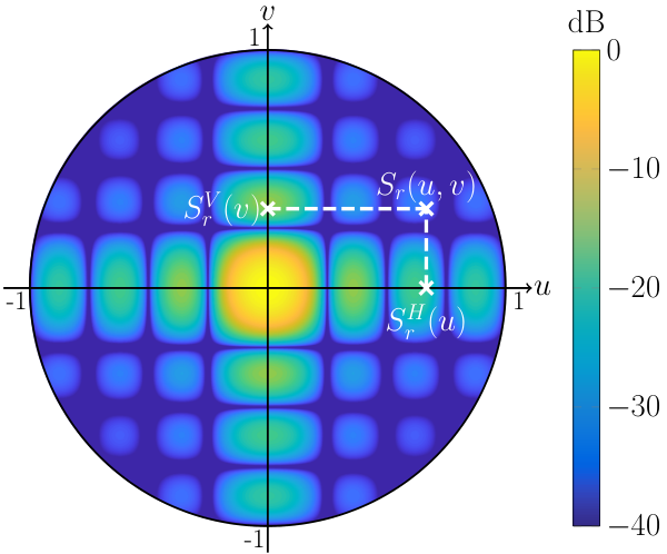
For correlated emissions the straightforward solution is to measure power flux density on a dense sphere, , which may result in very lengthy measurements. Two ways to reduce the measurement time have been identified. Either, the pattern lobes are narrow but the symmetries can be exploited, or the beams can be effectively widened by using a beam sweeping test signal. If the symmetries of the pattern is known, and the angular grid is aligned to the cardinal cuts, then an overestimate of the TRP is found. This is most probably the case for emissions at frequencies close to the operating band. Furthermore, if the symmetries of the antenna is known the power flux density pattern is well characterized by measuring two cardinal cuts, and then use \@iaciPM PM (PM) technique to retrieve values outside the cardinal cuts in order to get full sphere data. This is further described in the next paragraph, and the the beam sweeping test signal is further investigated in Sec. IV.
The proposed PM is based on the possibility to calculate the array factor of a rectangular array as a product of two terms, corresponding to two orthogonal cuts. Assuming an array positioned in the -plane, this must be done in two separate forward and backward hemispheres. Therefore, the data is separated in two hemispheres and the estimated radiated powers are added together. The two hemispheres are defined as33 3 Note that the factor is needed since a full turn is used for the vertical cut.
To exploit the rectangular array geometry, the PM uses the coordinates
| (18) |
The needed data are the horizontal and vertical power flux densities and , respectively. The power flux density in a point is calculated as
| (19) |
where is the power density at the crossover point. Note that power density at the crossover point is measured in both cuts and these values must be equal with a reasonable accuracy. The TRP is calculated as
| (20) | ||||
Where . Note that is singular at which must be taken care of in the integration, e.g. as shown in Appendix D.
To illustrate the PM method, an array of -oriented half-wave dipoles in the -plane is used. The radiation pattern of this array in the -plane is shown in Fig. 7 where the advantage of transformation to -plane is evident as well. If (14) is used an overestimation of almost 9 dB will result, whereas applying PM will reduce the error to virtually 0 dB.
IV Worst case configuration
For the TRP assessment of a device with many possible antenna configurations finding the worst case can be a practical difficulty. At different frequencies different configurations can lead to radiation in unpredictable directions with different levels of power. The only way to determine the worst configuration for each frequency would be to perform the measurement independently for each configuration in an exhaustive search manner. This can be a very time-consuming procedure. Even if the worst case configuration is known, it can be argued that this static state is not a representative mode for an AAS with dynamic beam forming and beam tracking capabilities.
As an illustration of unpredictable beam directions an example is provided. Assume an antenna array with 45 predefined beam positions on a grid. The beams span in the azimuth plane, in elevation and are uniformly spaced with between adjacent beams. The embedded radiation patterns of the antenna elements are obtained from FEM (FEM) simulations in the presence of nearest neighbor elements. Beam positions are studied at the second and third harmonics. In the absence of a complete model for out-of-band phase noise the same excitation is used at all frequencies. In Fig. 8 the location of the beam peaks are depicted using the embedded element pattern, the envelope of the steered beams, as background. In Fig. 9 the TRP of the beams are shown. The TRP values are normalized such that the mean value is at 0 dB for every frequency. It is observed that not only the peak directions, but also the index of the worst case beam is frequency dependent.


Instead of searching for and using a worst case configuration, a sweep through all the predefined beams can be used. During the measurement process the beam sweeping average of the radiated power flux density is measured at each measurement point. This averaging matches well with the fact that TRP is a spatial average of the measured values at different directions. Note, if instead the maximum value would be recorded for each point during the beam-sweeping, the resulting TRP estimate will be an overestimate by a wide margin. The resulting TRP value can afterwards be adjusted by a peak-to-average value which appears to be fairly similar for all frequencies as observed in Fig. 9.
The effect of using a beam sweeping test signal on the convergence of sparse sampling is shown in Fig. 10 as the error in TRP vs. , for full sphere and two cuts grids at the third harmonic. For both grids it is clear that the beam scanning test signal will result in smaller errors for larger which means that fewer number of samples can be used. This reduction in the number of samples, combined with the fact that only one configuration must be tested, will significantly reduce the total testing time. Regarding the two cut grid, it is noteworthy that the individual beams can lead to errors as large as 10 dB, while the beam scanning average leads to an overestimation error of almost 2 dB regardless of .
V Near-field radial power flux density
Near-field effects on TRP is divided in two parts. First, it is investigated in which spatial domain the far-field expression for radial power flux density (4) can be used. Secondly, the measurement errors associated with measurement of this quantity in the near-field region are discussed.
V-A Validity of far-field approximation
To evaluate the effect of using the far-field approximation of the radial power flux density (4), a back propagation technique based on \@iaciSWE SWE [8, 14, 15] is used. This method enables calculation of and fields including radial components, and using far-field data as input, see App. B and [8]. The fields can be calculated in any point excluding the zone where is on the order of . Hence, the SWE provides a tool to compare the true near field expression (3) and the far field approximation (4) of radial power flux density.
As a first example, a four column macro base station antenna with m at 2655 MHz is considered. 56 curves corresponding to four antenna ports and 13 different tilt settings are depicted in Fig. 11. The red triangles at and indicate the distances used in Figs 12 a-b showing the corresponding full sphere patterns. In this case, the far-field expression (4) can be used with an error below 0.065 dB all the way into 0.75 m. While a distinct sector beam appears in the far-field pattern, the near-field patterns have a different shape. While the radial power flux density is proportional to the only in the far-field pattern, at all distances m the far-field power flux density approximation (4) is close to the true expression (3). Note that by energy conservation the TRP is ideally independent of distance.
A second example depicts the TRP error for two antennas on a laptop as seen in Fig. 13. Since a comparison between the two antennas is not intended, the two are plotted with the same color at different frequencies. In this case a TRP error below 5% is achieved by using the far-field approximation at , and below 1% at . The far field distances are based on the mechanical dimensions of the laptop computer.
In a last example, arrays of vertical electric Hertz dipoles are used. The relative error in TRP is depicted in Fig. 14, and the relative error is below 0.05 dB at distances . As in the previous examples, the far field distance seems to be an irrelevant parameter when evaluating the error caused by using the far-field radial power flux density approximation (4) in the near-field.
Table II shows a comparison between the errors caused by back-propagation and those of the power flux approximation, for all the aforementioned examples. For each case the largest error is presented. The back propagation error is at least one order of magnitude smaller than the power flux approximation error, which verifies that the errors presented in Figs 11,13, and 14 are not numerical errors due to back propagation.
| Back propagation (dB) | Power flux density approximation (dB) | |
|---|---|---|
| base station antenna | 5.5e-3 | 6.5e-2 |
| notebook antenna | 2.6e-3 | 2.5e-1 |
| 1x4 array | 5.5e-6 | 2.8e-1 |
| 4x4 array | 5.3e-6 | 1.8e-3 |
| 8x8 array | 6.6e-5 | 6.1e-2 |
| 12x12 array | 1.1e-4 | 9.1e-2 |
V-B Measurement antenna considerations
The results of Sec. V-A imply that TRP can be assessed from if only the test distance exceeds by a few . To measure field data accurately, and the MA must be handled appropriately [16, 11]. To suppress influence from radial field components, the MA should be carefully aligned and the EUT should be placed in the far-field region of the MA. Furthermore, the HPBW (HPBW) of the MA shall cover the EUT, and to avoid influence from chamber scattering, excessive coverage shall be avoided [11]. Hence, using the relation [17] and the coverage criterion , cf. upper part of Fig. 15, implies that
| (21) |
Here is the width of the MA and for an open ended waveguide or SGH (SGH).
An alternative approach is based on the angular resolution of the EUT field. The received voltage at the MA port is modeled as the reaction integral [18]
| (22) |
Here is the equivalent electric current in the aperture and the integration is over the area of the antenna. If , cf. (26), then will be approximately constant over the aperture of the MA and will be proportional to the electric field strength. This is depicted in the lower part of Fig. 15 and leads to
| (23) |
(23) is a slightly stricter requirement than (21). Therefore, (23) is used hereafter. Note that (23) can be applied for any circular cut if , i.e. the radius of the smallest sphere enclosing the EUT. Moreover, it is noted that gives an upper bound to .
In the below examples \@iaciSWE SWE truncated by using , see App. B, is used for near-field calculations and [19] is used for modeling of the SGH aperture fields. The curvature of the field lines of is neglected corresponding to long flared sections of the horns. The voltage is calibrated to get a correct TRP value in the far-field of the EUT.
An array of vertical half-wave dipoles at 28 GHz, width 4.3 cm and height 30 cm is used. The exaggerated height-to-width ratio is chosen to increase the deviation of the near-field cut from the far-field. In Figs 16 and 17 probed power flux density using different widths is depicted. The radial cut of Fig. 16 is at the positive -axis. Minimum test distances (23) are indicated by dots, and the corresponding lines show small deviations at larger test distances. For the probe the minimum test distance is . It is observed that a can be used for power flux density measurement as close to the EUT as . Power flux density in the near field is not close to since EIRP is a far-field quantity. The horizontal cut of Fig. 17 is at and . At this distance, is suitable for measuring the power flux density. The intersection point of the cuts of Figs 16-17 is depicted by vertical black lines.
Finally, a link budget example for the accepted power at the MA port is given, see Fig. 18. The optimum width implies that the optimum effective area . According to (11) . Hence, the optimum is constant (dashed green curve), i.e. energy conservation. If a constant MA is used, is proportional to (solid green curve). As an example, the peak signal level is assumed constant near the EUT, and beyond some breakpoint . The peak accepted power, follows the same trend if a constant MA is used and the minimum test distance is respected (solid blue curve). Using an optimum MA yields proportional to close to the antenna and constant beyond the breakpoint (dashed blue curve). Note that the peak to average ratio, the antenna directivity in the far-field region, is reduced in the near-field. The maximum SNR (SNR) is achieved when the probe is used at the minimum test distance [11].
V-C Near-field impact on the TRP algorithm
Performance of some proposed TRP methods applied in the near-field and for the antenna used in Fig. 11 are shown in Fig. 19. The overestimation of the two cuts result is reduced at distances close to the EUT and PM performs well at all distances.
VI Conclusions
Challenges with OTA measurement of TRP in the MMW region have been addressed. These challenges are the angular resolution and the search for worst case antenna configuration.
For uncorrelated emissions, sampling can be used at the expense of adding margins up to dB. Different grid types, two or three orthogonal cuts of full sphere, can be used with no need for alignment of the measurement grid to the EUT. In the adjacent bands -plane pattern multiplication can be used on two-cut data to reduce uncertainty, both in far-field and near-field.
Secondly, a beam sweeping test signal is presented. Beam sweeping leads to wider beams for correlated emissions, e.g. emissions at harmonics, and therefore a more relaxed angular sampling can be applied. Beam sweeping will also reduce the number of test configurations to a single one. Furthermore, it is closer to real use conditions for devices with beam-forming and tracking capabilities.
Additionally, it has been demonstrated that near-field measurements of radial power flux density can be used for TRP assessment if the measurement antenna and test distance are selected by standard recommendations [11]. Other sources of error, e.g. alignment and field curvature effects, need further investigation.
Finally, for each finite test distance there is an optimal measurement antenna that will provide an average accepted power that is independent of test distance. Therefore, whether measurements need to be performed in the near-field is not fundamentally a question of path loss and signal levels, but rather a matter of measurement chamber size and equipment.
Appendix A Sampling criteria
The resolution needed to correctly characterize an electric, or magnetic, field component in a circular cut is presented in this section. Without loss of generality the cut is defined as the set and , i.e., a circle of radius in the -plane. Other circular cuts needed to cover a sphere are obtained by rotating the EUT. This field is periodic and can be expanded in the following series
| (24) |
where [8, Eq. (5.73)] and denotes rounding to nearest greater integer. A margin is commonly in use and corresponds to a dynamic range well above 40 dB in the measured data. Furthermore, is the radius of the smallest cylinder that encloses the EUT and has the -axis as symmetry axis. To demystify the subject of choosing , is rewritten in terms of wave number and distances as
| (25) |
It is noted that the margin can be interpreted as an added length resulting in an effective electrical length of the EUT. The extra length is on the order of one wave length, cf. [16, Fig. 10] where is used. The actual choice of or is related to the approximation error in Eq. (24). To accurately determine the coefficients , and indirectly the field , the angular sampling step needed is [8, Eq. (5.76)]
| (26) |
Note, is independent of and the circular cut can be taken anywhere in the radiating near-field or in the far-field region [8]. From the Parseval Theorem it follows that the angular average, which is the relevant quantity for TRP, is
This suggests that the sampling needed for a correct average value is . A major aim of this study is to investigate how densely angular measurements need to be taken in order to have a decent accuracy in the calculated TRP value. For this purpose the reference angular step is defined by using , resulting in
| (27) |
When the spherical coordinates (2) are used, the maximum radius in any constant cut is the radius of the smallest sphere enclosing the EUT, and the effective radius for the cuts is the radius of the smallest -directed and -axis centered circular cylinder that encloses the EUT [8]. Hence, the reference angular steps are defined as
Appendix B Spherical wave expansion
The electromagnetic fields of an antenna can be represented by a SWE (SWE) [8] as
| (28) |
and
| (29) |
where and is the radius of the smallest sphere enclosing the antenna, hence the SWE is valid both in the near-field and the far-field. The sums can be truncated at [8] where is the wave number, is the radius of the source, and is often chosen as 10. Furthermore, the radial functions are
where is the spherical Hankel function of the second kind, ensuring outgoing spherical waves. The angular functions are
where are Spherical harmonics and is the Nabla operator. Note the point-wise orthogonality between the tangential functions
| (30) |
Asymptotically as
Specifically for ,
| (31) |
These expressions can be used to compare the near-field and far-field approximation of power density for the modes and , i.e. a magnetic and electric infinitesimal dipole, see Fig. 21. For dipoles, it is seen that the far-field approximation, , is a good approximation as close as from the source. Since any antenna current can been represented as a super-position of dipole sources, this indicates that the approximation is probably valid also close to larger antennas. Note, when the form factor of EUT is not close to a sphere, only a small fraction of measurement points will be close. Hence, the effect of the TRP will be small.
The TRP of the SWE is calculated as
| (32) |
The SWE can be used to retreive near-field data from far-field data, i.e., back-propagation. The following procedure is used: Far-field data and is sampled on a full sphere. This data is used to calculate . Typically where the actual depends on the accuracy of the data and the desired precision. For evaluation at radius , the truncation limit is reduced to to control amplification of noise [15]. Electric and magnetic fields are then calculated by using (28) and (29), respectively. The back-propagation error is defined as the change in caused by the adaptive truncation.
Appendix C Rotations
A rotation matrix can be written as [20]
| (33) |
where the generator matrix
| (34) |
the rotation axis , and is the rotation angle in the positive sense around the rotation axis. Note that can be used to reduce the infinite Taylor series and identify the cosine and sine functions.
The far-field pattern for rotated point sources reads
| (35) |
To generate random rotations the rotation axis is parametrized using spherical coordinates, see (2),
| (36) |
and , are used to generate random rotations. Note that the rotation axis can be restricted to the upper hemi-sphere since .
Appendix D The -plane integration
As described in Sec. III the integration of eq. (20) involves a singularity along the edge of the visible region in coordinate system, i.e., . In order to resolve this singularity, the following change of variables is used
The infinitesimal solid angle is
Therefore, the radiated power in the forward hemisphere becomes
| (37) | ||||
where is the power flux density in the forward hemisphere. Finally, two test cases are given for code testing, see Table III. Test case (a) is separable in -coordinates, and therefore the PM estimate is identical to the true TRP.
| (a) | (b) | |
|---|---|---|
| @ | ||
| 1 | ||
Acknowledgment
The authors would like to thank the ANSI C63.26 working group, and Ericsson colleagues for fruitful discussions.
References
- [1] NR; Base Station (BS) radio transmission and reception, 3GPP Technical Specification (TS) TS 38.104 Release 15.
- [2] “Report and order and further notice of proposed rulemaking,” Federal Communications Commission (FCC), July 2016, FCC-16-89A1.
- [3] Electromagnetic compatibility (EMC) - Part 4-21: Testing and measurement techniques - Reverberation chamber test methods, International Electrotechnical Commission Std. IEC 61 000-4-21, Rev. Edition 2.0 2011-01.
- [4] P. S. Kildal, C. Orlenius, and J. Carlsson, “OTA testing in multipath of antennas and wireless devices with MIMO and OFDM,” Proceedings of the IEEE, vol. 100, no. 7, pp. 2145–2157, Jul. 2012.
- [5] D. A. Hill, “Electromagnetic theory of reverberation chambers,” National Institute of Standards and Technology (NIST), Radio-Frequency Division, Electronics and Electrical Engineering Laboratory, 325 Broadway, National Institute of Standards and Technology, Boulder, Colorado 80303, Technical Note 1506, Dec. 1998.
- [6] CTIA, “Test plan for wireless device Over-the-Air performance — method of measurement for radiated RF power and receiver performance,” Certification Program Test Plan, Nov. 2016, version 3.6.1. [Online]. Available: https://ctia.org/docs/default-source/certification/ctia-test-plan-for-wireless-device-over-the-air-performance-ver-3-6-1.pdf
- [7] American National Standard for Compliance Testing of Transmitters Used in Licensed Radio Services, ANSI Accredited Standards Committee C63® Electromagnetic Compatibility, ANSI C63.26-2015 Std., 2015.
- [8] J. Hald, J. E. Hansen, F. Jensen, and F. Holm Larsen, Spherical Near-Field Antenna Measurements, ser. IEE electromagnetic waves series, J. Hansen, Ed. Peter Peregrinus Ltd., 1998, vol. 26, edited by J.E. Hansen.
- [9] IEEE145-2013. IEEE Standard Definition of Terms for Antennas, Antenna Standards Committee of the IEEE Antennas and Propagation Society Std., Dec. 2013, approved Dec. 11.
- [10] D. K. Cheng, Field and Wave Electromagnetics, B. Rifkind, Ed. Addison-Wesley, 1989.
- [11] ANSI/IEEE Std 149-1979. IEEE standard test procedure for antennas, Antenna Standards Committee of the IEEE Antennas and Propagation Society, and American National Standards Institute Std., Dec. 1979, approved Aug. 8, 1980.
- [12] J. L. Allen, “Some extensions of the theory of random error effects on array patterns, chapter 3,” Lincoln Laboratory, Tech. Rep., 1960. [Online]. Available: https://www.researchgate.net/publication/235052482_PHASED_ARRAY_RADAR_STUDIES
- [13] J. Ruze, “Antenna tolerance theory — a review,” Proceedings of the IEEE, vol. 54, no. 4, pp. 633–640, April 1966.
- [14] S. Blanch, J. Romeu, and A. Cardama, “Near field in the vicinity of wireless base-station antennas: An exposure compliance approach,” IEEE Trans. Antennas Propagat., vol. AP-50, no. 5, pp. 685–692, May 2002.
- [15] J. Fridén, “RF exposure compliance boundary analysis of base station antennas using combined spherical-cylindrical near-field transformations,” IEE Electronics Letters, vol. 39, no. 25, pp. 1783–4, Dec. 2003.
- [16] A. Yaghjian, “An overview of near-field antenna measurements,” IEEE Transactions on Antennas and Propagation, vol. 34, no. 1, pp. 30–45, Jan 1986.
- [17] C. A. Balanis, Antenna Theory: Analysis and Design–2nd ed. John Wiley & Sons, Inc., 1997.
- [18] P.-S. Kildal, Foundations of Antenna Engineering. Kildal antenn AB, 2015.
- [19] H. J. Delgado and M. H. Thursby, “Implementation of the pyramidal-horn antenna radiation-pattern equations using Mathcad(R),” IEEE Antennas Propagat. Mag., vol. 41, no. 5, pp. 96–99, Oct. 1999.
- [20] Euler rotation theorem. [Online]. Available: http://en.wikipedia.org/wiki/Euler_rotation_theorem
![[Uncaptioned image]](1803.10993v2/Jonas.jpg) |
Jonas Fridén was born in 1965. He received the B.S. degree in mathematics and physics and the Ph.D. degree in theoretical physics from the University of Göteborg, Göteborg, Sweden, in 1987 and 1996, respectively. Since 2002, he has been with Ericsson Research, Ericsson AB, Göteborg, Sweden. In 1996 –1999, he was a lecturer with the College University of Borås. In 1999, he was with Ericsson Microwave Systems AB, where he worked with radar antennas, radar system, and radome design. He has also been a member of the European Electromagnetic Data Interface Group. His major areas of research are electromagnetic compliance, OTA measurement techniques, near field retrieval techniques, antenna theory, bandwidth limitations of antennas, and MIMO antenna system performance. |
![[Uncaptioned image]](1803.10993v2/Aidin.jpg) |
Aidin Razavi was born in 1982. He received the M.S. degree in microwave engineering from Tarbiat Modares University, Tehran, Iran, in 2007 and the Ph.D. degree from Chalmers University of Technology, Gothenburg, Sweden, in 2016. Between 2007 and 2009, he was with HT Telecom Co., Iran as senior engineer, and from 2009 to 2011 with Huawei Technologies Co., as radio network planning and optimization engineer. Since 2017, he has been with Ericsson Research, Ericsson AB, Göteborg, Sweden. His major areas of research include antenna theory, OTA measurements, MIMO antenna system performance, and optimal antenna apertures. |
![[Uncaptioned image]](1803.10993v2/Anders.jpg) |
Anders Stjernman was born in 1956. He received the M.S. degree in Physical Engeering from Lund University 1982 and Ph.D. degree in Space Physics from Umeå University 1995. Since 2002 he has been with Ericsson Research, Ericsson AB, Göteborg, Sweden. In 1995–2002, he was with Ericsson Microwave Systems AB, where he worked with radar antennas, radar system, radome design and bluetooth antennas. In 1986–1995 he worked at Swedish Institute of Space Physics (IRF) in Kiruna with radio remote sensing. His major areas of research are antenna theory, bandwidth limitations of antennas, and MIMO antenna system performance. |