Scalar Field Assisted Gravity Inflation
Abstract
In this paper we investigate the inflationary dynamics of an gravity in the presence of a canonical scalar field. We specifically choose the cosmological evolution to be a quasi-de Sitter evolution and also the gravity is assumed to be a modified version of the gravity. We investigate which scalar field potential can produce the quasi-de Sitter evolution for the choice of the gravity we made, and also we study in detail the inflationary dynamics of the resulting theory. As we demonstrate, the spectral index is identical to the one corresponding to the ordinary gravity, while the scalar-to-tensor ratio is found to be smaller than the inflation one consequently, compatibility with both the Planck 2015 and BICEP2/Keck-Array data is achieved.
pacs
04.50.Kd, 95.36.+x, 98.80.-k, 98.80.Cq,11.25.-wI Introduction
One of the most appealing scenarios of the early Universe is the inflationary scenario, which describes the abrupt nearly exponential accelerating expansion of the Universe in a quite small time interval. In modern theoretical cosmology, two of the most prominent trends in describing this early-time acceleration are the scalar field description [1, 2, 3] and the modified gravity description of inflation [4, 5, 6, 7, 8, 9, 10]. In both cases, various models of inflation were proposed from time to time, however after the latest Planck collaboration observational constraints [11], many models of inflation were disproved or severely constrained, see [12] for a recent review on this issue. In general there are various scalar-tensor models which remain viable even after the Planck data were released, for example the Starobinsky model [13, 14], the Higgs model [15] and a recently discovered class of scalar exponential models called -attractors [16, 17, 18]. Also, among various modified gravity theories, the gravity models combine an elegant simplicity with the successful confrontation with the Planck data, and also for the gravity description of the -attractor models, see [19, 20].
In view of the appealing properties of gravity and of the canonical scalar field inflationary models, in this paper we shall consider gravity in the presence of a canonical scalar field. This theory is the simplest form of an inflationary theory [9], so in this work we shall investigate how a scalar field affects the viability of a specifically chosen gravity. We shall assume that the gravity is a modified version of the model and we shall study the effects and implications of the scalar field on the observational indices. Our method is simple, since we will fix the Hubble rate to be a quasi-de Sitter evolution, and we shall find the form of the potential for which such an evolution is possible. Our main assumption for the gravity sector is that the slow-roll approximation holds true, and the same applies for the scalar field sector. With the present study we aim to provide a scalar-tensor assisted modified gravity model, which as we shall demonstrate remains viable, for a wider range of the parameter values, when the scalar-to-tensor ratio is considered.
The reasons for choosing a modified version of the gravity are firstly that any version of the gravity is functionally simple, and secondly the ordinary gravity yields inconsistencies when the term is considered, as we also discuss in the main text.
Thus in the next section, we study the modified inflationary scenario in the presence of a slow-rolling canonical scalar field. We realize a quasi-de Sitter Hubble rate, and we investigate which potential can assist the gravity to realize such an evolution. Also we calculate in detail the slow-roll indices and the corresponding observational indices and we confront the model with the observational data.
Before we proceed to the core of our article, we briefly present the geometric background we shall assume. Firstly, the metric will be assumed to be the flat Friedmann-Robertson-Walker (FRW), the line element of which is,
| (1) |
with being the scale factor. In addition, the metric connection is the Levi-Civita connection, which is torsion-less, metric compatible and symmetric.
II Slow-roll Scalar Field Assisted Modified Gravity
The theoretical framework which we shall consider in this article, is described by the simplest gravity, since it is an gravity in the presence of a canonical scalar field, with the action being,
| (2) |
and for simplicity we shall use a physical units system for which . By varying the gravitational action (2), with respect to the metric tensor, we obtain the cosmological equations of motion,
| (3) | ||||
| (4) |
with and the “dot” indicates as usual, differentiation with respect to the cosmic time . Also upon variation of the action (2) with respect to the scalar field , we obtain,
| (5) |
Our main interest in this paper is the inflationary dynamics, and the quantification of the dynamics is achieved by using the slow-roll indices , , which are defined as follows [21, 22, 23, 24, 25, 26, 9],
| (6) |
where the function appearing in Eq. (6) is defined as follows,
| (7) |
Also at this point we introduce the function , the analytic form of which is,
| (8) |
which will play a prominent role in the calculation of the scalar-to-tensor ratio.
Let us now assume that the functional form of the gravity is that of a modified model, that is,
| (9) |
where is for the moment a free parameter and also we shall assume that the Hubble rate is described by a quasi-de Sitter evolution,
| (10) |
The reason for choosing the modified version of the gravity, is the functional simplicity, but also there is another reason, as we discuss later on. In addition, both the gravity and the Hubble rate can be freely chosen, but this does not ensure that a viable inflationary era can be obtained. As we show later on, the choices (9) and (10) result to a viable inflationary era. Then, by using the gravitational equations (3), (4) and (5), we can find an approximate form for the scalar potential at leading order. Indeed, the potential as a function of the cosmic time is equal to,
| (11) |
So by substituting the functional form of and from Eqs. (9) and (10) and also taking into account that the scalar curvature for a FRW metric, during the slow-roll era is , the scalar potential at leading order in the cosmic time is,
| (12) |
From Eq. (4), by integrating the square root of it, we can find the function , which is,
| (13) |
At this point we shall explain the choice (9) in some detail. Actually, if we chose the ordinary gravity model, this would result to , which means that is not physical. Hence, the choice (9) was the simplest choice which would could make, and as we will show, it yields a viable inflationary cosmology, always in the presence of a canonical scalar field.
Let us proceed to the calculation of the potential, so by inverting (13) and substituting in Eq. (12), we obtain , which is,
| (14) |
So far the parameter appearing in the functional form of the gravity, namely Eq. (9), is left unidentified, however this will be fixed by requiring Eq. (5) to hold true for the solution (13) and for the potential (14). Since we assume that the scalar field is also slowly rolling down its potential, the term can be omitted in Eq. (5), but in any case, from Eq. (13), we can easily see that it is equal to zero. Hence the condition , fixes the value of at leading order, which is,
| (15) |
Now we turn our focus to the inflationary dynamics of the gravity in the presence of the scalar field. As we already indicated, we assume that the slow-roll approximation holds true in the gravity sector, and also the scalar field slowly rolls down its potential. In effect we expect that the second slow-roll index, namely in Eq. (6), is approximately zero. Remarkably though, a direct calculation results to the following equation,
| (16) |
which for the function and for the Hubble rate of Eqs. (9) and (10), the second slow-roll index is exactly equal to zero. Note that by using Eq. (16), we obtain not a leading order result, but an exact result for . If we calculate by using the solution appearing in Eq. (13), we would obtain a leading order result, so it would be less accurate. Let us proceed to the rest of the slow-roll indices appearing in (6), and we start off with and , which are found to be equal to,
| (17) |
and accordingly, the function is equal to , so the slow-roll parameter is equal to . Since all the slow-roll parameters satisfy the following condition , the spectral index of the primordial curvature perturbations can be calculated by the following formula,
| (18) |
so by substituting the resulting forms of the slow-roll indices, we obtain,
| (19) |
which is a function of the cosmic time. Accordingly, the function appearing in Eq. (8), is equal to,
| (20) |
The scalar-to-tensor ratio is equal to [9],
| (21) |
so by substituting (20), we finally get,
| (22) |
It is more convenient to express the cosmic time as a function of the -foldings number, and since we have the Hubble rate given, this can easily be done. Indeed, from the Hubble rate (10) and also by the condition , where is the time instance that inflation ends, we obtain
| (23) |
Also by using the definition of the -foldings number,
| (24) |
and by setting , we obtain,
| (25) |
By combining (23) and (25) we get the approximate relation between the -foldings and the time instance , which is,
| (26) |
Hence, by calculating the spectral index of primordial curvature perturbations (19) and also the scalar-to-tensor ratio (22), at the time instance and also by taking the large- limit, we obtain the observational indices,
| (27) |
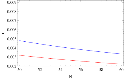
As it can be seen in Eq. (27), the spectral index is identical to the inflation case, however the scalar-to-tensor ratio is not the same, since in the case it is .
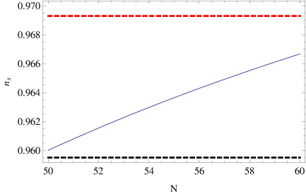
Hence, in the case at hand, the scalar-to-tensor ratio is smaller in magnitude. A striking feature is that the resulting observational indices are -independent, however this is possibly due to the model we used. In order to have a quantitative idea of the predictability of the model, let us give some characteristic values, for example if we choose , the spectral index becomes , and by direct comparison with the Planck data [11],
| (28) |
this means that it is within the allowed range of values for , which are . Also the scalar-to-tensor ratio for is , while the predicted scalar-to-tensor ratio for the model is , which is larger. In Fig. 1 we plot the behavior of the spectral index as a function of and in Fig. 2, we plot the scalar-to-tensor ratio for the modified model with scalar field (red curve) and for the model (blue curve). As it can be seen, in both cases, the values of the observational indices are well within the observational constraints of the Planck collaboration [11] but also within the allowed values of the BICEP2/Keck-Array data [27], which constrain the scalar-to-tensor ratio as follows,
| (29) |
Hence, as we demonstrated in this section, it is possible to obtain a viable slow-roll quasi-de Sitter evolution from an gravity which is not viable in vacuum, however in the presence of a scalar field with appropriately chosen potential, this theory becomes viable. In principle, other choice of gravity may be chosen, however if the gravity has a complicated functional form, analyticity is difficult to achieve and consequential approximations might be needed.
III Conclusions
In this paper we studied the simplest form of an gravity, and specifically an gravity in the presence of a canonical scalar field. We focused on the inflationary era and we assumed that the gravity has a specific form, leaving the scalar field theory free. Then, we fixed the Hubble rate of the cosmological evolution and we investigated which scalar potential can reproduce such a cosmological evolution in combination with the gravity. To this end, we assumed for both the and the scalar theory, the slow-roll conditions apply, that is , for the scalar field, and also and for the frame. Our calculations showed that the inflation in the presence of a scalar field leads to inconsistencies. So we introduced a variant form of the inflation, namely , and we found the potential of the scalar field that in conjunction with the modified gravity, realizes the quasi-de Sitter inflationary evolution. In addition, the value of the parameter was determined by using the slow-roll condition on the scalar field. For the resulting theory we calculated in detail the spectral index of primordial curvature perturbations and the scalar-to-tensor ration at leading order in the -foldings number , and as we demonstrated, compatibility with the Planck data but also with the BICEP2/Keck-Array data was achieved. Remarkably, the resulting theory is independent of the parameter , at least at leading order in .
An interesting issue which we did not address, but would be certainly interesting, is the study of the reheating era. This would be particularly interesting, since the presence of the scalar field can assist the reheating era, so this may directly affect the dynamics of the reheating era, and in effect may directly modify the reheating temperature. We hope to address this issue in a future work.
In principle, other choices for the Hubble rate and the gravity can be made, in order to obtain a viable inflationary cosmology. In this paper we made the simplest choices in order to obtain analytic results, at least in most of the cases.
Acknowledgments
Financial support by the Research Committee of the Technological Education Institute of Central Macedonia, Serres, under grant SAT/ME/170118-14/14, is gratefully acknowledged.
References
- [1] A. D. Linde, Lect. Notes Phys. 738 (2008) 1 doi:10.1007/978-3-540-74353-8_1 [arXiv:0705.0164 [hep-th]].
- [2] D. S. Gorbunov and V. A. Rubakov,“Introduction to the theory of the early universe: Cosmological perturbations and inflationary theory,” Hackensack, USA: World Scientific (2011) 489 p
- [3] D. H. Lyth and A. Riotto, Phys. Rept. 314 (1999) 1 doi:10.1016/S0370-1573(98)00128-8 [hep-ph/9807278].
- [4] S. Nojiri and S. D. Odintsov, eConf C 0602061 (2006) 06 [Int. J. Geom. Meth. Mod. Phys. 4 (2007) 115] doi:10.1142/S0219887807001928 [hep-th/0601213].
- [5] S. Capozziello and M. De Laurentis, Phys. Rept. 509 (2011) 167 doi:10.1016/j.physrep.2011.09.003 [arXiv:1108.6266 [gr-qc]].
- [6] V. Faraoni and S. Capozziello, Fundam. Theor. Phys. 170 (2010). doi:10.1007/978-94-007-0165-6
- [7] S. Capozziello, M. De Laurentis and V. Faraoni, Open Astron. J. 3 (2010) 49 doi:10.2174/1874381101003010049, 10.2174/1874381101003020049 [arXiv:0909.4672 [gr-qc]].
- [8] S. Nojiri and S. D. Odintsov, Phys. Rept. 505 (2011) 59 doi:10.1016/j.physrep.2011.04.001 [arXiv:1011.0544 [gr-qc]].
- [9] S. Nojiri, S. D. Odintsov and V. K. Oikonomou, Phys. Rept. 692 (2017) 1 doi:10.1016/j.physrep.2017.06.001 [arXiv:1705.11098 [gr-qc]].
- [10] T. Clifton, P. G. Ferreira, A. Padilla and C. Skordis, Phys. Rept. 513 (2012) 1 [arXiv:1106.2476 [astro-ph.CO]].
- [11] P. A. R. Ade et al. [Planck Collaboration], Astron. Astrophys. 594 (2016) A20 doi:10.1051/0004-6361/201525898 [arXiv:1502.02114 [astro-ph.CO]].
- [12] J. Martin, Class. Quant. Grav. 33 (2016) no.3, 034001. doi:10.1088/0264-9381/33/3/034001
- [13] A. A. Starobinsky, Phys. Lett. 91B (1980) 99. doi:10.1016/0370-2693(80)90670-X
- [14] J. D. Barrow and S. Cotsakis, Phys. Lett. B 214 (1988) 515. doi:10.1016/0370-2693(88)90110-4
- [15] F. L. Bezrukov and M. Shaposhnikov, Phys. Lett. B 659 (2008) 703 doi:10.1016/j.physletb.2007.11.072 [arXiv:0710.3755 [hep-th]].
- [16] R. Kallosh and A. Linde, JCAP 1307 (2013) 002 doi:10.1088/1475-7516/2013/07/002 [arXiv:1306.5220 [hep-th]].
- [17] S. Ferrara, R. Kallosh, A. Linde and M. Porrati, Phys. Rev. D 88 (2013) no.8, 085038 doi:10.1103/PhysRevD.88.085038 [arXiv:1307.7696 [hep-th]].
- [18] R. Kallosh, A. Linde and D. Roest, JHEP 1311 (2013) 198 doi:10.1007/JHEP11(2013)198 [arXiv:1311.0472 [hep-th]].
- [19] S. D. Odintsov and V. K. Oikonomou, Phys. Rev. D 94 (2016) no.12, 124026 doi:10.1103/PhysRevD.94.124026 [arXiv:1612.01126 [gr-qc]].
- [20] S. D. Odintsov and V. K. Oikonomou, arXiv:1611.00738 [gr-qc].
- [21] H. Noh and J. c. Hwang, Phys. Lett. B 515 (2001) 231 [astro-ph/0107069].
- [22] J. c. Hwang and H. r. Noh, Phys. Rev. D 65 (2002) 023512 doi:10.1103/PhysRevD.65.023512 [astro-ph/0102005].
- [23] J. c. Hwang and H. Noh, Phys. Lett. B 506 (2001) 13 doi:10.1016/S0370-2693(01)00404-X [astro-ph/0102423].
- [24] S. Nojiri, S. D. Odintsov and V. K. Oikonomou, Phys. Rev. D 94 (2016) no.10, 104050 doi:10.1103/PhysRevD.94.104050 [arXiv:1608.07806 [gr-qc]].
- [25] S. D. Odintsov and V. K. Oikonomou, Class. Quant. Grav. 33 (2016) no.12, 125029 doi:10.1088/0264-9381/33/12/125029 [arXiv:1602.03309 [gr-qc]].
- [26] S. D. Odintsov and V. K. Oikonomou, Phys. Rev. D 92 (2015) no.12, 124024 doi:10.1103/PhysRevD.92.124024 [arXiv:1510.04333 [gr-qc]].
- [27] P. A. R. Ade et al. [BICEP2 and Keck Array Collaborations], Phys. Rev. Lett. 116 (2016) 031302 [arXiv:1510.09217 [astro-ph.CO]].