The Eigenstate Thermalization Hypothesis and Out of Time Order Correlators
Abstract
The Eigenstate Thermalization Hypothesis (ETH) implies a form for the matrix elements of local operators between eigenstates of the Hamiltonian, expected to be valid for chaotic systems. Another signal of chaos is a positive Lyapunov exponent, defined on the basis of Loschmidt echo or out-of-time-order correlators. For this exponent to be positive, correlations between matrix elements unrelated by symmetry, usually neglected, have to exist. The same is true for the peak of the dynamic heterogeneity length , relevant for systems with slow dynamics. These correlations, as well as those between elements of different operators, are encompassed in a generalized form of ETH.
I Introduction
In recent years there has been a renewal of interest in chaotic systems within a quantum mechanical description. A characterization of wavefunctions is the Eigenstate Thermalization Hypothesis (ETH), an assumption that leads to a form for the matrix elements of local operators in the energy eigenbasis and can be viewed as an extension of ideas borrowed from random matrix theory. On the other hand, the Lyapunov exponent, a fingerprint of chaoticity in classical systems describing the sensitivity of the system’s dynamics to small perturbation [2], has been considered also for quantum systems based on the definition of suitable four point correlation functions. Both the applicability of the ETH to chaotic systems and the emergence of a Lyapunov exponent in their dynamics are subjects of active current research. The simultaneous consideration of these two aspects for non-integrable systems raises the question of how high order correlation functions are described within the ETH ansatz, the subject of this paper.
In the following we consider a hamiltonian which we assume is not integrable, and its eigenvalues . We assume that there is a parameter (e.g. or the number of degrees of freedom ) that controls the level spacing . Because timescales and energy are inversely related , this also defines the Heisenberg time , the longest in the system’s evolution (‘a theoreticians’s time’ [1]). Between the smallest microscopic time and the Heisenberg time are physical times where some correlations are non-zero [6]. Because the level density is in the semiclassical limit, both small and large may be cases where the separation of correlation and Heisenberg times is large, and we are thus allowed to consider an energy scale that contains many levels, but is much smaller than the energy corresponding to the inverse of all interesting physical times.
The Eigenstate Thermalization Hypothesis, as applied to expectation values [3, 4, 1, 7] is usually stated as follows: for the matrix elements of a smooth observable in the energy eigenbasis, putting :
| (1) |
where both and are assumed to be smooth functions of their arguments. For macroscopic systems, as we shall mostly consider here, we may assume that is a smooth function of the energy density. The origin of the factor comes from the spreading of weights over many levels, and is the only one compatible with of order one, as we shall see. The have expectation of order unity. Here we may consider that are real or complex hermitian. We have
| (2) |
Now, the off-diagonal elements are usually considered as independent random variables and therefore their product, apart from the obvious symmetries above, average to zero. Does this assumption together with (1) contain everything that is necessary to calculate -point functions? Clearly not, as this would ultimately mean that all higher correlation functions are obtainable as model-independent functionals of the one and two-point functions, i.e. all models would be Gaussian. In particular the correlations that determine the Lyapunov exponent [17, 13, 16, 2, 14, 15, 19], as well as the dynamic heterogeneities , are not fully included – and the most important physical part is indeed absent – in (1).
Let us now be more clear on what ensemble we have in mind when we say ‘random’. We may consider i) energies averaged over windows of extension in energy as above, ii) a perturbation , where is a local random Hamiltonian and the coupling is strong enough to couple nearby levels but sufficiently weak as to not affect correlation functions at physical times (see Deutsch [3]), iii) a set of transformations over physical observables described below (‘typicality’) (see [9, 10, 11, 12]). Denoting with an overbar averages over any of these ensembles, we may write:
| (3) |
where we have defined .
In the following sections we introduce and justify an ansatz for higher correlations, and we show how it applies to the calculation of the out of time order correlators (OTOC). We also give numerical support to the contention that the correlations between matrix elements are not negligible.
A convenient time-axis
Here we show how working on the shifted time-axis (and correspondingly, a split Gibbs measure in the trace) is the natural strategy [13, 18]. A way to introduce this construction is to consider two-point functions. The correlations and response functions are defined as (see e.g. [20]):
| (4) |
where we have made explicit . For :
| (5) |
It is easy to derive the so-called ‘KMS condition’ [5], the quantum version of fluctuation-dissipation relations, which in the time-domain may be expressed as a symmetry property:
| (6) |
for all . This strongly suggests that life becomes simpler if one displaces the -axis by and defines:
| (7) |
The KMS condition (6) is now the statement that is real, which is immediate from Hermiticity and the cyclic property of the trace:
| (8) |
We shall see the generalization of this below.
From matrix elements to correlations
Let us calculate for times small compared to the Heisenberg time the correlator Eq. (7), using the ansatz (1). We shall do this quickly here, and will justify the averaging involved in much more detail in the sections below.
| (9) |
We may hence change variables and . replacing sums by integrals (see e.g., Ref [1, 7])
| (10) |
and performing saddle point integration for (we are assuming a thermodynamic system), we obtain
| (11) | |||||
where is the canonical energy at temperature .
We first observe that the diagonal term must be of order one if is finite, while the scale is necessary so that the result is of order one, as it should. In conclusion, we find that the function is the Fourier transform of the correlation (7) which is defined along the shifted time axis. The usual correlation and response are obtained by shifting back the time-axis, and in so doing collecting a factor and , respectively [7]. Indeed, splitting the Gibbs measure gives a much simpler relation between time correlators and correlations between matrix elements, and this will be even more so in the sequel.
II Matrix elements and many-time correlation functions.
In Section III we shall show, using typicality considerations, that expectations of products of matrix elements in which indices are not repeated vanish. In this section we shall also argue that if an index is repeated more than twice, then the expectation breaks into a product of expectations. All in all, for the purposes of computing physical correlation functions, we shall only need to discuss the following generalization of (3) for different:
| (12) |
where and is a smooth function of the energy differences and a a smooth function of the average energy density . The factor:
| (13) |
guarantees that is of order one. Averages are as above. Expression (12) contains (3) as a particular case for . A similar expression may be expected to hold if the matrices are different (e.g. ), with an appropriate function dependent on the operators involved.
Note that the usual ETH assumes an absolute value of the ’s of the order , while the part contributing to higher correlations is much smaller: per factor. These correlations between matrix elements are indeed smaller, but enter all expressions for -point time-correlations through sums with many more terms, so that their contribution to physical correlation functions is of the same order – just as what happens between diagonal and off-diagonal terms in (3). Indeed, as we shall see explicitly in the next subsections, a sum over indices of the average (12) picks up a factor from the density of levels, while we may estimate the sum of the (larger) fluctuating parts as being only a factor , due to random signs.
We have restricted ourselves to different indices. In fact, when there is a repetition one can see that what dominates are products of lower order expectations under some assumptions on the fluctuating parts.. Consider, for example the case in which , and all other indices are different:
| (14) |
where we have splitted into average and fluctuating parts and . We assume that the average of fluctuating parts scales at most like (12) (i.e. as the result without index repetitions). We wish to compare this with the product of averages, which contain and terms, respectively. Put and , so that: . The size of the estimate (12) is the exponential of
| (15) |
where in the inequality we have used the convexity of (itself a consequence of the positivity of specific heat). This is to be compared with the estimate for the logarithm of the product:
| (16) |
Using the fact that and are nonnegative, we check that the product form always dominates
| (17) |
In short, and are stochastic variables whose expectations factorize up to exponential accuracy if their covariances scale as (12) . Their variances are always large, but contribute subdominantly to the sums over indices involved in the calculation of correlation functions.
Proceeding this way, one may use this argument to generalize (17). In particular, the fact that the ansatz (12) is all we need to calculate point correlations may be argued as follows. Consider a product . We may represent it as a diagram by using as vertices all the different indices amongst the set . Each factor is then represented by an arrow (for complex , real are represented by a simple edge) going from to . We consider: i) the simplest non-zero expectation, the one involved in ansatz (12) corresponds to a diagram with all distinct vertices lying on a single loop. ii) Next, we consider a tree of loops, joined to one another at single vertices: a ‘cactus’ diagram (a two-leaf cactus is (17)). The entropic argument (15) may be generalized (see Appendix B) to argue that the expectation of such a product is dominated by a product of its constituent loops, each obtained from (12), under the assumption that the covariaces scale as (12). This is the generalization of (17). iii) Finally, we have products that are non cacti, for example . These products may be decomposed in loops in more than one way (for example . For these we make the assumption that their order in is the same as the one of the decomposition in loops that dominates. These expectations may be large in order, but they have less free indices that the corresponding cactus, and hence pick up less factors and their contribution to the n-point correlation functions is subdominant. In Fig. 4 and Fig. 6 we show examples of loops, cactus and non-cactus products. We shall not discuss the averages of non-cactus products here, but let us note that we need to calculate them if we wish to determine the whole probability distribution , through expectations of the moments .
Correlations
The functions are closely related to the time correlations [13]:
| (18) | |||||
which clearly depend only on time-differences. (From here onwards we set ). Time correlations are invariant with respect to cyclic permutations of indices, a translation of all times , and satisfy the ‘KMS’ condition (the generalization of (8)):
| (19) |
The ordinary -point correlations and responses can be obtained by analytic continuation. Shifting the various times by a suitable imaginary amount:
| (20) |
Let us consider, for the moment, the partial sum of (18):
| (21) |
Eq. (19) clearly implies also that and
| (22) |
We also consider the Fourier transform:
| (23) |
which may be written as:
| (24) | |||||
Eq. (24) describes a function made of many deltas of random amplitudes, a ‘comb’. The definition implies no assumption. If we now perform an average of the operators in the spirit of a typicality argument (see next section) we obtain, assuming (12):
| (25) | |||
| (26) |
Smoothing over a scale of many eigenvalues, but small energy difference , replacing sums by integrals (see e.g., Ref [1, 7]) , and performing saddle point integration for , we obtain
| (27) |
where is the canonical energy at temperature , associated with the partition function . This justifies the choice made for , that precisely cancels the levels density. In going from (10) to (27) we have used that:
| (28) | |||||
where we have used that the quadratic and higher terms in become negligible – see argument leading to (210) in [7]. Note the simplifying role of using a split Gibbs-Boltzmann factor, guaranteeing the cancellation of terms linear in .
We can also write
| (29) |
where the sign means that the approximate equality holds for times , so that the Fourier transform implicitly smooths the amplitudes of the delta peaks in Eq. (24) and we may replace by : this allows us to write the equation for without any other averaging.
In order to reconstruct the complete time correlation (18), we need to consider all the different possible ways in which indices may coincide. We shall do this in detail for three and four point functions below, let us state here the basic principle. Suppose we are calculating:
| (30) | |||||
as in (14). We may replace this by the product average (17) and compute everything in terms of lower correlation functions. Another way of doing this is to observe that the if we add in (18) to the times , this produces a modification only in a factor . Letting will produce a rapidly oscillating factor whose contribution will cancel through random phases – the usual argument for the diagonal approximation. Hence, we may make the association , and:
| (31) |
As a final remark, let us mention that if is an observable satisfying ETH, consistently, also should also be. Let us here only argue that the -element correlations of contribute to :
| (32) | |||||
so we see that definitely has a contribution to the diagonal part of a power of matrices. The full closure of the forms of expectations under matrix products is an interesting question to check in detail, but we shall do this in a future work.
III ‘Typicality’ of operators
In this section we use ‘typicality’ arguments to justify the claim made above, that only expectations with every index repeated are non-zero.
III.1 Two-point functions
Consider a situation where would be a full complex Hermitean matrix, in the basis of the Hamiltonian (i.e., the function would be a constant). A notion of ‘typicality’ that goes back to Von Neumann [9], and further discussed in [10, 12] (here we follow [11]) is to assume that may be replaced by , with a Gaussian random matrix, without altering results such as correlations. The group associated with depends on the symmetry of : if it is complex hermitean the is a unitary matrix, while if is real it is orthogonal. We shall here restrict ourselves to the unitary case, the generalization to orthogonal or symplectic cases is straightforward.
This typicality cannot apply for rotations in the entire Hilbert space in reality, because they would destroy the band structure given by that determines the time-correlation functions, but let us ignore this for the moment. We can then evaluate the correlation function as an average over using:
| (33) |
where are related to the invariants of the matrix, and .
Clearly, one may generalize this to point functions [11]:
| (34) |
where we assumed implicit summation over repeated indices. For the unitary group [21, 11]
| (35) |
where are all permutations and known combinatorial numbers. Therefore:
| (36) |
The matrix then enters in the average only through its invariants , implicitly defined above. Terms which are not invariant under rotation would be in fact be modified by averaging. For , for instance, there are two terms proportional to and which for the particular case of Eq (33) reduces to and to .
In our case, we have to deal with averages of the particular kind:
| (37) |
where the are functions of the invariants of the matrix . Clearly, the product impose the equalities of indices in groups. For example imposes the equality of all indices, while imposes nothing.
Now, suppose we wish to compute using the ‘typicality’ of operators a quantity like (21), for the moment still for the case of a ‘full’ random matrix. We should inject (37) into (18).
| (38) |
For the case , equation (38) reads:
| (39) |
where we have explicitly put all diagonal contributions in the second term.
It is clear then, comparing with (1), what we are missing in this first ‘typicality’ approach: we need to impose the fact that local operators may be ‘typical’ with respect to rotations between eigenstates associated with nearby levels, but ‘in the large’ they have a band structure given by , which so far is absent. One way to accomplish this [3] has already been mentioned above: it is to add to the Hamiltonian a small () random perturbation that will effectively mix level within a range of energy . We follow here a slightly different route [11]. Let us then consider a realistic system, where there is concentration of matrix elements near the diagonal. Imagine for example we wish to estimate which of the products have a non-zero expectation value. We first introduce an energy scale such that it contains many levels, but is small in the thermodynamic limit (or, in a semiclassical one). A modified form of typicality may be introduced as follows: consider the energy intervals
| (40) |
and let us first assume that they are disjoint. We now define a group of unitary matrices of the form Fig. 1, where are independent matrices.
We now assume that there is typicality within this group, i.e
| (41) |
The average is clearly zero, because each rotation is independent. In order to have the possibility of a non-zero average, we need that a matrix appears at least twice, once conjugated. For this to happen, we need that the indices be at most in two intervals. Consider the case when belong to an interval, and to another, and the rotations associated with these two sets are and respectively. We have then:
| (42) |
Here and in the following the argument ‘(intervals)’ makes explicit the fact that the constant is dependent on where are located the intervals considered by the rotations – i.e. a function of the energies defining (up to a small uncertainty ) the two intervals. The other possibility is that belong to an interval, and to another. Then, we have:
| (43) |
a product diagonal terms. This means that the non-zero expectation is:
| (44) |
The normalization is for the moment arbitrary. We set it to so that remains of order one. For the first term we assume that may be at most of order one, corresponding to an operator having a finite limit for its large-time two-point function.
III.2 Three-point functions
Consider first a term like: or, in particular, . The energies may be contained in at most intervals of size . If we proceed as before, with rotation along at most intervals around the indices, we find as before that in order to have a non-zero average, a rotation must appear at least twice, one affecting a first and one affecting a second index. This means that we need to restrict ourselves to indices such that the are contained in the same intervals. In order to see how these averages work, let us develop in detail the case .
Our unitary matrix ensemble is as in Fig. 1. In column to the left of Fig 2 we show the combinatorics of the energy intervals. Next, averaging over the independent transformations for every interval, we obtain a number of delta functions imposing some equalities of indices. The diagrams on the right have a full line if indices coincide, a dashed line if they do not coincide but are in the same energy block, and no line when they are in different blocks.
- •
If two indices are different , but they belong to the same interval, this means that : they are very close in terms of the parameters of the problem , but do not coincide.
- •
If two indices are at different intervals, we assume that the average over the combined rotations depends smoothly on the energies , .
Typicality with respect to random unitary transformation of this kind implies that matrix elements products involving eigenstates associated to eigenvalues that are neighbours or differ by a few level-separations may be completely different from matrix elements products containing the diagonal elements. This is already so in the original ETH ansatz, where the diagonal elements scale differently (have a large expectation value) from the off-diagonal elements .
Going back to the diagrams 2, the situation is summarised as follows: putting :
- •
in different blocks (diagram (a)) then
(45) where is a smooth function of fixed so that is of . We shall determine it below.
- •
Whenever two energies are different but are in the same block, we assume that the corresponding matrix element is simply given by a limit of Eq (45). For example,
(46) This is natural, since the size of the intervals is many level-separations but otherwise arbitrary.
- •
If two indices coincide – there is a full line in the diagram – then the elements may scale in a different way, and their form is not obtained as a limit of .
All in all, the situation is reduced to Figure 3, with a scaling function for each set of indices that differ. We can now write, for times that are smaller than the Heisenberg time, so that we may replace the matrix products by their averages:
| (47) | |||||
In direct correspondence with the diagrams of Fig 3 (we have not made explicit the supraindex (a) for the function corresponding to all indices different: it will be understood by default). Here and in what follows, a bar over means that the sum is unrestricted, while a without a bar assumes all indices are different, unless they have explicitly the same name.
As mentioned above, to clarify the role of the sum over repeated indices in the time domain, consider the limit of times larger than the Heisenberg time: . From equation (18) we see that the rapidly oscillating factors will cancel everything by random phases, except the diagonal terms with . Hence
| (48) |
(a)
(b)
(c)-(d)-(e)
III.3 Four-point functions
(a)
(b)
(c)
(d)
(e)
(f)
(g)
We shall consider also the -point function, as it is the one that is used to define the Lyapunov exponent and the Dynamic Heterogeneity length [24]:
| (49) | |||||
We now wish to express (49) as a sum of terms with all possible index contractions, i.e. corresponding to the diagrams in Fig 5. Let us first consider the sum with all indices different, corresponding to diagram (a):
| (50) |
or its Fourier transform
| (51) |
Again, the difference between and is that is a ‘comb’ of delta-functions, while is a version that has been smoothed either by averaging over an energy window or by averaging over unitary transformations as described above. Eq. (12) is, for the case of four different indices:
| (52) |
IV The Lyapunov exponent and the out of time order correlator
The Lyapunov exponent is derived from the OTOC by assuming [13] that there is a time regime, larger than the correlation time, such that:
| (53) |
for times , where is (an estimate of) the Ehrenfest time, the time taken for a minimal packet to spread throughout phase-space [13, 22, 8] (for a detailed discussion of the connections between the fidelity decay and the Lyapunov exponent, see Ref. [2, 19]). The quantum exponent extracted from the OTOC coincides with the classical one in some instances of the semiclassical limit [22], but this is not necessarily the case [23]. It should be also noted in passing, as implicitly stated in Ref. [23], that the Lyapunov exponent so-defined corresponds to an average taken before the logarithm, and not after as is the normal definition: in the language of disordered systems it is an ”annealed” rather than a ”quenched” average.
The terms contributing to the OTOC can be separated in those resulting from different sums over indices, corresponding to diagrams of Fig 5. As we have seen above, the only term that is not directly deducible, with a model-independent 11 1 This might seem confusing, as in spin-glass models, and in particular SYK model, the four-point function is a functional of the two-point functions. Note, however, that this dependence depends on the model and its parameters, it is not simply a variant of clustering formulas formula (see below) from two or three-point correlation functions 22 2 The latter we assume is zero by symmetry. is the sum with all indices different, so we expect that the exponential growth is given by this term:
| (54) |
a real, even function of time. In Fourier space it reads:
| (55) |
The smoothed version of this reads:
| (56) |
What to expect of the general features of (56)? First of all, because is expected to be nonzero for times smaller than the Ehrenfest time, this means that should be smooth on a scale (by which we mean that convoluted with a Gaussian having a width smaller than that, it remains unaltered). We expect, however, oscillations of , if extends to . The information we seek is in the envelope of these oscillations.
A rapidly oscillating function suggests that one has to study it for complex variables, which leads us to compute the Laplace transform:
| (57) | |||||
| (58) |
In the last equality we have substituted the function for the smoothed version, a safe thing to do for much larger than the level spacing.
The function is analytic outside the imaginary axis (cfr Eq (57)) for finite. However, in the limit of diverging Ehrenfest time, a form (53) implies that has a pole in zero (rounded off at a scale ) and a pole in of residue , rounded off at a scale . The rounding-off of poles re-establishes analyticity for finite.
The bound to Lyapunov [13] means that is analytical for .
IV.1 Numericals results
Following [7], we compute the correlation functions of a one-dimensional model of hard-core bosons with the Hamiltonian
| (59) |
The number of bosons was set to be . The three terms in this Hamiltonian describe, from left to right, hopping, dipolar interactions, and a harmonic potential. Here, is the distance of site from the center of a trap. For , this model is non-integrable.
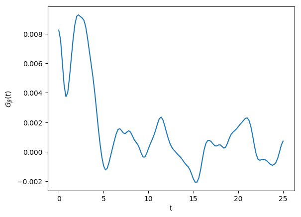
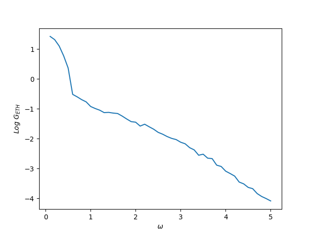
Figure 7 shows the function computed for a system of size where we considered as an observable the site occupation at the center of the chain, and Fig 8 shows its Fourier transform. The sizes are small, but we clearly see correlations that are absent in the usual assumption of independence of matrix elements unrelated by symmetry. Figure 9 shows the contribution of the all terms except the ones in Fig. 7: we see a behaviour very close to that of the two-point function computed in Ref [7].

V Conclusions
We have argued that that matrix elements of local operators in the basis of a chaotic Hamiltonian retain correlations that are small but contribute to higher correlation functions. The set of nonzero expectations of products of matrix elements is in a one-to-one relation with the set of connected correlator. Even if the ETH ansatz with independent elements may be shown to close under products [1, 7], so that, for example, the square of an operator of the ETH form is also of the ETH form, the neglected correlations between elements contribute and disregarding them may lead to incorrect results. A simple argument to convince oneself of this is that, if expectations of diagonal and variances of off-diagonal elements sufficed to determine all -time correlations, then all could be written as model-independent functional of one and two-time correlations, which is for general models obviously not the case. An interesting generalization of the present work is to derive ETH forms for the joint distribution of various operators, under the same assumptions of this paper.
VI Acknowledgments
We acknowledge M. Rigol and Y. Kafri for useful discussions. L.F. and J.K. are supported by the Simons Foundation Grant No 454943.
Appendix A Contributions from other diagrams
The other contributions to associated to the diagrams in Fig. 5 derive from the 2-point function within the standard ETH or its extension for the three point function:
| (60) |
where we made the change of variables ,
| (61) |
with
| (62) |
with
| (63) |
with
The diagram corresponds to a diagram that is not a cactus and therefore does not contribute (see comment in Sec. II). Finally one has:
| (64) |
Appendix B Counting argument
Let us consider a loop with repetitions characterized by . This is partitioned in subloops of sizes and energies with . We define , with , , and . It holds:
| (65) |
where in the first inequality we have used the convexity of the entropy and in the second the fact that . Therefore, if we assume that the covariances of such loops (and their generalization to multi-point functions) scale as we see that the expectation of the maximal contraction in loops dominates the expectation of the diagram.
References
- [1] M. Srednicki, J. Phys. A 32, 1163 (1999).
- [2] A. Goussev, R. A. Jalabert, H. M. Pastawski and D. A. Wisniacki, .
- [3] J. M. Deutsch, Phys. Rev. A 43, 2046 (1991).
- [4] M. Srednicki, Phys. Rev. E 50, 888 (1994).
- [5]
R. Kubo, J. Phys. Soc. Jap. 12 (1957) 570
P. C. Martin and J. S. Schwinger, Phys. Rev. 115 (1959) 1342. - [6] Note that the dynamics are not frozen after the Heisenberg time, instead the fidelty can undergo a dephasing dynamics beyond that time, see Ref. [19].
- [7] L. D’Alessio, Y. Kafri, A. Polkovnikov and M. Rigol, Advances in Physics Vol. 65 , Iss. 3, (2016).
- [8] The possibility has been raised that the work in: Ruch, E. and Mead, A. Theoret. Chim. Acta (1976) 41: 95, might be relevant to this discussion (communication by an anonymous referee), we have not as yet been able to work this out.
- [9] J. von Neumann, Z. Phys. 57, 30 (1929). [English translation: R. Tumulka Eur. J. Phys. H 35, 201 (2010) ].
- [10] S. Goldstein, J. L. Lebowitz, C. Mastrodonato, R. Tumulka and N. Zanghì Phys. Rev. E 81 011109 (2010).
- [11] P. Reimann, Nat. Commun. 7, 10821 (2016).
- [12] P. Reimann, New J. Phys. 17, 055025 (2015).
- [13] J. Maldacena, H. S. Shenker and D. Stanford, Journal of High Energy Physics 8, 106 (2016).
- [14]
A. Peres, Phys. Rev. A 30.4, 1610 (1984),
R. A. Jalabert and H. M. Pastawski, Phys. Rev. Lett. 86.12, 2490 (2001). - [15]
See: T. Gorin, T. Prosen, T. H. Seligman and M. Znidaric, Phys. Rep. 435, 33-156 (2006), and references therein;
J. Vanicek and E. J. Heller, Phys. Rev. E 68.5, 056208 (2003). - [16] A. Kitaev, “A simple model of quantum holography.” http://online.kitp.ucsb.edu/online/entangled15/kitaev/,http: //online.kitp.ucsb.edu/online/entangled15/kitaev2/. Talks at KITP, April 7, 2015 and May 27, 2015.
- [17] A. I. Larkin and Y. N. Ovchinnikov, JETP 28, 1200 (1969).
- [18] F. M. Haehl, R. Loganayagam, P. Narayan, A. Nizami and M. Rangamani,, Journal of High Energy Physics 12 154 (2017).
- [19] T. Prosen, M. Znidaric, Journ. of Physics A: Mathematical and General, 35 1455 (2002)
- [20]
A. Kamenev, Field theory of non-equilibrium systems,
Cambridge University Press (2011);
G. Mahan, Many-particle physics, (2013), Springer Science & Business Media. - [21] P. W. Brouwer and C. W. J. Beenakker, J. Math. Phys. 37, 4904 (1996)
- [22] J. Kurchan, arXiv:1612.01278v2, J. J Stat Phys (2018) 171: 965.
- [23] E. B. Rozenbaum, S. Ganeshan, V. Galitski, Phys. Rev. Lett. 118(8), 086801 (2017)
- [24] Berthier, Ludovic and Biroli, Giulio and Bouchaud, Jean-Philippe and Jack, Robert L, Dynamical Heterogeneities in Glasses, Colloids, and Granular Media, 150, (2011), Oxford University Press New York.