Bayesian Regression with Undirected Network Predictors with an Application to Brain Connectome Data
Abstract
This article proposes a Bayesian approach to regression with a continuous scalar response and an undirected network predictor. Undirected network predictors are often expressed in terms of symmetric adjacency matrices, with rows and columns of the matrix representing the nodes, and zero entries signifying no association between two corresponding nodes. Network predictor matrices are typically vectorized prior to any analysis, thus failing to account for the important structural information in the network. This results in poor inferential and predictive performance in presence of small sample sizes. We propose a novel class of network shrinkage priors for the coefficient corresponding to the undirected network predictor. The proposed framework is devised to detect both nodes and edges in the network predictive of the response. Our framework is implemented using an efficient Markov Chain Monte Carlo algorithm. Empirical results in simulation studies illustrate strikingly superior inferential and predictive gains of the proposed framework in comparison with the ordinary high dimensional Bayesian shrinkage priors and penalized optimization schemes. We apply our method to a brain connectome dataset that contains information on brain networks along with a measure of creativity for multiple individuals. Here, interest lies in building a regression model of the creativity measure on the network predictor to identify important regions and connections in the brain strongly associated with creativity. To the best of our knowledge, our approach is the first principled Bayesian method that is able to detect scientifically interpretable regions and connections in the brain actively impacting the continuous response (creativity) in the presence of a small sample size.
Keywords: Brain connectome; Edge selection; High dimensional regression; Network predictors; Network shrinkage prior; Node selection.
1 Introduction
In recent years, network data has become ubiquitous in disciplines as diverse as neuroscience, genetics, finance and economics. Nonetheless, statistical models that involve network data are particularly challenging, not only because they require dimensionality reduction procedures to effectively deal with the large number of pairwise relationships, but also because flexible formulations are needed to account for the topological structure of the network.
The literature has paid heavy attention to models that aim to understand the relationship between node-level covariates and the structure of the network. A number of classic models treat the dyadic observations as the response variable, examples include random graph models (Erdos and Rényi, 1960), exponential random graph models (Frank and Strauss, 1986), social space models (Hoff et al., 2002; Hoff, 2005; Hoff, 2009) and stochastic block models (Nowicki and Snijders, 2001). The goal of these models is often either to predict unobserved links or to investigate homophily, i.e., the process of formation of social ties due to matching individual traits. Alternatively, models that investigate influence or contagion attempt to explain the node-specific covariates as a function of the network structure (e.g., see Christakis and Fowler, 2007; Fowler and Christakis, 2008; Shoham et al., 2015 and references therein). Common methodological approaches in this context include simultaneous autoregressive (SAR) models (e.g., see Lin, 2010) and threshold models (e.g., see Watts and Dodds, 2009). However, ascertaining the direction of a causal relationship between network structure and link or nodal attributes, i.e., whether it pertains to homophily or contagion, is difficult (e.g., see Doreian, 2001 and Shalizi and Thomas, 2011 and references therein). Hence, there has been a growing interest in joint models for the coevolution of the network structure and nodal attributes (e.g., see Fosdick and Hoff, 2015; Durante et al., 2017; De la Haye et al., 2010; Niezink and Snijders, 2016; Guhaniyogi and Rodriguez, 2017).
In this paper we investigate Bayesian models for network regression. Unlike the problems discussed above, in network regression we are interested in the relationship between the structure of the network and one or more global attributes of the experimental unit on which the network data is collected. As a motivating example, we consider the problem of predicting the composite creativity index of individuals on the basis of neuroimaging data reassuring the connectivity of different brain regions. The goal of these studies is twofold. First, neuroscientists are interested in identifying regions of the brain that are involved in creative thinking. Secondly, it is important to determine how the strength of connection among these influential regions affects the level of creativity of the individual. More specifically, we construct a novel Bayesian network shrinkage prior that combines ideas from spectral decomposition methods and spike-and-slab priors to generate a model that respects the structure of the predictors. The model produces accurate predictions, allows us to identify both nodes and links that have influence on the response, and yield well-calibrated interval estimates for the model parameters.
A common approach to network regression is to use a few summary measures from the network in the context of a flexible regression or classification approach (see, for example, Bullmore and Sporns, 2009 and references therein). Clearly, the success of this approach is highly dependent on selecting the right summaries to include. Furthermore, this kind of approach cannot identify the impact of specific nodes on the response, which is of clear interest in our setting. Alternatively, a number of authors have proceeded to vectorize the network predictor (originally obtained in the form of a symmetric matrix). Subsequently, the continuous response would be regressed on the high dimensional collection of edge weights (e.g., see Richiardi et al., 2011 and Craddock et al., 2009). This approach can take advantage of the recent developments in high dimensional regression, consisting of both penalized optimization (Tibshirani, 1996) and Bayesian shrinkage (Park and Casella, 2008; Carvalho et al., 2010; Armagan et al., 2013). However, this approach treats the links of the network as if they were exchangeable, ignoring the fact that coefficients that involve common nodes can be expected to be correlated a priori. Ignoring this correlation often leads to poor predictive performance and can potentially impact model selection.
Recently, Relión et al., 2017 proposed a penalized optimization scheme that not only enables classification of networks, but also identifies important nodes and edges. Although this model seems to perform well for prediction problems, uncertainty quantification is difficult because standard bootstrap methods are not consistent for Lasso-type methods (e.g., see Kyung et al., 2010 and Chatterjee and Lahiri, 2010). Modifications of the bootstrap that produce well-calibrated confidence intervals in the context of standard Lasso regression have been proposed (e.g., see Chatterjee and Lahiri, 2011), but it is not clear whether they extend to the kind of group Lasso penalties discussed in Relión et al., 2017. Recent developments on tensor regression (e.g., see Zhou et al., 2013; Guhaniyogi et al., 2017) are also relevant to our work. However, these approaches tend to focus mainly on prediction and identification of important edges, but are not designed to detect important nodes impacting the response.
The rest of the article evolves as follows. Section 2 proposes the novel network shrinkage prior and discusses posterior computation for the proposed model. Empirical investigations with various simulation studies are presented in Section 3, while Section 4 analyzes the brain connectome dataset. We provide results on region of interest (ROI) and edge selection and find them to be scientifically consistent with previous studies. Finally, Section 5 concludes the article with an eye towards future work.
2 Model Formulation
Let and represent the observed continuous scalar response and the corresponding weighted undirected network for the th sample, respectively. All graphs share the same labels on their nodes. For example, in our brain connectome application discussed subsequently, corresponds to a phenotype, while encodes the network connections between different regions of the brain for the th individual. Let the network corresponding to any individual consist of nodes. Mathematically, this amounts to being a matrix, with the th entry of denoted by . We focus on networks that contain no self relationship, i.e., , and are undirected (). The brain connectome application considered here naturally justifies these assumptions. Although we present our model specific to these settings, it will be evident that the proposed model can be easily extended to directed networks with self-relations.
2.1 Bayesian Network Regression Model
We propose the high dimensional regression model of the response for the -th individual on the undirected network predictor as
| (1) |
where is the network coefficient matrix of dimension whose th element is given by and denotes the Frobenius inner product between and . The Frobenius inner product is the natural inner product in the space of matrices and is a generalization of the dot product from vector to matrix spaces. Similar to the network predictor, the network coefficient matrix is assumed to be symmetric with zero diagonal entries. The parameter is the variance of the observational error. Since self relationship is absent and both and are symmetric, . Then, denoting , (1) can be rewritten as
| (2) |
Equation (2) connects the network regression model with the linear regression framework with ’s as predictors and ’s as the corresponding coefficients. However, while in ordinary linear regression the predictor coefficients are indexed by the natural numbers , Model (2) indexes the predictor coefficients by their positions in the matrix . This is done in order to keep a tab not only on the edge itself but also on the nodes connecting the edges.
2.2 Developing the Network Shrinkage Prior
2.2.1 Vector Shrinkage Prior
High dimensional regression with vector predictors has recently been of interest in Bayesian statistics. An overwhelming literature in Bayesian statistics in the last decade has focused on shrinkage priors which shrink coefficients corresponding to unimportant variables to zero while minimizing the shrinkage of coefficients corresponding to influential variables. Many of these shrinkage prior distributions can be expressed as a scale mixture of normal distributions, commonly referred to as global-local scale mixtures (Polson and Scott, 2010), that enable fast computation employing simple conjugate Gibbs sampling. More precisely, in the context of model (2), a global-local scale mixture prior would take the form
Note that are local scale parameters controlling the shrinkage of the coefficients, while is the global scale parameter. Different choices of and lead to different classes of Bayesian shrinkage priors which have appeared in the literature. For example, the Bayesian Lasso (Park and Casella, 2008) prior takes as exponential and as the Jeffreys prior, the Horseshoe prior (Carvalho et al., 2010) takes both and as half-Cauchy distributions and the Generalized Double Pareto Shrinkage prior (Armagan et al., 2013) takes as exponential and as the Gamma distribution.
The direct application of this global-local prior in the context of (2) is unappealing. To elucidate further, note that if node contributes minimally to the response, one would expect to have smaller estimates for all coefficients , and , corresponding to edges connected to node . The ordinary global-local shrinkage prior distribution given as above does not necessarily conform to such an important restriction. In what follows, we build a network shrinkage prior upon the existing literature that respects this constraint as elucidated in the next section.
2.2.2 Network Shrinkage Prior
We propose a shrinkage prior on the coefficients and refer to it as the Bayesian Network Shrinkage prior. The prior borrows ideas from low-order spectral representations of matrices. Let be a collection of -dimensional latent variables, one for each node, such that corresponds to node . We draw each conditionally independent from a density that can be represented as a location and scale mixture of normals. More precisely,
| (3) |
where is the scale parameter corresponding to each and is an diagonal matrix. The diagonal elements ’s are introduced to assess the effect of the th dimension of on the mean of . In particular, implies that the th dimension of the latent variable is not informative for any . Note that if , this prior will imply that , where is an matrix whose th column corresponds to and . Since , the mean structure of assumes a low-rank matrix decomposition.
In order to learn which components of are informative for (3), we assign a hierarchical prior
The choice of hyper-parameters of the beta distribution is crucial in order to impart increasing shrinkage on as grows. In particular, note that , as , so that the prior favors choice of smaller number of active components in ’s impacting the response. Note that is the number of dimensions of contributing to predict the response. We refer to as , the effective dimensionality of the latent variables. The choice of prior hyperparameters of ensures that ’s remain finite even as . In fact, if one assumes , i.e., a proper prior is assigned on (which will hold in our case as will be evident later), some routine algebra yields that is finite when if as . In fact, the hyperparameters of the beta prior on are such that as .
The mean structure of is constructed to take into account the interaction between the th and the th nodes. Drawing intuition from Hoff, 2005, we might imagine that the interaction between the th and th nodes has a positive, negative or neutral impact on the response depending on whether and are in the same direction, opposite direction or orthogonal to each other respectively. In other words, whether the angle between and is acute, obtuse or right, i.e., , or respectively. The conditional mean of in (3) is constructed to capture such latent network information in the predictor.
In order to select active nodes (i.e., to determine if a node is inactive in explaining the response), we assign the spike-and-slab (Ishwaran and Rao, 2005) mixture prior on the latent factor as below
where is the Dirac-delta function at and is a covariance matrix of order . The parameter corresponds to the probability of the nonzero mixture component. Note that if the th node of the network predictor is inactive in predicting the response, then a-posteriori should provide high probability to . Thus, based on the posterior probability of , it will be possible to identify unimportant nodes in the network regression. The rest of the hierarchy is accomplished by assigning prior distributions on the ’s and as follows:
where is an positive definite scale matrix. denotes an Inverse-Wishart distribution with scale matrix and degrees of freedom . Finally, we choose a non-informative prior on such that . Appendix B shows the propriety of the posterior distribution under this prior.
Note that, if , the marginal prior distribution of integrating out all the latent variables turns out to be the double exponential distribution which is connected to the Bayesian Lasso prior. When , the marginal prior distribution of appears to be a location mixture of double exponential prior distributions, the mixing distribution being a function of the network. Owing to this fact, we coin the proposed prior distribution as the Bayesian Network Lasso prior.
2.3 Posterior Computation
Although summaries of the posterior distribution cannot be computed in closed form, full conditional distributions for all parameters are available and correspond to standard families. Thus the posterior computation of parameters proceeds through Gibbs sampling. Details of all the full conditionals are presented in Appendix A.
In order to identify whether the th node is important in terms of predicting the response, we rely on the post burn-in samples of . Node is recognized to be influential if . On the other hand, an estimate of is given by , where for an event is 1 if the event happens and otherwise and are the post burn-in MCMC samples of .
3 Simulation Studies
This section comprehensively contrasts both the inferential and the predictive performances of our proposed approach with a number of competitors in various simulation settings. We refer to our proposed approach as the Bayesian Network Regression (BNR). As competitors, we consider both penalized likelihood methods as well as Bayesian shrinkage priors for high-dimensional regression.
Our first set of competitors use generic variable selection and shrinkage methods that treat edges between nodes as “bags of predictors” to run high dimensional regression, thereby ignoring the relational nature of the predictor. More specifically, we use Lasso (Tibshirani, 1996), which is a popular penalized optimization scheme, and the Bayesian Lasso (Park and Casella, 2008) and Horseshoe priors (Carvalho et al., 2010), which are popular Bayesian shrinkage regression methods. In particular, the Horseshoe is considered to be the state-of-the-art Bayesian shrinkage prior and is known to perform well, both in sparse and not-so-sparse regression settings. We use the glmnet package in R (Friedman et al., 2010) to implement Lasso regression, and the monomvn package in R (Gramacy and Gramacy, 2013) to implement the Bayesian Lasso (BLasso for short) and the Horseshoe (BHS for short). A thorough comparison with these methods will indicate the relative advantage of exploiting the structure of the network predictor.
Additionally, we compare our method to a frequentist approach that develops network regression in the presence of a network predictor and scalar response (Relión et al., 2017). To be precise, we adapt Relión et al., 2017 to a continuous response context and propose to estimate the network regression coefficient matrix by solving
| (6) |
where denotes the Frobenius norm, is the sum of the absolute values of all the elements of matrix , is the norm of a vector, is the th row of and are tuning parameters. The best possible choice of the tuning parameter triplet is made using cross validation over a grid of possible values. Relión et al., 2017 argue that the penalty in (6) incorporates the network information of the predictor, thereby yielding superior inference to any ordinary penalized optimization scheme. Hence comparison with (6) will potentially highlight the advantages of a carefully structured Bayesian network shrinkage prior over the penalized optimization scheme incorporating network information. In the absence of any open source code, we implement the algorithm in Relión et al., 2017. All Bayesian competitors are allowed to draw MCMC samples out of which the first are discarded as burn-ins. Convergence is assessed by comparing different simulated sequences of representative parameters started at different initial values (Gelman et al., 2014). All posterior inference is carried out based on the rest MCMC samples after suitably thinning the post burn-in chain. We monitor the auto-correlation plots and effective sample sizes of the iterates, and they are found to be satisfactorily uncorrelated.
3.1 Predictor and Response Data Generation
In all simulation studies, the undirected symmetric network predictor for the th sample is simulated by drawing for and setting and for all . The response is generated according to the network regression model
| (7) |
with as the true noise variance. In a similar vein as section 2.1, define , which will later be used to define the mean squared error. In all of our simulations, we use nodes and samples.
To study all competitors under various data generation schemes, we simulate the true network predictor coefficient under three simulation scenarios, referred to as
Simulation 1, Simulation 2 and Simulation 3.
Simulation 1
In Simulation 1, we draw latent variables , each of dimension ,
from a mixture distribution given by
| (8) |
where is the Dirac-delta function and is the probability of any being nonzero. The elements of the network predictor coefficient are given by . Note that if is zero, any edge connecting the th node has no contribution to the regression mean function in (7), i.e., the th node becomes inactive in predicting the response. Accordingly, is the probability of a node being inactive. Hence, hereafter, is referred to as the sparsity parameter in the context of the data generation mechanism under Simulation 1.
It is worth mentioning that in Simulation 1, the simulated coefficient corresponding to the th edge represents a bi-linear interaction between the latent variables corresponding to the th and the th nodes. Thus Simulation 1 generates respecting the network structure in . For a comprehensive picture of Simulation 1, we consider different cases as summarized in Table 1. In each of these cases, the network predictor and the response are generated by changing the sparsity and the true dimension of the latent variables ’s. The table also presents the maximum dimension of the latent variables for the fitted network regression model (2). Note that the various cases also allow model mis-specification with unequal choices of and . For all simulations, and are set as and , respectively. Apart from investigating the model as a tool for inference and prediction, it is of interest to observe the posterior distributions of ’s to judge if the model effectively learns the dimensionality of the latent variables . Noise variance is fixed at for all scenarios.
Simulation 2
In Simulation 2, we draw indicator variables corresponding to nodes of the network. If both and , the edge coefficient connecting the th and the th nodes () is simulated from . Respecting the symmetry condition, we set for nonzero edge coefficients. If for any , we set for any . The edge between any two nodes and does not contribute in predicting the response if either or is zero. Hence in the context of Simulation 2, is referred to as the sparsity parameter.
Under Simulation 2, the network structure of the nonzero coefficients is lost as there is no impact on the regression function in (7) from any edge that is connected to any inactive node. The coefficient corresponding to the th edge is drawn from a normal distribution with no interaction specific to nodes and . Thus, the data generation scheme will presumably offer no advantage to our model. We present two cases of Simulation 2 in Table 2. Noise variance is fixed at for all scenarios.
Simulation 3
In Simulation 3, we draw indicator variables corresponding to nodes of the network. If both and , then the edge coefficient connecting the th and the th nodes () is simulated from a mixture distribution given by
| (9) |
Again, we set respecting the symmetry condition. If for any , we set for any . Contrary to Simulation 2, Simulation 3 allows the possibility of an edge between the th and the th nodes having no impact on the response even when both and are nonzero. In the context of Simulation 3, and are referred to as the node sparsity and the edge sparsity parameters respectively.
In the spirit of Simulation 2, the network structure of nonzero coefficients is lost in Simulation 3 as well, and hence there is no inherent advantage of BNR. We present two cases of Simulation 3 in Table 3. Noise variance is fixed at for all scenarios.
| Cases | Sparsity | ||
| Case - 1 | 2 | 2 | 0.5 |
| Case - 2 | 2 | 3 | 0.6 |
| Case - 3 | 2 | 5 | 0.3 |
| Case - 4 | 2 | 5 | 0.4 |
| Case - 5 | 3 | 5 | 0.5 |
| Case - 6 | 4 | 5 | 0.4 |
| Case - 7 | 2 | 5 | 0.5 |
| Case - 8 | 2 | 4 | 0.7 |
| Case - 9 | 3 | 5 | 0.7 |
| Cases | Sparsity | |
| Case - 1 | 5 | 0.7 |
| Case - 2 | 5 | 0.2 |
| Cases | Node Sparsity | Edge Sparsity | |
| Case - 1 | 5 | 0.7 | 0.5 |
| Case - 2 | 5 | 0.2 | 0.5 |
3.2 Results
In all simulation results shown in this section, the BNR model is fitted with the choices of the hyper-parameters given by , , , ,
and .
Our extensive simulation studies reveal that both inference and prediction are robust to various choices of the hyper-parameters.
Node Selection
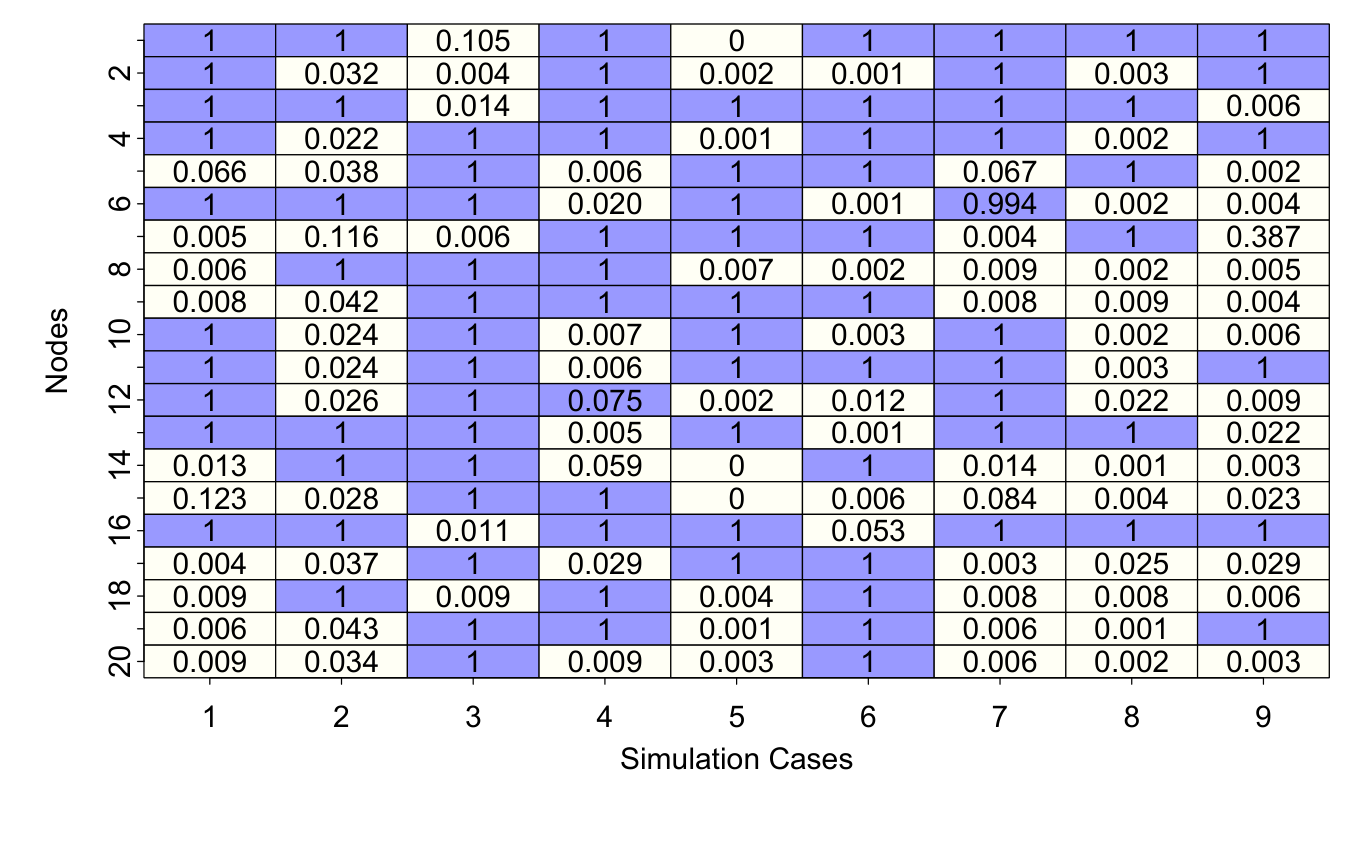
Figure 1 shows a matrix whose rows correspond to different cases in Simulation 1 and columns correspond to the nodes of the network. The dark and clear cells correspond to the truly active and inactive nodes, respectively. The posterior probability of the th node being detected as active, i.e., has been overlaid for all in all simulation cases. The plot suggests overwhelmingly accurate detection of nodes influencing the response. We provide similar plots on node detection in Figure 2 for various cases in Simulation 2 and Simulation 3. Both figures show good detection of active nodes both in Simulations 2 and 3 with very few false positives. We emphasize the fact that BNR is designed to detect important nodes while BLasso, HS or Lasso (or any other ordinary high dimensional regression technique) do not allow node selection in the present context. We have also investigated in detail the nodes selected by Relión et al., 2017 and it is found to perform sub-optimally. For example, in Case -1 of Simulation 1, out of nodes, the number of false positives is .
Estimating the network coefficient
Another important aspect of the parametric inference lies in the performance in terms of estimating the network predictor coefficients. Tables 4, 5, 6 present the MSE of all the competitors in Simulations 1, 2 and 3 respectively. Given that both the fitted network regression coefficient and the true coefficient are symmetric, the MSE for any competitor is calculated in each dataset as , where is the point estimate of , is the true value of the coefficient, and is the number of elements in the upper triangular portions of the matrices and . For Bayesian models (such as the proposed model), is taken to be the posterior mean of .
Table 4 shows that the proposed Bayesian network regression (BNR) outperforms all its Bayesian and frequentist competitors in all cases of Simulation 1. In cases 1-7 when the sparsity parameter is low to moderate, we perform overwhelmingly better than all the competitors. While BNR is expected to perform much better than BLasso, Horseshoe and Lasso due to incorporation of network information, it is important to note that the carefully chosen global-local shrinkage prior with a well formulated hierarchical mean structure seems to possess more detection and estimation power than Relión et al., 2017. When the sparsity parameter in Simulation 1 is high (cases 8-9), our simulation scheme sets an overwhelming proportion of ’s to zero. As a result, BNR only slightly outperforms Horseshoe and BLasso. Again, Relión et al., 2017 does not seem to be competitive, not only against BNR, but also against Horseshoe.
For Simulations 2 and 3, tables 5 and 6 demonstrate that when node sparsity is higher (i.e. when more edge coefficients are set to zero in the data generation procedure), BNR performs very similar to Horseshoe. This might be due to the fact that high degree of sparsity in the edge coefficients in the truth is conducive for ordinary high dimensional regression which treats edges as coefficients. As node sparsity decreases so that more and more edge coefficients are nonzero in the truth and the network structure in the predictors dominates, BNR tends to show more and more advantage in terms of estimating the network coefficient .
Inference on the effective dimensionality
Next, the attention turns to inferring on the posterior expected value of the effective dimensionality of . Figure 3 presents posterior probabilities of effective dimensionality in all cases in Simulation 1. The filled bullets indicate the true value of the effective dimensionality. All 9 figures indicate that the true dimensionality of the latent variable is effectively captured by the models. Variation in the sparsity or discrepancy between and seems to impact the performance very negligibly. Only in cases 8 and 9, in presence of less network information, there appears to be greater uncertainty in the posterior distribution of . We also investigate similar figures for Simulations 2 and 3 (see Figures 4 and 5), though in the absence of any ground truth on effective dimensionality, they are less interpretable.
| MSE | ||||||||
| Cases | Sparsity | BNR | Lasso | Relión(2017) | BLasso | Horseshoe | ||
| Case - 1 | 2 | 2 | 0.5 | 0.009 | 0.438 | 0.524 | 0.472 | 0.395 |
| Case - 2 | 2 | 3 | 0.6 | 0.007 | 0.660 | 0.929 | 0.863 | 0.012 |
| Case - 3 | 2 | 5 | 0.3 | 0.006 | 1.295 | 1.117 | 1.060 | 1.070 |
| Case - 4 | 2 | 5 | 0.4 | 0.006 | 0.371 | 0.493 | 0.699 | 0.298 |
| Case - 5 | 3 | 5 | 0.5 | 0.009 | 1.344 | 1.629 | 1.638 | 1.381 |
| Case - 6 | 4 | 5 | 0.4 | 0.006 | 3.054 | 2.601 | 2.680 | 3.284 |
| Case - 7 | 2 | 4 | 0.5 | 0.009 | 0.438 | 0.524 | 0.472 | 0.395 |
| Case - 8 | 2 | 4 | 0.7 | 0.005 | 0.015 | 0.251 | 0.007 | 0.008 |
| Case - 9 | 3 | 5 | 0.7 | 0.004 | 0.029 | 0.071 | 0.019 | 0.007 |
| MSE | ||||||||
| Cases | Sparsity | BNR | Lasso | Relión(2017) | BLasso | Horseshoe | ||
| Case - 1 | 3 | 5 | 0.7 | 0.011 | 0.013 | 0.036 | 0.010 | 0.008 |
| Case - 2 | 3 | 5 | 0.2 | 0.629 | 0.843 | 0.859 | 0.836 | 0.948 |
| MSE | |||||||||
| Cases | Node | Edge | BNR | Lasso | Relión(2017) | BLasso | Horseshoe | ||
| Sparsity | Sparsity | ||||||||
| Case - 1 | 3 | 5 | 0.7 | 0.5 | 0.004 | 0.006 | 0.017 | 0.004 | 0.003 |
| Case - 2 | 3 | 5 | 0.2 | 0.5 | 0.457 | 0.636 | 0.617 | 0.659 | 0.629 |
3.3 Predictive Inference
For the purpose of assessing predictive inference of the competitors, samples are generated from (7). We compare the predictive ability of competitors based on the point prediction and characterization of predictive uncertainties. To assess point prediction, we employ the mean squared prediction error (MSPE) which is obtained as the average squared distance between the point prediction and the true responses for all the competitors. As measures of predictive uncertainty, we provide coverage and length of predictive intervals. For frequentist competitors, predictive intervals are obtained by using predictive point estimates plus and minus times standard errors. Figure 6 provides all three measures for all competitors in the cases for Simulation 1.
It is quite evident from Figure 6(a) that BNR outperforms other competitors in terms of point prediction. Among the competitors, Horseshoe does a reasonably good job in cases with a higher degree of sparsity. Note that the data generation procedure in Simulation 1 ensures that the elements in the edge coefficient matrix take reasonably large positive and negative values. Additionally, an overwhelming number of edge coefficients is set to zero. Clearly, with a small sample size, all local and global parameters for the ordinary vector shrinkage priors are shrunk to zero to provide a good estimation of zero coefficients. While doing so, they miss out on estimating coefficients which significantly deviate from zero. Thus, the ordinary vector shrinkage priors do a relatively poor job in terms of point prediction. Lasso also fails to provide satisfactory performance for similar reasons. On the other hand, all models provide close to nominal coverage. However, the predictive intervals associated with BNR are much narrower than those of other competitors.
The predictive performance for Simulations 2 and 3 is given in Tables 7 and 8 respectively. Since the data generation schemes in Simulations 2 and 3 do not incorporate network structure, the performance of BNR is comparable to that of its competitors in the high sparsity case. On the other hand, in presence of low node sparsity, the performance of Lasso, BLasso and Horseshoe deteriorate, and BNR turns out to be the best performer.
| MSPE | ||||||||
| Cases | Sparsity | BNR | Lasso | Relión(2017) | BLasso | Horseshoe | ||
| Case - 1 | 3 | 5 | 0.7 | 0.079 | 0.100 | 0.371 | 0.076 | 0.061 |
| Case - 2 | 3 | 5 | 0.2 | 0.432 | 0.726 | 0.859 | 0.629 | 0.725 |
| Coverage of 95% PI | ||||||||
| Case - 1 | 3 | 5 | 0.7 | 1.00 | 1.00 | 0.867 | 1.00 | 0.967 |
| Case - 2 | 3 | 5 | 0.2 | 0.94 | 0.73 | 0.56 | 0.96 | 0.87 |
| Length of 95% PI | ||||||||
| Case - 1 | 3 | 5 | 0.7 | 8.97 | 18.70 | 10.23 | 8.25 | 6.40 |
| Case - 2 | 3 | 5 | 0.2 | 42.18 | 32.81 | 23.54 | 45.69 | 42.91 |
| MSPE | |||||||||
| Cases | Node | Edge | BNR | Lasso | Relión(2017) | BLasso | Horseshoe | ||
| Sparsity | Sparsity | ||||||||
| Case - 1 | 3 | 5 | 0.7 | 0.5 | 0.119 | 0.151 | 0.425 | 0.125 | 0.096 |
| Case - 2 | 3 | 5 | 0.2 | 0.5 | 0.451 | 0.549 | 0.699 | 0.692 | 0.566 |
| Coverage of 95% PI | |||||||||
| Case - 1 | 3 | 5 | 0.7 | 0.5 | 0.93 | 1.00 | 0.86 | 0.96 | 0.96 |
| Case - 2 | 3 | 5 | 0.2 | 0.5 | 1.00 | 0.83 | 0.70 | 1.00 | 1.00 |
| Length of 95% PI | |||||||||
| Case - 1 | 3 | 5 | 0.7 | 0.5 | 6.18 | 14.19 | 8.35 | 6.44 | 5.91 |
| Case - 2 | 3 | 5 | 0.2 | 0.5 | 41.69 | 27.98 | 17.84 | 51.70 | 49.12 |
4 Application to Human Brain Network Data
This section illustrates the inferential and predictive ability of Bayesian network regression in the context of a diffusion weighted magnetic resonance imaging (DWI) dataset. Along with the brain network data, the dataset of interest contains a measure of creativity for several subjects, known as the Composite Creativity Index (CCI). The scientific goal in this setting pertains to understanding the relationship between brain connectivity and the composite creativity index (CCI). In particular, we are interested in predicting the CCI of a subject from his/her brain network, and to identify brain regions (nodes in the brain network) that are involved with creativity, as well as significant connections between different brain regions.
Human creativity has been at the crux of the evolution of the human civilization, and has been the topic of research in several disciplines including neuroscience. Though creativity can be defined in numerous ways, one could envision a creative idea as one that is unusual as well as effective in a given social context (Flaherty, 2005). Neuroscientists generally concur that a coalescence of several cognitive processes determines the creative process, which often involves a divergence of ideas to conceivable solutions for a given problem. To measure the creativity of an individual, Jung et al., 2010 propose the CCI, which is formulated by linking measures of divergent thinking and creative achievement to cortical thickness of young (23.7 4.2 years), healthy subjects. Three independent judges grade the creative products of a subject from which the “composite creativity index” (CCI) is derived. CCI serves as the response in our study.
Along with CCI measurements, brain network information for subjects is gathered using diffusion weighted magnetic resonance imaging (DWI). DWI is an imaging technique that enables measurement of the restricted diffusion of water in tissue in order to produce neural tract images. The brain imaging data we use has been pre-processed using the NDMG pre-processing pipeline (Kiar et al., 2016; Kiar et al., 2017a; Kiar et al., 2017b). In the context of DWI, the human brain is divided according to the Desikan atlas (Desikan et al., 2006) that identifies 34 cortical regions of interest (ROIs) both in the left and right hemispheres of the human brain, implying 68 cortical ROIs in all. A ‘brain network’ for each subject is represented by a symmetric adjacency matrix whose rows and columns correspond to different ROIs and entries correspond to estimates of the number of ‘fibers’ connecting pairs of brain regions. Thus, for each individual, representing the brain network, is a weighted adjacency matrix of dimension , with the th off-diagonal entry in the adjacency matrix being the estimated number of fibers connecting the th and the th brain regions. Figure 7 shows maps of the brain network for two representative individuals in the sample. Each cell of the adjacency matrix is standardized by subtracting the mean and dividing by the standard deviation with respect to all samples. CCI is also standardized in a similar fashion. Now we fit our proposed model with standardized CCI as the response and the standardized adjacency matrix as the network predictor. We use identical prior distributions for all the parameters as in the simulation studies.
The MCMC chain is run for iterations, with the first iterations discarded as burn-in. Convergence is assessed by comparing different simulated sequences of representative parameters started at different initial values (Gelman et al., 2014). All inference is based on the remaining post burn-in iterates appropriately thinned. Moreover, we monitor the auto-correlation plots and effective sample sizes of the iterates.
4.1 Findings from BNR
We focus on identifying influential ROIs in the brain network using the node selection strategy described in the simulation studies. For the purpose of this data analysis, the Bayesian network regression model is fitted with which is found to be sufficient for this study. Recall that the th node is identified as active if exceeds . This criteria, when applied to the real data discussed above, identifies ROIs out of as active. Of these ROIs, belong to the left portion of the brain (or the left hemisphere) and belong to the right hemisphere. The effective dimension of the model a-posteriori is . Table 10 shows the brain ROIs in the Desikan atlas detected as being actively associated with the CCI.
A large number of the active nodes detected by our method are part of the frontal () and temporal () cortices in both hemispheres. The frontal cortex has been scientifically associated with divergent thinking and problem solving ability, in addition to motor function, spontaneity, memory, language, initiation, judgement, impulse control and social behavior (Stuss et al., 1985). Some of the other functions directly related to the frontal cortex seem to be “behavioral spontaneity,” interpreting environmental feedback and risk taking (Razumnikova, 2007; Miller and Milner, 1985 ; Kolb and Milner, 1981). On the other hand, Finkelstein et al., 1991 report de novo artistic expression to be associated with the temporal and frontal regions. Our method also finds a strong relationship between creativity and the right parahippocampal gyrus and right inferior parietal lobule, regions found to be involved with creativity by a few earlier scientific studies, see e.g., Chavez et al., 2004.
As a reference point to our analysis, we compare our findings with Jung et al., 2010, where a regression model is used to understand the relationship between CCI and ROI-specific measures to account for the relationship between creativity and different brain regions. Our analysis finds a number of overlaps with the regions that Jung et al., 2010 identify as significantly associated with the creativity process, namely the middle frontal gyrus, the left cingulate cortex, the left orbitofrontal region, the left lingual region, the right fusiform, the left cuneus, the right superior parietal lobule, the inferior parietal, the superior parietal lobules and the right posterior singulate regions. Although there is significant intersection between the findings of Jung et al., 2010 and our method, there are a few regions that we detect as active and they do not, and vice versa. For example, our model detects the precuneus and the supramarginal regions in both the hemispheres to be significantly related to CCI, while Jung et al., 2010 do not. On the other hand, they identify the right angular region to be significant while we do not. We also implement the method of Relión et al., 2017 on our dataset, and find that it identifies out of ROIs as active. The regions that are found to inactive are the frontalpole, temporalpole and the transversetemporal regions in the right hemisphere.
Along with influential ROIs, we are interested in identifying the statistically significant edges or connections between the ROIs. We consider the edge between two ROIs and to have a statistically significant impact on CCI if the credible interval of the posterior distribution of its corresponding coefficient does not contain . Under this measure, our model identifies significant ’s. Figure 8 plots significant inter-connections detected among brain regions of interest (ROIs), where the brain can be viewed from different angles. Red dots show the active ROIs and blue lines show significant connections between them. Figure 9 plots these influential interconnections, where a white cell represents an edge predictive of the response with the corresponding row ROI and column ROI. Since this is an undirected network, the matrix is symmetric and we only show connections in the upper triangular region.
Finally, our interest turns to the predictive ability of the Bayesian network regression model. To this end, Table 9 reports the mean squared prediction error (MSPE) between observed and predicted responses, length and coverage of 95% predictive intervals. Here, the average is computed over cross-validated folds. As reference, we also present MSPE, length and coverage values for Lasso, BLasso and Relión et al., 2017. Our approach models correlation across coefficients sparsely, which seems to improve the prediction vis-a-vis Lasso and BLasso. The table clearly shows excellent point prediction of our proposed approach even under small sample size and low signal to noise ratio. Additionally, all competitors provide close to nominal coverage, with BNR yielding slightly less than nominal coverage, and the other competitors yielding slightly more, but with much wider credible intervals.
| BNR | Lasso | BLasso | Relión(2017) | |
| MSPE | 0.69 | 0.98 | 1.84 | 0.98 |
| Coverage of 95% PI | 0.93 | 0.97 | 0.97 | 0.97 |
| Length of 95% PI | 2.72 | 3.88 | 3.40 | 3.89 |

| Left Hemisphere Lobes | |||||
| Temporal | Cingulate | Frontal | Occipital | Parietal | Insula |
| inferior temporal gyrus | isthmus cingulate cortex | lateral orbitofrontal | cuneus | precuneus | insula |
| middle temporal gyrus | paracentral | lateral occipital gyrus | superior parietal lobule | ||
| pars opercularis | lingual | supramarginal gyrus | |||
| precentral | |||||
| rostral middle frontal gyrus | |||||
| frontal pole | |||||
| Right Hemisphere Lobes | |||||
| Temporal | Cingulate | Frontal | Occipital | Parietal | Insula |
| bank of the superior temporal sulcus | caudal anterior cingulate | medial orbitofrontal | lingual | inferior parietal lobule | insula |
| fusiform | isthmus cingulate cortex | pars orbitalis | precuneus | ||
| middle temporal gyrus | posterior cingulate cortex | pars triangularis | superior parietal lobule | ||
| parahippocampal | rostral anterior cingulate cortex | rostral middle frontal gyrus | supramarginal gyrus | ||
| superior temporal gyrus | |||||
| transverse temporal | |||||

5 Conclusion and Future Work
This article proposes a novel Bayesian framework to address a regression problem with a continuous response and network-valued predictors, respecting the underlying network structure. Our contribution lies in carefully constructing a novel class of network shrinkage priors corresponding to the network predictor which accounts for the correlation in the regression coefficients that is expected from the relational nature of the predictor. Empirical results from simulation studies show that our method is superior to popular alternatives in situations where the regression coefficients have a network structure, and very competitive in other circumstances, both in terms of inference as well as prediction. Our framework is employed to analyze a brain connectome dataset on composite creativity index along with the brain network of multiple individuals. It is able to identify important regions in the brain and important brain connectivity patterns which have profound influence on the creativity of a person.
A number of future directions emerge from this work. First, our framework finds natural extension to regression problems with a binary response and any network predictor, whether binary or weighted. Such a framework would be useful in various classification problems involving network predictors, e.g., in classifying diseased patients from normal people in neuroimaging studies. Another important direction appears to be the development of a regression framework with the network as the response regressed on a few scalar/vector predictors. Some of these constitute our current work.
Appendix A
This section provides details of posterior computation for all the parameters in the Bayesian network regression with a continuous response.
Let be of dimension , where . Assume and is an matrix. Further, assume , and . Thus, with data points, the hierarchical model with the Bayesian Network Lasso prior can be written as
The hierarchical model specified above leads to straightforward Gibbs sampling with full conditionals obtained as following:
- •
- •
, where and
- •
- •
, where GIG denotes the generalized inverse Gaussian distribution.
- •
- •
, where , and
- •
- •
.
- •
.
- •
, where . Here
, , , , for . - •
, for .
Appendix B
This section shows the posterior propriety of the parameters in the BNR model. Without loss of generality, we set while proving the posterior propriety. To begin with, we state a number of useful lemmas.
Preliminary Results
Lemma 5.1
If is an non-negative definite matrix, then .
The eigenvalues of are given by , where are eigenvalues of . Since is non-negative definite, . The result follows from the fact that is the product of eigenvalues.
Lemma 5.2
Let be an diagonal matrix with diagonal entries all greater than . Suppose is an matrix with the largest eigenvalue of given by . Then , where implies is a positive definite matrix.
Since , . Consider the spectral decomposition of the matrix . Let the eigen-decomposition of , where is the matrix of eigenvectors and is a diagonal matrix with diagonal entries . Since each , . Thus, . Hence .
Lemma 5.3
Suppose is an vector and is an symmetric positive definite matrix. Let be another positive definite matrix such that (where implies is non-negative definite). Then .
implies . Thus all eigenvalues of are greater than or equal to 1. Since commuting the product of two matrices does not change the eigenvalues, has all eigenvalues greater than or equal to 1. Thus , which implies . Then .
Main Result
Note that the posterior distribution of the parameters is given by
Integrating over
Further integrating over yields,
The prior specifications on enable it to be bounded within a finite interval of (0,1). Thus in showing the posterior propriety of parameters with unbounded range, it is enough to treat as constant. We treat it as fixed henceforth.
Note that each , hence marginalizing out gives
Integrating over , we obtain,
Next, we integrate w.r.t. to obtain
| (10) |
(10) is a discrete sum of terms with different combinations of . The sum integrated out over all the parameters is finite if the individual summands are finite when integrated out w.r.t all parameters.
Denote a representative summand by , where
| (11) |
Note the fact that is a diagonal matrix with all positive diagonal entries. Thus is non-negative definite and by using Lemma 5.2
where implies is a non-negative definite matrix and is the largest eigenvalue of . Using Lemma 5.3, the above inequality implies
Let
| (12) |
With little algebra it can be shown that
Therefore, the integral of (10) w.r.t. all parameters is finite if and only if
Henceforth, we will proceed to show that this integral is finite.
With little algebra, we have that
Hence,
Define . Then
| (13) |
Now,
Note that
where the first inequality follows from the fact that for all . The second inequality is a direct application of the Cauchy-Schwarz inequality. By the ratio test of integrals, this integral is finite if is finite. Now use the fact that for any to argue that is finite.
Similarly,
where is the minimum eigenvalue of . The last inequality follows from the fact that
. is finite if and only if , by ratio test of integrals. Since the latter integral is finite, .
Now consider the expression . It is easy to see that is a bounded set, so that the bounded function
achieves the maximum value at . Thus,
where the last step follows from earlier discussions.
References
- Armagan et al. (2013) Armagan, A., Dunson, D. B., and Lee, J. (2013). Generalized double Pareto shrinkage. Statistica Sinica, 23(1), 119–143.
- Bullmore and Sporns (2009) Bullmore, E. and Sporns, O. (2009). Complex brain networks: Graph theoretical analysis of structural and functional systems. Nature Reviews. Neuroscience, 10(3), 186–198.
- Carvalho et al. (2010) Carvalho, C. M., Polson, N. G., and Scott, J. G. (2010). The horseshoe estimator for sparse signals. Biometrika, 97(2), 465–480.
- Chatterjee and Lahiri (2010) Chatterjee, A. and Lahiri, S. (2010). Asymptotic properties of the residual bootstrap for lasso estimators. Proceedings of the American Mathematical Society, 138(12), 4497–4509.
- Chatterjee and Lahiri (2011) Chatterjee, A. and Lahiri, S. N. (2011). Bootstrapping lasso estimators. Journal of the American Statistical Association, 106(494), 608–625.
- Chavez et al. (2004) Chavez, R., Graff-Guerrero, A., Garcia-Reyna, J., Vaugier, V., and Cruz-Fuentes, C. (2004). Neurobiology of creativity: Preliminary results from a brain activation study. Salud Mental, 27(3), 38–46.
- Christakis and Fowler (2007) Christakis, N. A. and Fowler, J. H. (2007). The spread of obesity in a large social network over 32 years. n engl j med, 2007(357), 370–379.
- Craddock et al. (2009) Craddock, R. C., Holtzheimer, P. E., Hu, X. P., and Mayberg, H. S. (2009). Disease state prediction from resting state functional connectivity. Magnetic Resonance in Medicine, 62(6), 1619–1628.
- De la Haye et al. (2010) De la Haye, K., Robins, G., Mohr, P., and Wilson, C. (2010). Obesity-related behaviors in adolescent friendship networks. Social Networks, 32(3), 161–167.
- Desikan et al. (2006) Desikan, R. S., Ségonne, F., Fischl, B., Quinn, B. T., Dickerson, B. C., Blacker, D., Buckner, R. L., Dale, A. M., Maguire, R. P., Hyman, B. T., et al. (2006). An automated labeling system for subdividing the human cerebral cortex on MRI scans into gyral based regions of interest. Neuroimage, 31(3), 968–980.
- Doreian (2001) Doreian, P. (2001). Causality in social network analysis. Sociological Methods & Research, 30(1), 81–114.
- Durante et al. (2017) Durante, D., Dunson, D. B., et al. (2017). Bayesian inference and testing of group differences in brain networks. Bayesian Analysis.
- Erdos and Rényi (1960) Erdos, P. and Rényi, A. (1960). On the evolution of random graphs. Publication of the Mathematical Institute of the Hungarian Academy of Sciences, 5(1), 17–60.
- Finkelstein et al. (1991) Finkelstein, Y., Vardi, J., and Hod, I. (1991). Impulsive artistic creativity as a presentation of transient cognitive alterations. Behavioral Medicine, 17(2), 91–94.
- Flaherty (2005) Flaherty, A. W. (2005). Frontotemporal and dopaminergic control of idea generation and creative drive. Journal of Comparative Neurology, 493(1), 147–153.
- Fosdick and Hoff (2015) Fosdick, B. K. and Hoff, P. D. (2015). Testing and modeling dependencies between a network and nodal attributes. Journal of the American Statistical Association, 110(511), 1047–1056.
- Fowler and Christakis (2008) Fowler, J. H. and Christakis, N. A. (2008). Dynamic spread of happiness in a large social network: longitudinal analysis over 20 years in the framingham heart study. British Medical Journal, 337, a2338.
- Frank and Strauss (1986) Frank, O. and Strauss, D. (1986). Markov graphs. Journal of the American Statistical Association, 81(395), 832–842.
- Friedman et al. (2010) Friedman, J., Hastie, T., and Tibshirani, R. (2010). Regularization paths for generalized linear models via coordinate descent. Journal of Statistical Software, 33(1), 1–22.
- Gelman et al. (2014) Gelman, A., Carlin, J. B., Stern, H. S., Dunson, D. B., Vehtari, A., and Rubin, D. B. (2014). Bayesian data analysis, volume 2. CRC press Boca Raton, FL.
- Gramacy and Gramacy (2013) Gramacy, R. B. and Gramacy, M. R. B. (2013). R package monomvn.
- Guhaniyogi and Rodriguez (2017) Guhaniyogi, R. and Rodriguez, A. (2017). Joint modeling of longitudinal relational data and exogenous variables. https://www.soe.ucsc.edu/sites/default/files/technical-reports/UCSC-SOE-17-17.pdf.
- Guhaniyogi et al. (2017) Guhaniyogi, R., Qamar, S., and Dunson, D. B. (2017). Bayesian tensor regression. Journal of Machine Learning Research, 18(79), 1–31.
- Hoff (2005) Hoff, P. D. (2005). Bilinear mixed-effects models for dyadic data. Journal of the American Statistical Association, 100(469), 286–295.
- Hoff (2009) Hoff, P. D. (2009). A hierarchical eigenmodel for pooled covariance estimation. Journal of the Royal Statistical Society: Series B (Statistical Methodology), 71(5), 971–992.
- Hoff et al. (2002) Hoff, P. D., Raftery, A. E., and Handcock, M. S. (2002). Latent space approaches to social network analysis. Journal of the American Statistical Association, 97(460), 1090–1098.
- Ishwaran and Rao (2005) Ishwaran, H. and Rao, J. S. (2005). Spike and slab variable selection: Frequentist and Bayesian strategies. Annals of Statistics, 33(2), 730–773.
- Jung et al. (2010) Jung, R. E., Segall, J. M., Jeremy Bockholt, H., Flores, R. A., Smith, S. M., Chavez, R. S., and Haier, R. J. (2010). Neuroanatomy of creativity. Human Brain Mapping, 31(3), 398–409.
- Kiar et al. (2016) Kiar, G., Gray Roncal, W., Mhembere, D., Bridgeford, E., Burns, R., and Vogelstein, J. (2016). ndmg: Neurodata’s MRI graphs pipeline.
- Kiar et al. (2017a) Kiar, G., Gorgolewski, K., and Kleissas, D. (2017a). Example use case of sic with the ndmg pipeline (sic: ndmg). GigaScience Database.
- Kiar et al. (2017b) Kiar, G., Gorgolewski, K. J., Kleissas, D., Roncal, W. G., Litt, B., Wandell, B., Poldrack, R. A., Wiener, M., Vogelstein, R. J., Burns, R., et al. (2017b). Science in the cloud (sic): A use case in MRI connectomics. Giga Science, 6(5), 1–10.
- Kolb and Milner (1981) Kolb, B. and Milner, B. (1981). Performance of complex arm and facial movements after focal brain lesions. Neuropsychologia, 19(4), 491–503.
- Kyung et al. (2010) Kyung, M., Gill, J., Ghosh, M., Casella, G., et al. (2010). Penalized regression, standard errors, and bayesian lassos. Bayesian Analysis, 5(2), 369–411.
- Lin (2010) Lin, X. (2010). Identifying peer effects in student academic achievement by spatial autoregressive models with group unobservables. Journal of Labor Economics, 28(4), 825–860.
- Miller and Milner (1985) Miller, L. and Milner, B. (1985). Cognitive risk-taking after frontal or temporal lobectomy-II. The synthesis of phonemic and semantic information. Neuropsychologia, 23(3), 371–379.
- Niezink and Snijders (2016) Niezink, N. M. K. and Snijders, T. A. B. (2016). Co-evolution of social networks and continuous actor attributes.
- Nowicki and Snijders (2001) Nowicki, K. and Snijders, T. A. B. (2001). Estimation and prediction for stochastic block structures. Journal of the American Statistical Association, 96(455), 1077–1087.
- Park and Casella (2008) Park, T. and Casella, G. (2008). The Bayesian lasso. Journal of the American Statistical Association, 103(482), 681–686.
- Polson and Scott (2010) Polson, N. G. and Scott, J. G. (2010). Shrink globally, act locally: Sparse bayesian regularization and prediction. Bayesian Statistics, 9, 501–538.
- Razumnikova (2007) Razumnikova, O. M. (2007). Creativity related cortex activity in the remote associates task. Brain Research Bulletin, 73(1), 96–102.
- Relión et al. (2017) Relión, J. D. A., Kessler, D., Levina, E., and Taylor, S. F. (2017). Network classification with applications to brain connectomics. arXiv preprint arXiv:1701.08140.
- Richiardi et al. (2011) Richiardi, J., Eryilmaz, H., Schwartz, S., Vuilleumier, P., and Van De Ville, D. (2011). Decoding brain states from fMRI connectivity graphs. Neuroimage, 56(2), 616–626.
- Shalizi and Thomas (2011) Shalizi, C. R. and Thomas, A. C. (2011). Homophily and contagion are generically confounded in observational social network studies. Sociological methods & research, 40(2), 211–239.
- Shoham et al. (2015) Shoham, D. A., Hammond, R., Rahmandad, H., Wang, Y., and Hovmand, P. (2015). Modeling social norms and social influence in obesity. Current Epidemiology Reports, 2(1), 71–79.
- Stuss et al. (1985) Stuss, D., Ely, P., Hugenholtz, H., Richard, M., LaRochelle, S., Poirier, C., and Bell, I. (1985). Subtle neuropsychological deficits in patients with good recovery after closed head injury. Neurosurgery, 17(1), 41–47.
- Tibshirani (1996) Tibshirani, R. (1996). Regression shrinkage and selection via the Lasso. Journal of the Royal Statistical Society. Series B (Methodological), 58(1), 267–288.
- Watts and Dodds (2009) Watts, D. J. and Dodds, P. (2009). Threshold models of social influence. The Oxford Handbook of Analytical Sociology, pages 475–497.
- Zhou et al. (2013) Zhou, H., Li, L., and Zhu, H. (2013). Tensor regression with applications in neuroimaging data analysis. Journal of the American Statistical Association, 108(502), 540–552.