Numerical evaluation of inflationary 3-point functions on curved field space
– with the transport method & CppTransport
Abstract
We extend the public CppTransport code to calculate the statistical properties of fluctuations in multiple-field inflationary models with curved field space. Our implementation accounts for all physical effects at tree-level in the ‘in–in’ diagrammatic expansion. This includes particle production due to time-varying masses, but excludes scenarios where the curvature perturbation is generated by averaging over the decay of more than one particle. We test our implementation by comparing results in Cartesian and polar field-space coordinates, showing excellent numerical agreement and only minor degradation in compute time. We compare our results with the PyTransport 2.0 code, which uses the same computational approach but a different numerical implementation, finding good agreement. Finally, we use our tools to study a class of gelaton-like models which could produce an enhanced non-Gaussian signal on equilateral configurations of the Fourier bispectrum. We show this is difficult to achieve using hyperbolic field-space manifolds and simple inflationary potentials.
1 Introduction
Inflation [1, 2, 3] has become established as a preferred framework in which to describe the early universe. In inflation, primordial quantum fluctuations are amplified, giving large-scale variations in energy density that are inherited by later structure. Recent ideas from theories of beyond-the-Standard-Model physics have introduced multiple-field models yielding 2-point statistics consistent with measurement, but which may be theoretically preferable because their field values remain sub-Planckian. In such theories the kinetic term is often non-canonical and is expressed in terms of a kinetic matrix . (We define our notation more carefully below. Here, upper-case Latin indices label the different species of scalar fields, and lower-case indices label spacetime dimensions.) The matrix is real, symmetric, and transforms as a covariant 2-tensor under field redefinitions, so it may be interpreted as a metric. The resulting ‘covariant’ formalism constrains the ways in which can appear in observable quantities and offers a convenient computational framework with the usual advantages of tensor calculus.
Examples in this class include models descending from string theory or supergravity where the kinetic matrix is inherited from a Kähler potential [4, 5]. The -attractor scenario suggested by Kallosh & Linde is of this type [6, 7, 8], including its multiple-field variants [9]. Also, a full description of the interesting Higgs inflation model, including Goldstone modes, requires a noncanonical metric that derives from the Goldstone sigma model [10]. Alternatively, the freedom to choose non-Cartesian coordinates on field space may simply provide a more convenient option, as with the ‘gelaton’ and ‘quasi-single field inflation’ scenarios [11, 12].
Numerical tools.—Whatever the origin of the noncanonical kinetic structure, to constrain such models using modern datasets we require precise numerical predictions. Numerical tools for performing inflationary calculations have existed for some time, but their capabilities have been limited. Ringeval et al. provided the early code FieldInf, which is capable of computing 2-point functions with an arbitrary choice of metric [13, 14, 15], but many other tools restrict to the canonical case . Major examples include ModeCode/MultiModeCode [16, 17, 18, 19], PyFlation [20, 21, 22] and BINGO [23, 24]. ModeCode/MultiModeCode and PyFlation are 2-point function solvers for canonical multiple-field models, and BINGO is a 2- and 3-point function solver for single-field models.
All these are traditional codes that require customization by the user for each model of interest. Recent developments in inflationary perturbation theory [25, 26, 27, 28] have allowed the construction of automated tools [29, 30, 31]. These accept the specification of an inflationary model by its Lagrangian and leverage symbolic algebra methods to produce custom code that solves for the inflationary -point functions. We collectively refer to these as the transport tools (transportmethod.com). The suite contains three tools, all of which apply to multiple-field models:
- •
mTransport [29] is a 2-point function solver implemented in Mathematica. It allows a nontrivial kinetic matrix and is suited to interactive model exploration.
- •
PyTransport [32, 31] is a 2- and 3-point function solver implemented in Python. Version 1 (September 2016) restricted to canonical kinetic terms. Version 2 (September 2017) introduced support for an arbitrary kinetic matrix. Because it is implemented as a Python library it is well-suited to scripting or inclusion in other codes.
- •
CppTransport [33] is a 2- and 3-point function solver implemented in C++. It has built-in functionality to parallelize computations and can postprocess correlation functions to produce inflationary observables. It manages storage of its data products as SQL databases. It is well-suited to larger calculations that benefit from its auto-parallelization or which produce significant data volumes, and performs well with ‘feature’ models containing steps or kinks where its library of sophisticated steppers offers assistance. It is less easy (but still possible) to incorporate within larger codes than PyTransport. The original release 2016.3 restricted to canonical kinetic terms.
In this paper we describe a new release of CppTransport (2018.1) that extends its functionality to nontrivial kinetic matrices. We apply these new tools to a class of gelaton-like scenarios and show that (at least in the scenarios we study) the parameter space available to generate enhanced equilateral correlations is very small. We compare our numerical results with the independent mTransport and PyTransport implementations, finding excellent agreement.11 1 Although the transport tools all use the same computational framework, their numerical implementations vary considerably in detail and therefore this constitutes a nontrivial check on numerical correctness.
Synopsis.—The necessary equations for computation of the inflationary two-point function were given by Mulryne [28] and extended to a non-Euclidean field space by Dias et al. [29]. We have nothing novel to say about this part of the analysis. The extension to three-point correlations was given in Ref. [30], but this was limited to models with canonical kinetic terms.
This paper is divided into three principal parts. First, in §2, we highlight the key modifications required to adapt the analysis of Ref. [30] for a nontrivial field-space metric. A similar discussion has already been given by Ronayne et al. [31]. We briefly review the field-space covariant formulation of inflationary perturbations in §2.1, and use this to derive the covariant cubic Hamiltonian in §2.2. In §2.3 we discuss the computation of initial conditions for each correlation function. We formulate the covariant transport hierarchy in §2.4 and explain how to relate covariant correlation functions to the curvature perturbation in §2.5.
Second, in §3 we present a selection of numerical results. For those wishing to replicate our numerics, we explain how to obtain CppTransport in §3.1. In §§3.2–3.3 we validate our numerical implementation by comparing results computed using polar field-space coordinates with known results in Cartesian coordinates. In §3.4 we apply our method to the ‘gelaton’ model proposed by Tolley & Wyman [11]. In this scenario a light degree of freedom is ‘dressed’ by the interactions of a noncanonical heavy mode, obtaining a subluminal phase velocity and potentially enhanced correlations on equilateral Fourier configurations. Our numerical tools successfully reproduce the features of the scenario, but we show that (at least for the range of potentials we consider) it is difficult to find suitable parameters that allow both sufficient inflation and large enhancement of the equilateral modes. We conclude in §4.
Third, we include a large amount of supplementary information in Appendix A. This includes more detailed computations of the transport hierarchy given in §2, together with a selection of intermediate results not discussed in the main text.
Obtaining CppTransport.—The latest builds of CppTransport and PyTransport are available from the website transportmethod.com. Alternatively, both CppTransport and PyTransport are permanently deposited at zenodo.org; at the time of writing, the current releases are 2018.1 for CppTransport and 2.0 for PyTransport.
Notation.—We use natural units where . The reduced Planck mass is . We use the metric signature . Greek indices label space-time indices, whereas lower-case Roman indices from the middle of the alphabet, , label spatial indices. Upper-case Roman indices label field-space coordinates. We employ a compressed Fourier notation defined in Eq. (4) in which these labels appear in a bold, sans-serif font: . For phase-space coordinates, we use Roman letters from the start of the alphabet, .
2 Differences from the canonical case
To accommodate a non-Euclidean field-space metric we require a covariantization (with respect to the metric ) of the formalism developed in Ref. [30] for the Euclidean case. The advantage of a covariant formalism is that it naturally packages additional terms arising from the metric as Christoffel and Riemann contributions in the same way as spacetime covariance. Its construction entails the replacement of ordinary derivatives by covariant derivatives and contraction of all indices with . However, detailed computations show that Riemann terms also appear, meaning that the resulting formalism is not ‘minimally coupled’ to the field-space curvature. The details of this covariantization were given in Gong & Tanaka [34] and Elliston et al. [35].
Dias et al. [29] applied these ideas to find a covariant formulation of the transport equations for the two-point function. In this section we briefly review this construction and extend it to the three-point function. A more detailed discussion is given in Appendices A.1–A.4.
2.1 Field-covariant formalism
Perturbation series.—In a covariant formalism our aim is to construct correlation functions that transform tensorially under field redefinitions. These are coordinate transformations in field space. Correlation functions of the field perturbations do not have this property, because the coordinates do not themselves transform tensorially (despite the species label ‘’).
A suitable alternative was given by Gong & Tanaka [34], who observed that in a normal neighbourhood of we can associate with the geodesic that connects it to . The geodesic is uniquely determined by its tangent vector at . By construction is field-space covariant and is defined in the unperturbed spacetime. It is therefore a candidate to appear in correlation functions of the form , , …, , each of which will inherit a tensorial transformation law from . See Refs. [34, 35, 29] for further details.
Correlation functions.—After quantization, our intention is to compute 2- and 3-point correlation functions of the Heisenberg-picture fields together with their canonical momenta , where is the covariant time derivative and . As usual, in order to use time-dependent perturbation theory, we split the Hamiltonian into free and interacting parts corresponding to the quadratic and cubic (or higher) terms [30]. Notice that, with this definition, all mass terms are included in the free Hamiltonian. Finally, we define interaction-picture fields and that are related to the Heisenberg-picture fields by a similarity transformation , , where is the unitary operator
| (1) |
and is the anti-time ordering operator that arranges the fields in its argument in order of increasing time. The interacting part of the Hamiltonian is . The notation ‘’ indicates that the integral is to be performed over a contour deformed away from the real axis into the positive complex plane in the distant past, with analytic continuation used to define the integrand. This can be regarded as the theorem of Gell-Mann & Low in the present context [36, 37].
We frequently collect the phase-space coordinates , into a single vector , and likewise for the interaction picture fields . Latin indices , , …, from the early part of the alphabet run over the dimensions of phase space, on which the metric should be taken to have block-diagonal form
| (2) |
The vacuum expectation value of any (possibly composite) Heisenberg-picture operator can be written in terms of , and the interaction picture fields using
| (3) |
where is the vacuum of the free Hamiltonian. We describe Eq. (3) as the ‘in–in’ formula, use it compute all correlation functions of cosmological perturbations in our field-covariant formalism. For further details, see Appendix A.1.1 for the definition of the covariant variable , and Appendix A.2.1 for the definition of correlation functions.
2.2 Hamiltonian
In addition to the change from to , the Hamiltonian acquires new terms generated by derivatives of the metric. The procedure to calculate these follows Maldacena [38, 39, 40]. We minimally couple fields to gravity, allowing a nontrivial kinetic matrix and a potential , and use the ADM decomposition to integrate out the Hamiltonian and momentum constraints. Finally the result is expanded to the desired order in perturbations. The computation to third order in was done by Elliston et al. [35], or see Appendix A.1.4 for further details.
Summation convention.—To write the results, we use a compact notation in which repeated index labels imply both summation over species labels and integration over Fourier wavenumbers. We indicate that this convention is in use by writing the species indices in bold sans-serif. Specifically, such contractions should be interpreted to mean
| (4) |
where, as always, the field metric is used to raise and lower indices. In some manipulations a -function can be produced that changes the sign of a momentum label. We indicate this by placing a bar on each index for which the sign of the momentum should be reversed, eg.,
| (5) |
Second- and third-order kernels.—To third order, the result can be written
| (6) | ||||
where the second-order kernels and are defined as
| (7) | ||||
and the mass-matrix satisfies
| (8) |
Then the third-order kernels , and are given by
| (9a) | ||||
| (9b) | ||||
| (9c) | ||||
and the corresponding ‘species tensors’ are
| (10a) | ||||
| (10b) | ||||
| (10c) | ||||
The brackets surrounding indices in the Riemann terms indicate that the enclosed indices should be symmetrized with weight unity, except for indices between vertical bars which are excluded. Further, note that the tensor should be symmetrized over all three indices with weight unity, and , should be symmetrized over with weight unity. The indices on the momentum labels , , correspond to field-space labels as , and , and should be permuted during symmetrization. The quantity is defined by
| (11) |
From these expressions it is simple to calculate the Hamiltonian using a Legendre transformation. We define the canonical momentum to satisfy
| (12) |
where the variational derivative can be computed using the rule
| (13) |
To compute the Hamiltonian we require the relation which should be regarded as a function of and . Finally, for convenience, we rescale the momentum by a factor , viz. , to obtain the final third-order Hamiltonian,
| (14) | ||||
The second-order terms on the first line and represent the free part of the Hamiltonian , and the third-order terms on the second line represent the interacting part of the Hamiltonian . The new contributions introduced by derivatives of the nontrivial field-space metric are given by the Riemann terms found in the , and tensors.
2.3 Initial conditions
We will require suitable initial conditions for each correlation function on subhorizon scales. To compute these we use Eq. (3) to compute each correlation function at sufficiently early times—normally between four and ten e-folds inside the horizon, although the precise numbers are model-dependent; see Ref. [29]—that all species can be approximated as massless. Such a time can normally be found, provided all masses remain bounded, because the physical wavenumber corresponding to a fixed comoving wavenumber is pushed into the ultraviolet at early times, making each mode kinetically dominated for sufficiently small . The outcome is that we can compute universal initial conditions applicable to any model, no matter what mass spectrum or interactions it contains, provided the computation of its correlation functions begins sufficiently far inside the horizon [29, 30]. For more details see §3 of Ref. [29] and §6 of Ref. [30].
Two-point function.—A suitable initial condition for the covariant equal-time 2-point function was computed by Dias et al. [29], following Elliston et al. [35]. In our notation their results can be written
| (15a) | ||||
| (15b) | ||||
| (15c) | ||||
| (15d) | ||||
where the time-dependent quantities , and appearing on the right-hand sides should be evaluated at the initial time , indicated by the subscript ‘init’ attached to each correlation function.
Eqs. (15a)–(15d) are effectively the same as those found in the canonical case [30] except that the Euclidean kinetic matrix is replaced by the metric . For further details of the computation see Appendix A.3.1.
Three-point function.—Initial conditions for the 3-point functions require the in–in formula (3). The lowest-order nonzero contribution to each correlator is given by
| (16) |
where ‘perms’ indicates a sum over permutations of the pairing between ‘external’ indices and the ‘internal’ indices LMN, ‘c.c.’ indicates the complex conjugate of the preceding term, and contains all the cubic terms found in Eq. (14). For further details we refer to Appendix A.3.2.
To express the results we require some extra notation. First, we divide into ‘fast’ terms, which involve the scale factor and evolve exponentially fast in e-folds, and ‘slow’ terms, which evolve on slow-roll timescales,
| (17) |
The fast term grows rapidly on subhorizon scales and is always relevant when computing initial conditions. In Ref. [30] it was explained that the slow terms can also be relevant in scenarios with enhanced three-body interactions such as a QSFI model.
Second, we introduce the quantities , and . The results for each correlation function are22 2 Eq. (18d) corrects a minor typo in v1 and v2 of the arXiv version of Ref. [30]. This typo was corrected in the arXiv v3.
| (18a) | ||||
| (18b) | ||||
| (18c) | ||||
| (18d) | ||||
All time-dependent quantities on the right-hand side are to be evaluated at the initial time , and the tangent-space indices , , , …, live in the tangent space associated with this time.
Where permutations are specified, they should be carried out only within the bracket in which the instruction to sum over permutations is given. (Notice that these means some momentum factors, such as those multiplying the square-bracket terms in Eqs. (18b) and (18c), are not symmetrized. This is correct because these momentum factors arise from wavefunctions associated with the external fields, and these are not symmetric.) Each permutation should be formed by simultaneous exchange of the species labels , , and their partner momenta , , .
2.4 Covariant transport equations
Next, we require differential equations to evolve each correlation function from its initial value to any time of interest. These equations were derived in the superhorizon limit by Mulryne et al. [25, 26, 35] and later extended to cover the subhorizon era [28, 29].
The procedure to derive these evolution equations matches that of Dias et al. [30]. We begin from the Hamiltonian (14), which can be written in the generic form
| (19) |
The corresponding covariant evolution equation is
| (20) |
where and are phase-space tensors that can be expressed in terms of and [30]. The derivative should be taken to act in phase space with a block-diagonal connexion. For example, acting on contra- and covariant indices this produces
| (21) |
where is the block matrix
| (22) |
In each block represents the species label associated with the phase-space label , and represents the species label associated with .
A similar equation can be found for the fields in the interaction picture. Using Eq. (3) to deduce tree-level expressions for the 2- and 3-point functions in terms of interaction-picture fields, it follows that evolution equations can be derived by direct differentiation and use of the interaction-picture equations of motion to rewrite time derivatives. The results are
| (23a) | ||||
| (23b) | ||||
where we have written the phase-space 2- and 3-point functions as
| (24a) | ||||
| (24b) | ||||
These equations match those in the canonical case except that the time derivative is now covariant and will introduce terms involving the connexion components. A more detailed derivation of these equations can be found in Appendix A.2.2.
For practical calculations we need explicit expressions for the -tensors. They are [30]
| (25a) | ||||
| (25b) | ||||
in which the index labels rows of the top-level matrix. For , the index labels the remaining columns; for , the indices label rows and columns of each submatrix. As above, the field-space labels , , represent the species associated with the phase-space labels , and .
Further details of the calculation, including the Heisenberg equations of motion for and , can be found in Appendix A.2.3.
2.5 Gauge transformation
Although the formalism of covariant correlation functions is computationally convenient, the covariant perturbations and their statistical properties are not directly measurable. The final step is therefore to express correlation functions of measurable quantities such as the curvature perturbation in terms of the covariant correlation functions. This is a covariantization of the gauge transformation from the spatially flat gauge to the uniform density gauge [41, 29, 30].
Using the methods of Ref. [41] we find that the density fluctuation on spatially flat slices can be written in terms of the covariant perturbations ,
| (26) | ||||
where and , respectively, are the first- and second-order perturbations to the lapse. We have neglected spatial gradients that become negligible on superhorizon scales.
Eq. (26) is superficially different to the canonical case due to the final term involving the Riemann tensor. However, the same term appears in the Hamiltonian constraint (see Eq. (85)), and after using this constraint to simplify (26) the result matches the naïve covariantization of the canonical formula [41].
Using the results of Dias et al. [41] to express in terms of , it follows that the curvature perturbation can be written in the form
| (27) |
The coefficient matrices and are given by
| (28a) | |||
| (28b) |
3 Numerical results
We are now able to solve the equations obtained in §2 and use them to compute the observable 2- and 3-point functions of an arbitrary model with user-defined kinetic mixing matrix.
Overview.—In summary, this involves obtaining numerical solutions to the 2- and 3-point function transport equations (23a)–(23b), using the -tensors specified in (25a)–(25b). In turn, these depend on the kinetic matrix and the ‘species tensors’ , , and that specify the Hamiltonian (cf. Eq. (14)). They must be determined for each model from the general formulae (7) and (10a)–(10c). The initial conditions are given by Eqs. (18a)–(18d), provided a suitable initial time can be found at which the massless approximation is valid for all species. These initial conditions also depend on , , , and . Finally, Eqs. (28a) and (28b) are used to construct the correlation functions of .
Each of the transport tools mTransport, CppTransport and PyTransport uses symbolic algebra to automate the calculation of , , and from a specification of the kinetic matrix and the potential . With explicit expressions for each tensor, it is possible to set up the transport equations and compute suitable initial conditions. Additionally, both CppTransport and PyTransport automate the task of finding a suitable initial time at which the massless approximation is valid; in mTransport this currently has to be done by hand, or a suitable initial time estimated.
Notation.—When discussing concrete models we generally use the dimensionless power spectrum , defined in terms of the ordinary power spectrum (see Eq. (163)) using
| (29) |
The analogous quantity for the three-point function is the ‘dimensionless bispectrum’, defined by
| (30) |
We also use the reduced bispectrum, conventionally written , which is defined to satisfy
| (31) |
Notice that this is not the same as the parameter measured by CMB experiments, although in models where the bispectrum is dominantly of the ‘local’ type it is closely related to it.
To specify the configuration of Fourier wavenumbers that characterize the bispectrum we use the parametrization suggested by Fergusson & Shellard [42],
| (32a) | ||||
| (32b) | ||||
| (32c) | ||||
The overall scale of the momentum triangle is measured by its perimeter , and its shape is measured by and . The allowed ranges are and .
By default, CppTransport uses its own ‘internal normalization’ in which a distingished wavenumber is defined to exit the horizon at a chosen time . In this normalization, other wavenumbers are measured relative to by giving the ratios or respectively. This convention means that all wavenumbers quoted in this section are dimensionless. In each case we quote the corresponding value of . Where other horizon exit times are given, these are measured relative to the initial conditions at .
3.1 Obtaining the transport codes
All tools (mTransport, CppTransport and PyTransport) can be downloaded from the website transportmethod.com. At the time of writing the current version of PyTransport is v2.0 and the current version of CppTransport is 2018.1. Alternatively, development versions of CppTransport and PyTransport can be downloaded from their respective GitHub repositories. In this paper we focus on the new features in CppTransport that support an arbitrary metric .
An introduction to CppTransport was given in §8 of Dias et al. [30] and a comprehensive user guide is available on the arXiv [33]. When making use of the new features available in 2018.1 most steps remain the same, with only minor variations:
- •
To use a nontrivial metric it is first necessary to specify that the model is non-canonical by including the directive
lagrangian = nontrivial_metric;in the model block of the input file. Having done so the metric can be specified along with the potential as a list of components surrounded by square brackets [ ]. For example, the metric on a flat two-dimensional field-space in polar coordinates would be written
metric = [ R, R = 1; theta, theta = R^2; ];Off-diagonal elements need be specified only for the upper or lower triangle, and entries that are not given are assumed to be zero. Elements can make use of subexpressions declared elsewhere in the model file.
- •
A suitable set of templates must be chosen for the core and implementation files that use correct index placement and employ the covariantized formulae given in §2. An extra set of templates with these properties is bundled with 2018.1. To use them, the template block of the model file should read
All Riemann terms will be correctly included in the -tensors and initial conditions, and the transport equations will include correct connexion components.
3.2 Cartesian versus polar coordinates
We begin by reproducing results for the gelaton-like scenario [11] studied in Dias et al. [30]. This is an ‘adiabatic-like’ model in which a continuously-turning light field is dressed by the fluctuations of a transverse heavy field, and has similarities to the scenario of quasi-single field inflation [12]. Because the heavy field tracks the minimum of the effective potential, slightly displaced due to the radial motion of the light field, the model behaves as if it has a single collective degree of freedom.
The model is most conveniently expressed in polar field-space coordinates and , and therefore Ref. [30] performed a coordinate transformation to Cartesian fields , to produce a Euclidean kinetic matrix. In this section we study the model in its original polar formulation, finding excellent agreement. The Lagrangian is
| (33) |
where is the heavy field and is the light field. The field-space metric is
| (34) |
In Ref. [30] the potential was chosen so that it represents a circular valley at fixed . The angular velocity was chosen so that a rotation through occurred over approximately 30 e-folds. A suitable choice is
| (35) |
with the parameters , , , and .
Ref. [30] used initial conditions corresponding to
| (36a) | ||||
| (36b) | ||||
In polar coordinates these become
| (37a) | ||||
| (37b) | ||||
The background evolution is plotted in Fig. 1. Inflation lasts for 28 e-folds, and the field evolutions match to high accuracy.
In the left panel of Fig. 2 we plot the dimensionless power spectrum of together with its residual, defined by . The results agree to better than . The right panel gives a similar comparison for the dimensionless bispectrum, showing agreement to better than .
In Fig. 3 we compare the predicted value of the reduced bispectrum . The left-hand panel shows its time evolution for a single Fourier configuration that exits the horizon at 8.0 e-folds. The results agree to within , where the largest residual is given during the rapid evolution of during horizon crossing.
The right panel of Fig. 3 shows the values measured at the end of inflation as a function of wavenumbers that exit the horizon between 17.0 and 24.2 e-folds after the initial conditions are set. Here the residuals are typically at the level with the maximum residual at 0.07%. These are different from the left panel due to the values exiting much later, at a time closer to the end of inflation at 28.0 e-folds where the bispectrum has rapid small-amplitude oscillations.
Despite the vs. plot having larger residuals, these results indicate that the non-canonical transport formalism agrees with its canonical counterpart to within at least when applied to this model.
3.3 Quasi-two-field inflation
Dias et al. [29] introduced a ‘quasi-two-field’ model in which two light scalars drive inflation. One of these fields excites a heavy third field via a noncanonical kinetic coupling, giving rise to oscillatory features in the power spectrum. This is an extension of a simpler two-field model suggested by Achúcarro et al. [43]. Such oscillatory features have been well-studied in the literature [44, 43, 45, 46, 47]. The power spectrum was computed using mTransport by Dias et al. [29], and the bispectrum was computed using PyTransport by Ronayne et al. [31], giving us an opportunity to benchmark CppTransport against the other transport tools. Note that this is not an empty comparison, because although all the transport tools use the same underlying framework they make very different numerical choices in implementation.
The three fields in the model are labelled , and , and the field-space metric is
| (38) |
where is defined to equal [43]
| (39) |
where is the maximum value of , is the value of at the apex of the turn and is the range of during the turn. The potential is
| (40) |
with parameters , , , . The initial conditions are
| (41a) | |||
| (41b) | |||
| (41c) | |||
Two-point function.—In this section, we define the residual between the mTransport and CppTransport power spectrum as
| (42) |
In the left panel of Fig. 4 we plot the residual as a function of time for the -mode that exits the horizon e-folds from the initial time. During the superhorizon phase the agreement is typically at or better, except at a small number of points where the evolution is particularly rapid.
Note that the solutions diverge on subhorizon scales. As explained in Ref. [41], the curvature perturbation does not have a unique definition on subhorizon scales, and the precise value we assign depends which -dependent terms are kept. mTransport uses the ‘local’ form of defined in Ref. [41], whereas CppTransport and PyTransport uses the ‘simple’ form (which agrees with Eqs. (28a)–(28b)). At linear level these are [41]
| (43a) | ||||
| (43b) | ||||
The ‘local’ form mixes and whereas the ‘simple’ form involves only . Correlation functions involving increase on subhorizon scales more rapidly than correlation functions of alone, which accounts for the different time-dependence visible in Fig. 4 on subhorizon scales. The discrepancy is harmless. On superhorizon scales the two forms agree to high accuracy, as they should.
Although this difference means that the correlation functions cannot be compared directly on subhorizon scales, we have verified that the field correlation functions (which are unambiguous) agree to 5 significant figures.
In the right panel of Fig. 4 we plot the residuals as a function of scale for a range of -modes exiting the horizon up to 5.3 e-folds from the pivot scale. The residuals remain below over the whole range. This shows excellent agreement between mTransport and CppTransport despite the rapid oscillations visible in the power spectrum.
Three-point function.—To compare 3-point functions we use the latest version of PyTransport [31]. For each measure of 3-point correlations we define the residual .
In the left-hand panel of Fig. 5 we plot the residual of the dimensionless bispectrum as a function of time for an equilateral configuration where exits the horizon roughly 20 e-folds after the initial time. Our results agree at roughly through most of the evolution, with short-lived excursions to larger values at times of rapid evolution. In the right-hand panel we give an equivalent plot for the reduced bispectrum . We conclude that the variation in numerical results between any two of the transport tools is negligible in comparison with current experimental errors.
The left panel of Fig. 6 shows the residual of the reduced bispectrum as a function of for scales exiting the horizon between 10.9 and 19.9 e-folds after the initial time. Agreement between CppTransport and PyTransport is at the level over almost the entire range of , despite the extremely rapid oscillations visible in the range . In the right panel we show a zoomed-in section highlighting the region of most significant disagreement. The cause of the discrepancy is currently under investigation. This is the only model we have encountered in which our codes show a small disagreement of this kind.
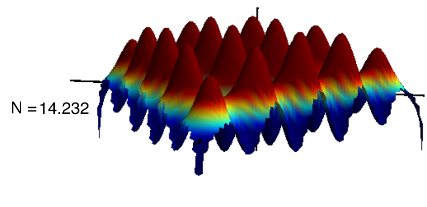
Shape plots.—Up to this point we have focused on the bispectrum amplitude as a function of time or scale, but important information is also encoded in the shape regarding the type of interactions that appear in the Lagrangian. In Fig. 7 we show the dimensionless bispectrum as a function of and at fixed , rescaled to have unit amplitude on the equilateral configuration [42]. We choose so that the wavenumber characterizing this configuration exits the horizon 16.6 e-folds after the initial conditions, and the plots depict the shape given 14.232 e-folds after the initial conditions. In the left panel we show the amplitude as a surface plot with the -height representing the (rescaled) bispectrum amplitude, and in the right panel we give a corresponding contour plot.
At the time given in Fig. 7, the shape shows 15 separate peaks that have evolved from an equilaterally-dominated bispectrum with a single maximum at the equilateral configuration. During the subhorizon phase of inflation, each region of the shape continuously subdivides, generating further peaks. The subdivision continues until horizon-crossing at , after which 8 peaks have formed along each side of the shape plot. The bispectrum shape is briefly re-excited during the turn at e-folds before settling to a constant value until the end of inflation. This behaviour is best seen in our video of the surface plot evolution available on Vimeo.

3.4 The gelaton model
We now apply our tools to a new example: the gelaton model introduced by Tolley & Wyman [11]. In this model a heavy gelaton field, with a mass , is strongly coupled to a light field and dresses its excitations. This causes the light field’s dynamics to be modified. Tolley & Wyman modelled this behaviour using an action with nontrivial kinetic mixing,
| (44) |
Here is the gelaton, is the inflaton, and we can see that the field-space metric is given by:
| (45) |
The function is chosen so that the effective mass of the gelaton is much larger than , ensuring that it remains at the minimum of its effective potential. This is displaced from the minimum of the bare potential due to the kinetic coupling. We label the true minimum , which should be determined by the condition that the field is in static equilibrium,
| (46) |
where is the kinetic energy of . After integrating out from the action (44) it can be shown that the resulting low-energy theory is equivalent to a model [11] in which the action is an arbitrary function of and . Expanding the low-energy action to second order shows that the dressed fluctuations propagate with phase velocity
| (47) |
where is the effective gelaton mass. It is known that models in which the speed of sound is significantly different from unity give enhanced three-point correlations on equilateral configurations [39, 48, 49, 50]. The gelaton model will exhibit such a phenomenology if the speed of sound can be depressed significantly below unity, , while keeping the gelaton mass large, .
DBI potential.—We now specialize to the ‘hyperbolic manifold’ scenario suggested by Tolley & Wyman in which . With this choice, the dynamics of DBI inflation can be replicated by adopting the following potential
| (48) |
where is a free parameter used to adjust the gelaton mass, is the brane tension in the DBI interpretation, and is a potential representing interactions between the brane and other degrees of freedom in the geometry. The gelaton mass is
| (49) |
To fix the model we must specify and . We adopt
| (50a) | ||||
| (50b) | ||||
where , , and . The potential is chosen to keep the expectation value of sub-Planckian. It can be assumed to be representative of any hilltop potential provided does not become too large.
The initial conditions for the two fields are and respectively.
Results.—We perform numerical computations with the full two-field model, to determine whether the low-energy effective description containing only the dressed light fluctuation is an accurate representation of the dynamics. We find very good agreement between our numerical results and the predictions of the low-energy effective theory.
In the left panel of Fig. 8 we plot the evolution of the background fields from their initial values at until the end of inflation at . At early times the evolution of is dominated by its kinetic coupling. The field is driven by the term in . In the right panel we show the evolution of the power spectrum for a single -mode leaving the horizon at . It exhibits smooth decay inside the horizon and asymptotes to a constant value on superhorizon scales, as it should for an effectively single-field model.
In the left panel of Fig. 9 we plot the evolution of the dimensionless bispectrum for an equilateral configuration with fixed corresponding to horizon exit at a time . In the right panel we show the reduced bispectrum evaluated on equilateral configurations as a function of scale, for a range of exiting the horizon between and e-folds after the scale which exits 3.0 e-folds after the initial time. We see that, with this choice of parameters, the enhancement of equilateral configurations is only modest, yielding for a large range of before the end of inflation causes to grow slightly as increases.


In Fig. 10 we plot the shape of the reduced bispectrum for a single -value that exits the horizon 18.9 e-folds after the initial conditions. As before, the left panel shows a three-dimensional surface plot and the right panel shows the corresponding contour plot. Both are evaluated at time , when the time dependence has settled down to become constant. At peak, in agreement with the values plotted in Fig. 9 (for a different value of ), which is still some way from the smallest observable value . The shape plot shows that the detailed structure of the bispectrum is somewhat complicated, although it resembles the equilateral template in its overall structure.
In the next section we will show that an observationally-relevant amplification of the bispectrum is difficult to achieve for a gelaton model of this type, because consistency constraints give very little parameter space to depress the speed of sound.
3.4.1 Gelaton model parameter constraints
The effective single-field description of the gelaton model is applicable only when the gelaton mass is significantly larger than . For smaller masses we must revert to the full two-field description. We now argue that the modest amplitude of seen in Figs. 9 and 10 is a consequence of simultaneously satisfying this and other consistency conditions.
Gelaton mass.—First, we require . With our choice of tension , Eq. (49) shows that
| (51) |
Evidently, if the argument of the exponential term is large then the gelaton mass will be exponentially suppressed. Therefore we suppose , allowing a Taylor expansion of . The leading term is
| (52) |
To estimate the Hubble parameter we assume that the slow-roll approximation applies, making the kinetic terms are sub-dominant to the potential. Under these circumstances a reasonable approximation to will be
| (53) |
where from Eq. (48) has been inserted assuming our choices for and .
Our assumption that the exponential in Eq. (51) is not significantly suppressed makes the term in (53) negligible. Therefore the most significant contribution to will come from the potential . Meanwhile, to prevent higher order terms become relevant we must constrain the negative term to be significantly smaller than the hilltop amplitude . This yields
| (54) |
In this regime the dominant contribution to the Hubble rate will come from the hilltop,
| (55) |
Eqs. (52) and (55) can be used together with the consistency condition to yield a minimum value of the expectation value,
| (56) |
Consistency of Eqs. (54) and (56) yields a constraint on the mass ,
| (57) |
Speed of sound.—Second, to give at least modest suppression of the sound speed we suppose . Eq. (47) then requires
| (58) |
where, as before, we have performed a Taylor expansion in exponentials of . The slow-roll approximation can be used to estimate ,
| (59) |
Combining Eq. (59) and (58) now yields a lower bound for ,
| (60) |
The constraint is the principal obstruction to finding parameter combinations that would yield significant amplification of the equilateral correlations. Most obviously, Eq. (57) creates a tension with the upper bound (57) causing the available parameter window for to be rather narrow. The lower limit scales parametrically with whereas the upper limit scales with , and therefore one strategy to increase the size of the window is to increase . Unfortunately, Eq. (58) shows that increasing will typically force the speed of sound towards unity unless can be changed to compensate. This cannot happen in the slow-roll regime because (59) shows that is independent of .
For example, with the above choices of , and , the window for is . This is so narrow that it is not really possible to have the strong ‘’ inequality satisfied on either side. As we will see below, our choice amply satisfies the upper bound (57) and is sufficient to guarantee , but it violates the lower bound and therefore does not yield a suppressed speed of sound.
The limits on the expectation value (54) and (56) give another constraint. Both limits scale with and therefore the relative size of the window does not change with scaling . Instead, we must rely on changing the parameters or that appear in the denominators of (54) and (56) respectively. We have already seen that is tightly constrained, making the upper limit practically fixed once is prescribed. Also, if is not too close to its lower limit then it will also scale roughly with . Therefore parametrically widening the available window for the expectation value depends on increasing to decrease the lower limit relative to the upper one. Unfortunately must be fairly small in order to keep reasonable small. If the exponential becomes too large then typically grows also, causing inflation to end exponentially quickly. Therefore, in addition to the small range of , there is a very small range of values that satisfy the constraints for a suppressed speed of sound. In our example the range is roughly . This means that it is typically not possible to sustain enhanced three-point correlations for a significant number of e-folds.
We have not succeeded in finding parameter combinations that give a significant enhancement to equilateral correlations while respecting the consistency conditions of the theory. This does not rule out the possibility that the gelaton model can do so, but it would require a different functional form for the potential or the brane tension. We have verified that similar constraints operate for the simplest monomial chaotic models for integer , and that these constraints likewise lead to very narrow windows for and . A modification to the brane tension is possible, but any exotic form would need careful microphysical justification.
Numerical comparison.—In the left panel of Fig. 11 we plot the gelaton mass, , together with the Hubble rate, . We demonstrate that so that it is consistent to integrate out the gelaton. Comparison of our numerical results and the analytic estimates given in this section shows that our approximations for , , and are each accurate to within an order of magnitude. In the right panel we plot the departure of the speed of sound from unity, . This is very small, with approximate value using our parameter choices.
Together, the constraints on the gelaton model with a hilltop potential mean that it is possible to get an inflating solution lasting for approximately 50 e-folds, but only without significant amplification of equilateral non-Gaussianities. A similar conclusion applies if we replace the hilltop potential by a monomial large-field model. This does not rule out the possibility that a different gelaton model could achieve significant enhancement, but the resulting model is likely to more complex than the one considered here.
4 Conclusions
We have applied the transport method to calculate the primordial bispectrum produced by inflationary models containing non-canonical kinetic terms. To do so we leverage the formalism of covariant perturbations suggested by Gong & Tanaka [34] to obtain a covariant Hamiltonian up to third order (§§2.1–2.2). In agreement with other analyses, we show that up to a small number of Riemann terms appearing in , and , the formalism covariantizes naïvely. Moreover, the initial conditions and gauge transformation to also covariantize naïvely provided index positioning is respected (§§2.3–2.5). In §2.4 we demonstrate how to obtain a covariant hierarchy of transport equations.
We have implemented these equations in a new version of the CppTransport tool, which is now capable of handling models with an arbitrary kinetic mixing matrix. At this time, all three transport tools (mTransport, CppTransport and PyTransport) support models of this kind and we can perform a meaningful comparison between them. We find excellent agreement between the different codes (§3.3), with differences typically less than . We also find excellent agreement for the same model written in different field-space coordinates (§3.2) for which differences typically manifest at less than .
In §3.4 we used CppTransport to obtain numerical predictions for a concrete implementation of the gelaton model. We find good agreement between our numerical results (which capture the full dynamics of the two-field model) and the predictions of the single-field effective description in which the gelaton dresses the light fluctuations, giving them a suppressed speed of sound. We find a small boost in the equilateral bispectrum at the level on equilateral configurations. We give an analytic argument that it is not possible to achieve more dramatic enhancements, at least with the potential designed to reproduce the dynamic of the Dirac–Born–Infeld model, without considering more exotic forms for the potential or brane tension.
To summarise, we have extended the automated numerical framework presented by Dias et al. [30] to include more complex models with a non-trivial kinetic term . As before, this allows numerical calculation of all tree-level contributions to the bispectrum and includes physical effects both before and after horizon-crossing. Practically, this means that observable statistics can be found for inflationary models containing a non-trivial kinetic sector, which can include supergravity theories (eg. Refs. [6, 8]) or models motivated by string-theory (eg. Refs. [51, 52]). In future we plan to extend CppTransport to allow sampling over the prior probabilities for initial conditions or Lagrangian parameters, enabling estimates of the important observable parameters such as or in multiple-field models [16, 17, 18, 19].
Acknowledgements.
The work reported in this paper has been supported by the European Research Council under the European Union’s Seventh Framework Agreement (FP7/2007–2013) and ERC Grant Agreement No. 308082. We would like to thank David Mulryne and John Ronayne for helpful conversations.Appendix A Appendix: Detailed calculations
A.1 Perturbed action in curved field space
We begin with an action coupled to scalar fields , minimally coupled to gravity with a self-interaction potential ,
| (61) |
where is the Ricci scalar, and we use Greek indices and upper case Roman indices for the space-time and field-space coordinates respectively. The kinetic mixing matrix is symmetric and positive definite, and can be regarded as a metric on field-space. The case of canonical kinetic terms corresponds to a flat, Euclidean metric.
In this section we simplify calculations by setting the Planck mass to unity, .
A.1.1 Field-covariant perturbations
For a bispectrum calculation we require an expansion in the field perturbations up to third order, where each fluctuation is given by a coordinate displacement . Here, is the background field and is the perturbed field. Unfortunately this expression is not covariant under a change of field coordinates. To obtain a covariant formulation we follow the treatment of Gong & Tanaka [34], who focused on the unique geodesic connected the field-space coordinates of the perturbed and unperturbed fields. We take this geodesic to be labelled by an affine parameter , with normalization adjusted so that at the unperturbed coordinate at at the perturbed coordinate. The initial tangent vector to the geodesic is then defined by
| (62) |
We can then assume parallel transport for our affine parameter and write the geodesic equation as
| (63) |
where denotes a covariant derivative and is a field-space Christoffel symbol. We can then introduce a covariant Taylor expansion of the perturbation, ,
| (64) |
(Note that the appearance of this equation depends on our normalization convention for , but its physical content is independent of it.) Equations (62) & (63) can then be inserted into Eq. (64) to obtain
| (65) |
where ‘’ denotes terms cubic and higher in that we have neglected. When applying these perturbations to the action in Eq. (61), we will only need to use this formalism for the kinetic part in the second and third terms as the Ricci scalar is zero in the spatially flat gauge. Before doing this however, we will need the field-covariant background equations which can be found [53] similarly
| (66) |
| (67) |
| (68) |
which are the field-covariant Klein-Gordon equation, Friedman equation and the inflation condition respectively. The covariant time-derivative in Eq. (66) appears frequently in expressions and is defined by
| (69) |
Next we define and apply derivatives up to third order which will add new terms to our perturbed action. However we first need the field-covariant derivative of which is given by
| (70) |
Then Eq. (70) is used to give the first derivative on ,
| (71) |
which gives no new terms. The second derivative yields
| (72) |
where we see that working with a non-canonical field metric has introduced a curvature term over the field coordinates. Finally the third derivative gives
| (73) | ||||
where we have a Riemann tensor term as before as well as a covariant derivative of the curvature term. Equations (71)–(73) will be inserted into the action in Eq. (61) along with the metric perturbations to find the perturbed action later.
A.1.2 ADM decomposition and metric perturbations
We will follow the treatment of Maldacena [38, 40, 39] and use the (3+1) ADM decomposition [54] of the metric which is given by
| (74) |
where is the lapse function, is the shift vector, and is the spatial metric. With this decomposition, the action in (61) can now be rewritten using the Gauss–Codazzi relation to remove the Gibbons–Hawking–York boundary term [55, 56]
| (75) |
where is the Ricci scalar built from the spatial metric and is related to the extrinsic curvature of constant slices,
| (76) |
where the vertical bar index denotes a covariant derivative compatible with and we have made the definition
| (77) |
We will later expand the lapse function and shift vector in terms of scalar perturbations in our field perturbations for the spatially flat gauge with ,
| (78a) | ||||
| (78b) | ||||
where the subscripts indicate the order of expansion and is a perturbation in the lapse function with being an expansion in the shift vector.
A.1.3 Perturbing the action
We must now insert the expressions for the kinetic term, , found in equations (71)–(73) as well as the metric perturbations found in equations (75) and (78) into our action found in Eq. (61) which gives the results found by Elliston et al. [35]
| (79) | ||||
and
| (80) | ||||
at second and third order respectively where brackets around indices indicate that they can be cyclically permuted and vertical bars exclude indices from that symmetrisation. It should be noted that neither of these actions contain second order terms in the lapse and shift just like the canonical case but we will need them regardless because they are used in the gauge transformation calculation.
A.1.4 Applying constraints for Fourier-space action
We may now vary the second-order action in Eq. (79) with respect to the lapse and shift to find expressions for and in terms of the perturbed fields which are
| (81) |
and
| (82) |
Here denotes the inverse Laplacian operator over spatial coordinates and Eq. (82) may be further simplified using the background Eq. (66) and Eq. (81) for an expression in terms of fields only. As mentioned previously, we also need second-order expressions for the lapse and shift which are found by varying Eq. (75) with respect to and and then expanding perturbatively to find
| (83) |
and
| (84) | ||||
Equations (82) and (84) can then be used to give the Hamiltonian constraint for a non-trivial metric on super-horizon scales,
| (85) | ||||
where the spatial derivatives have been omitted due to them decaying on super-horizon scales. Equations (81) and (82) can be used to rewrite the second- and third-order actions in terms of only background fields and their perturbations. We would also like to write these in terms of the Fourier modes instead of spatial coordinates so we must adopt a convention and notation to express this. Therefore we use bold sans-serif indices to indicate an integration over Fourier modes for an index contraction such as
| (86) |
where the indices on the right-hand side represent phase-space coordinate labels and indices may be changed to be co- or contravariant using the field-space metric . This can be a problem if the -function is produced, because this reverses the sign of a momentum label; we use a prime on the index to indicate this,
| (87) |
Using these conventions and by substituting equations (81) and (82) into the second- and third-order actions in equations (79) and (80), we find
| (88) | ||||
where the second-order and third-order parts of the action are written on the first and second lines respectively. The second order kernels are given by
| (89) | ||||
where satisfies
| (90) |
Then the third-order kernels are given by
| (91a) | ||||
| (91b) | ||||
| (91c) | ||||
with
| (92a) | ||||
| (92b) | ||||
| (92c) | ||||
and where is given by
| (93) |
Expression (92a) should be symmetrised over all three indices and expressions (92b) and (92c) should be symmetrised over the first two indices where an exchange of indices corresponds with a matching change of vectors. The results for these kernels are identical to those found for the canonical case in [30] apart from the addition of Riemann terms appearing on the second line of above and in the first term of . We also note that the last term in is proportional to so will grow exponentially on sub-horizon scales which we will later need to treat separately when computing initial conditions.
A.2 Transport method
We want to use the action we have found in the previous section to find evolution equations for our correlation functions and therefore compute the 2- and 3-point functions on sub- and super-horizon scales. For this we can use the transport method as first detailed in [25, 26, 27, 28], which relates correlation functions of Heisenberg picture operators to those in the interaction picture where the Heisenberg equations of motion can be used to give evolution equations of interaction-picture fields.
A.2.1 Correlation functions
We begin by defining Heisenberg fields and their momenta as and respectively, which we then can use to write a Hamiltonian split into free and interacting parts,
| (94) |
where the index denotes the free part and gives the interacting part. Next we must define our new interaction-picture operators using some unitary operator, , as
| (95) | ||||
where and are in the interaction picture. From these relations, it is simple to rewrite a vacuum expectation value of Heisenberg picture operators, , in terms of interaction picture operators,
| (96) | ||||
where denotes an expectation value in the Minkowski vacuum. We can use the Heisenberg equation of motion, , to show that the differential equation needed to find the unitary operator is
| (97) |
where the equation for is found by taking the complex conjugate. These differential equations can be solved using a power-series method to give the solution
| (98) |
where is the anti-time ordering operator which orders its argument in terms of increasing time. We can set the lower limits of these integrals by using a theory by Gell-Mann and Low [36] which states that the vacuum state of an interacting theory can be related to the ground state of a non-interacting theory with an adiabatic ‘switch on’ of the interacting theory. Then the integrals are performed over contours deformed into the complex plane in the distant past with analytic continuation used to define the fields for each ladder operator. These results are used in Eq. (96), yielding
| (99) |
where and show that the integration contour should be deformed into the positive and negative imaginary half-planes respectively with and defined as phase-space vectors containing fields and momenta in the Heisenberg and interaction picture respectively. This is known as the ‘in–in’ formalism [57] used for computing correlation functions and is a sum over all possible ‘out’ states for the theory.
A.2.2 Evolution equations
We can now use these relations between Heisenberg and interaction picture fields along with our Fourier convention found in equations (86) and (87) to write the Hamiltonian as
| (100) |
where all fields are in the Heisenberg picture and ‘’ denotes higher-order terms. This allows the Heisenberg equations of motion to be written
| (101) |
which gives definitions for the ‘-tensors’, and . There is also a Christoffel symbol appearing on the left hand side of (101) because of the field-covariant time derivative defined in Eq. (69). For our action in Eq. (88), we choose the free part of the Hamiltonian to be the quadratic terms in perturbations and the interacting part is given by the cubic terms. The time evolution of an interaction-picture field is
| (102) |
This allows us to use equations (99) and (100) to give tree-level two- and three-point correlation functions
| (103a) | ||||
| (103b) | ||||
Evolution equations can now be found for the two-point function first by differentiating Eq. (103a) with respect to time and using Eq. (102) to simplify the result. We find
| (104) |
where can be found by finding the Hamiltonian from our action and then using the Heisenberg equations from it to compare with Eq. (101) above. The evolution equation for the 3-point correlation function is slightly harder to calculate than the 2-point function because it requires rewriting some of the commutation relations found after differentiating Eq. (103b) as seen in Ref. [30]. The result is
| (105) |
where there are contributions from both of the -tensors defined in Eq. (100) above and the permutations preserve the ordering of indices. Equations (104) and (105) both contain a Christoffel symbol term for each of the phase-space indices appearing on the left hand side of each equation. These equations may be further simplified by defining and as the two- and three-point functions to obtain
| (106a) | ||||
| (106b) | ||||
The two differential equations found in equations (106a) and (106b) can both be solved numerically to find a power spectrum or bispectrum for an inflation theory and only require calculation of the -tensors and initial conditions.
A.2.3 Calculating the -tensors
As mentioned previously, we must find the Hamiltonian from our action in Eq. (88) so we begin by defining the momentum canonically conjugate to the field perturbations ,
| (107) |
with a variational derivative defined by
| (108) |
Equations (107) and (108) can then be used on Eq. (88) to obtain the momentum,
| (109) |
where a prime on an index indicates a sign reversal of momentum. From Eq. (109), it is simple to rearrange for ,
| (110) |
Then we may use the relation and rescale the momentum by a factor of as to obtain the Hamiltonian
| (111) | ||||
where the terms on the first line are quadratic in perturbations and the terms on the second line are cubic in perturbations which represent and in Eq. (94) respectively. Next we must find the Heisenberg equations for the fields and , which are given by
| (112a) | ||||
| (112b) | ||||
where Eq. (112b) is slightly different from the typical canonical relation because of the rescaled momentum. If the Hamiltonian in Eq. (111) is inserted into equations (112a) and (112b), then we find
| (113) |
and
| (114) |
By comparing the linear terms in equations (113) and (114) with Eq. (101), we first find the tensor to be
| (115) |
where we identify each row with terms coming from the evolution equation for and respectively and each column as having terms proportional to and respectively. Similarly, we find the tensor to be
| (116) |
where the rules are the same as before for each 2-by-2 matrix and the extra index c identifies which 2-by-2 matrix is being referred to. There are also further simplifications to be made regarding the primed indices in (115) and (116). For both of the equations above, it is the index I that has a prime which corresponds with a sign reversal of all momenta in equations (89) and (92a)–(92c). However because the terms in these equations always appear as an inner product of pairs of momenta, then all of the sign reversal will be cancelled out. This means our -tensors can be written with plain phase-space indices,
| (117a) | ||||
| (117b) | ||||
It should be noted that all of the extra terms added by the non-canonical field metric here are contained within the kernels introduced earlier and the only other differences are caused by Christoffel symbols in field coordinate space coming from covariant derivatives.
A.3 Initial conditions
Having found the differential equations needed to be solved for a numerical implementation, the next task is to use the formalism developed in section A.2 to find appropriate initial conditions for the equations giving both the 2- and 3-point correlation functions. We will again need to be careful to ensure that our expressions are kept field-covariant and to find any new field curvature times arising from the inclusion of a non-canonical field metric.
A.3.1 2-point correlation functions
We begin by writing the second-order action in terms of our perturbed fields,
| (118) |
where is a mass-term encompassing all terms involving potentials and other non-kinetic terms. This calculation is done using the path-integral formalism so we integrate by parts whilst assuming boundary terms vanish at infinity and change the time variable to conformal time, defined by . We find
| (119) | ||||
where we have written a covariant derivative over conformal time as and use a prime (′) to indicate a derivative and defined the quantity as the differential operator in brackets above. We now seek to use Eq. (99) to find the two-point correlation function but we must distinguish between fields on the left anti-time-ordered product and the right time-ordered product which we do using a and field respectively. Therefore, there are four separate two-point functions for the correlations between ‘’, ‘’, ‘’ and ‘’ fields which need to be calculated with the ‘in–in’ formalism.
It can be shown [37] that Eq. (99) is written in the path integral formalism with the action above as
| (120) |
where and denotes the transpose matrix with being a time well before horizon-crossing and being the time we’re seeking initial conditions for. We define the two point function with a time-ordered product of fields to be
| (121) |
with similar definitions for the other products of fields and unprimed indices label tangent spaces at and primed ones label tangent spaces at . Using the rules of Gaussian integration for a matrix with vectors that are transpose to one another and by making a Fourier transform on to diagonalise the dependence on and , we can calculate using the following differential equation
| (122) |
where we have set as the conformal Hubble constant and we’re now ignoring the term but only for the initial conditions in the early, sub-horizon times where they will make a small contribution. We would now like to factorise the tensor structure so we introduce a bi-tensor which must solve and a bi-scalar that contains all of the dimensionful quantities. This means we can now write the 2-point function as
| (123) |
We are now able to make this substitution into Eq. (122) where the bi-tensor can now be factorised out,
| (124) |
The evolution equation for can be solved using
| (125) | ||||
where indicates the exponential is path-ordered and double primed indices label tangent spaces evaluated at . This bi-tensor is known as the ‘trajectory propagator’ which is the parallel propagator evaluated along the inflationary trajectory with the boundary condition chosen so that when , we have . This means that field metric dependence is removed from Eq. (124) and satisfies
| (126) |
This equation is identical to the canonical field-space solution and we see that the complexity introduced by the field-space metric is captured by the trajectory propagator and the use of the in–in formalism. Now we only need to identify each of the different field combinations mentioned earlier. From the boundary conditions in Eq. (120) it can be seen [37, 35] that ‘’ and ‘’ as well as ‘’ and ‘’ field combinations are Hermitian conjugates of one another. This yields the following solutions for the 2-point correlation function,
| (127a) | ||||
| (127b) | ||||
with and being given by the complex conjugates of equations (127a) and (127b) respectively with denoting the Hubble parameter taken at horizon crossing. At equal-time with , these all give the same solution so that the field-field initial condition is
| (128) |
where we have used to remove time dependence. Similarly for field-momentum, momentum-field and momentum-momentum correlations, we have
| (129a) | ||||
| (129b) | ||||
| (129c) | ||||
In summary, the introduction of the trajectory propagator, , has ensured we are tracking all of the fields correctly on sub-horizon scales before becoming on equal time correlations.
A.3.2 3-point correlation functions
For calculation of the 3-point correlation function initial conditions, it is more convenient to use the operator formalism as used in Eq. (99). Each of the exponential functions are expanded using the in–in formalism and the leading-order, non-vanishing terms are given by
| (130) |
where which comes from the cubic terms in the action in Eq. (88) along with the kernels defined in equations (91a)–(92c). If we perform a Fourier transform on the terms in , the first term from the commutator is
| (131) |
where we have compacted our notation for each ’s dependence on wave number by placing it as a subscript. Now we can Wick-contract between different fields to rewrite this in terms of 2-point functions as
| (132) |
where ‘cyclic’ indicates there are extra terms omitted that are permutations of the field labels on the inner products. Now we can use this to find whilst just using the term from as an example to evaluate the Fourier integral using Eq. (128) as
| (133) | ||||
where we have defined and indicates a product of terms. We would like to remove the term from the integral which can be done using a Taylor series at time and using some more trajectory propagators between times and as
| (134) |
where we use lower-case indices here to indicate that we’re in the tangent space. Indices between trajectory propagators contract in the normal way (ie. ) so that when we insert this approximation into Eq. (133) whilst keeping the lowest order terms and multiplying by 2 for the complex conjugate of a real observable, we find that the 3-point function is given by
| (135) | ||||
where we have placed ‘constant’ terms on the first line, the second line is the ‘external polynomial’ and the third line is the ‘internal polynomial’. While all the ‘constants’ on the first line are not constant, the same terms do appear for every 3-point correlation possible. The external polynomial is determined by the particular interaction chosen on the left hand side of Eq. (132) so could be , , or where which are easy to handle because they are effective constants in the calculation. The internal polynomials however come from the particular cubic Hamiltonian term chosen in Eq. (111) and must be carefully integrated to keep leading-order, real and imaginary terms to ensure the result of Eq. (135) is real with its factor of .
External polynomials.— There are 4 different types of external polynomials from each of the possible 3-point interactions that need to be computed. From Eq. (135) above, we can see that contributes the following polynomial,
| (136) |
It is then simple to take a derivative with respect to to find
| (137) |
Using these relations, we can find each of the possible polynomials as
| (138a) | ||||
| (138b) | ||||
| (138c) | ||||
| (138d) | ||||
where we have defined in (138a).
Internal polynomials.— From Eq. (141) above, we have 4 different vertex integrals to perform where we keep the highest-order terms in to ensure we have the correct initial conditions on sub-horizon scales. From Eq. (135), we see that is given by
| (139) |
which we can differentiate to obtain as:
| (140) |
As mentioned at the end of section A.1.4, the kernel contains a ‘fast’ term that grows exponentially on sub-horizon scales whereas all of the other terms are ‘slow’ and do not grow quickly. In order to numerically model inflationary paradigms that exhibit one or both of these behaviours, we split up the third-order action as follows
| (141) |
where denotes the ‘slow’ term which is with the first term above removed. We can then insert equations (139) and (140) into Eq. (141) and use to obtain the internal polynomials,
| (142a) | ||||
| (142b) | ||||
| (142c) | ||||
| (142d) | ||||
3-point initial conditions.— Now we use the external polynomials in equations (138a)–(138d) with the internal polynomials in equations (142a)–(142d) with the ‘constant’ terms found in Eq. (135) to obtain the initial conditions for a correlation of 3 fields,
| (143) | ||||
with a correlation of 1 momentum and 2 fields,
| (144) | ||||
with a correlation of 2 momenta and a field,
| (145) | ||||
and a correlation of 3 momenta,
| (146) | ||||
where ‘perms.’ indicates there are terms omitted which are cyclic permutations of the indices but only within the surrounding brackets of where the permutation instruction is given.
A.4 Gauge transformation to curvature perturbations
The final calculation needed before finding numerical results for inflationary models that use a non-trivial metric is a gauge transformation that translates our correlations functions in phase-space (eg. ) into correlation functions of the curvature perturbation, . We follow much of the same treatment as in [41] and use some of their results that still apply with a non-trivial field metric in order to find the gauge transformations used in our code.
A.4.1 Calculating
We would like to switch from the spatially-flat gauge used in our calculations so far to the uniform density gauge mainly because is a quantity that is conserved to all orders in perturbation theory [58, 59] and can then be used to calculate the power spectrum and bispectrum for an inflation model. As in [41], we use an exponential mapping of the Lie derivative that is used to change gauges,
| (147) |
The Lie derivative is performed along a vector, , which is given by
| (148) |
where here is a label for a time on the flat hypersurface. This exponential mapping is then used with a Taylor expansion on fields and their derivatives to find equations that translate fields in one gauge to another. These expressions can then be applied to the part of the ADM decomposition found in Eq. (74) to rewrite it in terms of uniform density quantities. Finally, the ADM expression for the curvature perturbation, , is used to find
| (149) |
where we have chosen to write the gauge transformation only in terms of and we have neglected spatial gradients due to them vanishing on the super-horizon scales we are interested in. We can also use the above expression to find the density perturbation in the uniform-density gauge, , by employing the formula [58] to identify with and substitute with to give
| (150) |
where spatial gradients have been dropped. Equations (147)–(150) were first found in [41] and still apply in the non-trivial field space used in our calculations. Eq. (150) can be used with to find first- and second-order expressions for which are then substituted into Eq. (149),
| (151) |
An expression for is now needed specifically for our matter theory. We may assume that the perfect fluid equations apply, in which case the stress-energy tensor satisfies
| (152) |
The energy density is then related to the component where spatial gradients are neglected and the inverse ADM metric is used to find the second order density ,
| (153) |
where at zeroth order, , as expected. Eqs. (71), (72) and (78) are then used to perturb Eq. (153) to second-order and find the density perturbation, ,
| (154) | ||||
The Hamiltonian constraint given in Eq. (85) can then be used to reduce this expression to
| (155) |
Then the lapse perturbations given in equations (81) & (83) can be used to find the density perturbation in terms of fields only,
| (156) | ||||
where the first- and second-order terms are on the first and second lines respectively and the spatial derivatives have been neglected for the large scales we’re interested in. Eq. (153) can be used to find and and those results can be used with Eq. (156) in Eq. (151) to find the uniform-density curvature perturbation, ,
| (157) |
and
| (158) | ||||
where and are the first- and second-order terms respectively. These results are identical to the canonical case as given in [41] but it was important to check no curvature terms were introduced for the non-canonical field space here.
A.4.2 Power spectra and tensors
We now need to use equations (157) & (158) to find the statistics of in order to find the power spectrum and bispectrum for a multi-field inflation theory. For this we write in Fourier space,
| (159) |
where the tensors are
| (160a) | ||||
| (160b) | ||||
and . We can now Fourier transform equations (157) & (158) to see that the coefficient matrices and are
| (161a) | ||||
| (161b) | ||||
The spectrum and bispectrum are given from the two and three point correlations of . They are defined by
| (162a) | ||||
| (162b) | ||||
with the power spectrum, , given by
| (163) |
and the bispectrum given by
| (164) | ||||
where ‘2 cyclic’ indicates that there are 2 extra terms that are cyclic permutations of the indices.
References
- (1) A. H. Guth, The Inflationary Universe: A Possible Solution to the Horizon and Flatness Problems, Phys. Rev. D23 (1981) 347–356.
- (2) A. D. Linde, A New Inflationary Universe Scenario: A Possible Solution of the Horizon, Flatness, Homogeneity, Isotropy and Primordial Monopole Problems, Phys. Lett. 108B (1982) 389–393.
- (3) A. Albrecht and P. J. Steinhardt, Cosmology for Grand Unified Theories with Radiatively Induced Symmetry Breaking, Phys. Rev. Lett. 48 (1982) 1220–1223.
- (4) D. H. Lyth and A. Riotto, Particle physics models of inflation and the cosmological density perturbation, Phys. Rept. 314 (1999) 1–146, [hep-ph/9807278].
- (5) D. Baumann and L. McAllister, Inflation and String Theory. Cambridge University Press, 2015.
- (6) R. Kallosh and A. Linde, Universality Class in Conformal Inflation, JCAP 1307 (2013) 002, [1306.5220].
- (7) S. Ferrara, R. Kallosh, A. Linde and M. Porrati, Minimal Supergravity Models of Inflation, Phys. Rev. D88 (2013) 085038, [1307.7696].
- (8) R. Kallosh, A. Linde and D. Roest, Superconformal Inflationary -Attractors, JHEP 11 (2013) 198, [1311.0472].
- (9) A. Achúcarro, R. Kallosh, A. Linde, D.-G. Wang and Y. Welling, Universality of multi-field -attractors, 1711.09478.
- (10) R. N. Greenwood, D. I. Kaiser and E. I. Sfakianakis, Multifield Dynamics of Higgs Inflation, Phys. Rev. D87 (2013) 064021, [1210.8190].
- (11) A. J. Tolley and M. Wyman, The Gelaton Scenario: Equilateral non-Gaussianity from multi-field dynamics, Phys. Rev. D81 (2010) 043502, [0910.1853].
- (12) X. Chen and Y. Wang, Large non-Gaussianities with Intermediate Shapes from Quasi-Single Field Inflation, Phys. Rev. D81 (2010) 063511, [0909.0496].
- (13) C. Ringeval, P. Brax, C. van de Bruck and A.-C. Davis, Boundary inflation and the WMAP data, Phys. Rev. D73 (2006) 064035, [astro-ph/0509727].
- (14) J. Martin and C. Ringeval, Inflation after WMAP3: Confronting the Slow-Roll and Exact Power Spectra to CMB Data, JCAP 0608 (2006) 009, [astro-ph/0605367].
- (15) C. Ringeval, The exact numerical treatment of inflationary models, Lect. Notes Phys. 738 (2008) 243–273, [astro-ph/0703486].
- (16) M. J. Mortonson, H. V. Peiris and R. Easther, Bayesian Analysis of Inflation: Parameter Estimation for Single Field Models, Phys. Rev. D83 (2011) 043505, [1007.4205].
- (17) R. Easther and H. V. Peiris, Bayesian Analysis of Inflation II: Model Selection and Constraints on Reheating, Phys. Rev. D85 (2012) 103533, [1112.0326].
- (18) J. Norena, C. Wagner, L. Verde, H. V. Peiris and R. Easther, Bayesian Analysis of Inflation III: Slow Roll Reconstruction Using Model Selection, Phys. Rev. D86 (2012) 023505, [1202.0304].
- (19) L. C. Price, J. Frazer, J. Xu, H. V. Peiris and R. Easther, MultiModeCode: An efficient numerical solver for multifield inflation, JCAP 1503 (2015) 005, [1410.0685].
- (20) I. Huston and K. A. Malik, Numerical calculation of second order perturbations, JCAP 0909 (2009) 019, [0907.2917].
- (21) I. Huston and K. A. Malik, Second Order Perturbations During Inflation Beyond Slow-roll, JCAP 1110 (2011) 029, [1103.0912].
- (22) I. Huston and A. J. Christopherson, Calculating Non-adiabatic Pressure Perturbations during Multi-field Inflation, Phys.Rev. D85 (2012) 063507, [1111.6919].
- (23) D. K. Hazra, L. Sriramkumar and J. Martin, BINGO: A code for the efficient computation of the scalar bi-spectrum, JCAP 1305 (2013) 026, [1201.0926].
- (24) V. Sreenath, D. K. Hazra and L. Sriramkumar, On the scalar consistency relation away from slow roll, JCAP 1502 (2015) 029, [1410.0252].
- (25) D. J. Mulryne, D. Seery and D. Wesley, Moment transport equations for non-Gaussianity, JCAP 1001 (2010) 024, [0909.2256].
- (26) D. J. Mulryne, D. Seery and D. Wesley, Moment transport equations for the primordial curvature perturbation, JCAP 1104 (2011) 030, [1008.3159].
- (27) D. Seery, D. J. Mulryne, J. Frazer and R. H. Ribeiro, Inflationary perturbation theory is geometrical optics in phase space, JCAP 1209 (2012) 010, [1203.2635].
- (28) D. J. Mulryne, Transporting non-Gaussianity from sub to super-horizon scales, JCAP 1309 (2013) 010, [1302.3842].
- (29) M. Dias, J. Frazer and D. Seery, Computing observables in curved multifield models of inflation—A guide (with code) to the transport method, JCAP 1512 (2015) 030, [1502.03125].
- (30) M. Dias, J. Frazer, D. J. Mulryne and D. Seery, Numerical evaluation of the bispectrum in multiple field inflation—the transport approach with code, JCAP 1612 (2016) 033, [1609.00379].
- (31) J. W. Ronayne and D. J. Mulryne, Numerically evaluating the bispectrum in curved field-space – with PyTransport 2.0, 1708.07130.
- (32) D. J. Mulryne and J. W. Ronayne, PyTransport: A Python package for the calculation of inflationary correlation functions, 1609.00381.
- (33) D. Seery, CppTransport: a platform to automate calculation of inflationary correlation functions, 1609.00380.
- (34) J.-O. Gong and T. Tanaka, A covariant approach to general field space metric in multi-field inflation, JCAP 1103 (2011) 015, [1101.4809].
- (35) J. Elliston, D. Seery and R. Tavakol, The inflationary bispectrum with curved field-space, JCAP 1211 (2012) 060, [1208.6011].
- (36) M. Gell-Mann and F. Low, Bound states in quantum field theory, Phys. Rev. 84 (1951) 350–354.
- (37) S. Weinberg, Quantum contributions to cosmological correlations, Phys. Rev. D72 (2005) 043514, [hep-th/0506236].
- (38) J. M. Maldacena, Non-Gaussian features of primordial fluctuations in single field inflationary models, JHEP 05 (2003) 013, [astro-ph/0210603].
- (39) D. Seery and J. E. Lidsey, Primordial non-Gaussianities in single field inflation, JCAP 0506 (2005) 003, [astro-ph/0503692].
- (40) D. Seery and J. E. Lidsey, Primordial non-Gaussianities from multiple-field inflation, JCAP 0509 (2005) 011, [astro-ph/0506056].
- (41) M. Dias, J. Elliston, J. Frazer, D. Mulryne and D. Seery, The curvature perturbation at second order, JCAP 1502 (2015) 040, [1410.3491].
- (42) J. R. Fergusson and E. P. S. Shellard, Primordial non-Gaussianity and the CMB bispectrum, Phys. Rev. D76 (2007) 083523, [astro-ph/0612713].
- (43) A. Achúcarro, J.-O. Gong, S. Hardeman, G. A. Palma and S. P. Patil, Features of heavy physics in the CMB power spectrum, JCAP 1101 (2011) 030, [1010.3693].
- (44) X. Gao, D. Langlois and S. Mizuno, Influence of heavy modes on perturbations in multiple field inflation, JCAP 1210 (2012) 040, [1205.5275].
- (45) A. Achúcarro, V. Atal, P. Ortiz and J. Torrado, Localized correlated features in the CMB power spectrum and primordial bispectrum from a transient reduction in the speed of sound, Phys. Rev. D89 (2014) 103006, [1311.2552].
- (46) P. Adshead, W. Hu and V. Miranda, Bispectrum in Single-Field Inflation Beyond Slow-Roll, Phys. Rev. D88 (2013) 023507, [1303.7004].
- (47) R. Flauger, M. Mirbabayi, L. Senatore and E. Silverstein, Productive Interactions: heavy particles and non-Gaussianity, JCAP 1710 (2017) 058, [1606.00513].
- (48) X. Chen, M.-x. Huang, S. Kachru and G. Shiu, Observational signatures and non-Gaussianities of general single field inflation, JCAP 0701 (2007) 002, [hep-th/0605045].
- (49) E. Silverstein and D. Tong, Scalar speed limits and cosmology: Acceleration from D-cceleration, Phys. Rev. D70 (2004) 103505, [hep-th/0310221].
- (50) M. Alishahiha, E. Silverstein and D. Tong, DBI in the sky, Phys. Rev. D70 (2004) 123505, [hep-th/0404084].
- (51) L. E. Ibanez, F. Marchesano and I. Valenzuela, Higgs-otic Inflation and String Theory, JHEP 01 (2015) 128, [1411.5380].
- (52) S. Bielleman, L. E. Ibanez, F. G. Pedro and I. Valenzuela, Multifield Dynamics in Higgs-otic Inflation, JHEP 01 (2016) 128, [1505.00221].
- (53) H.-C. Lee, M. Sasaki, E. D. Stewart, T. Tanaka and S. Yokoyama, A New delta N formalism for multi-component inflation, JCAP 0510 (2005) 004, [astro-ph/0506262].
- (54) R. L. Arnowitt, S. Deser and C. W. Misner, The Dynamics of general relativity, Gen. Rel. Grav. 40 (2008) 1997–2027, [gr-qc/0405109].
- (55) J. W. York, Jr., Role of conformal three geometry in the dynamics of gravitation, Phys. Rev. Lett. 28 (1972) 1082–1085.
- (56) G. W. Gibbons and S. W. Hawking, Action Integrals and Partition Functions in Quantum Gravity, Phys. Rev. D15 (1977) 2752–2756.
- (57) P. Adshead, R. Easther and E. A. Lim, The ’in-in’ Formalism and Cosmological Perturbations, Phys. Rev. D80 (2009) 083521, [0904.4207].
- (58) D. H. Lyth, K. A. Malik and M. Sasaki, A General proof of the conservation of the curvature perturbation, JCAP 0505 (2005) 004, [astro-ph/0411220].
- (59) K. A. Malik and D. Wands, Evolution of second-order cosmological perturbations, Class. Quant. Grav. 21 (2004) L65–L72, [astro-ph/0307055].