On The Block Decomposition and Spectral Factors of -Matrices
Abstract
In this paper we factorize matrix polynomials into a complete set of spectral factors using a new design algorithm and we provide a complete set of block roots (solvents). The procedure is an extension of the (scalar) Horner method for the computation of the block roots of matrix polynomials. The Block-Horner method brings an iterative nature, faster convergence, nested programmable scheme, needless of any prior knowledge of the matrix polynomial. In order to avoid the initial guess method we proposed a combination of two computational procedures . First we start giving the right Block-Q. D. (Quotient Difference) algorithm for spectral decomposition and matrix polynomial factorization. Then the construction of new block Horner algorithm for extracting the complete set of spectral factors is given.
Keywords: Block roots; Solvents; Spectral factors; Block-Q.D. algorithm; Block-Horner’s algorithm; Matrix polynomial
1 Introduction
In the early days of control and system theory, frequency domain techniques were the principal tools of analysis, modeling and design for linear systems. Dynamic systems that can be modeled by a scalar order linear differential (difference) equation with constant coefficients are amenable to this type of analysis see [[1]] and [[2]] - other references [[3]]. In the case of a single input - single output (SISO) system the transfer function is a ratio of two scalar polynomials. The dynamic properties of the system (time response, stability, etc.) depend on the roots of the denominator of the transfer function or in other words on the solution of the underlying homogeneous differential equation (difference equation in discrete-time systems) [[4]],[[5]],[[6]] [[7]],[[8]],[[9]]. The denominator of such systems is a scalar polynomial and its spectral characteristics depend on the location of its roots in the s-plane. Hence the factorization (root finding) of scalar polynomials is an important tool of analysis and design for linear systems[[10]] . In the case of multi input - multi output (MIMO) systems the dynamics can be modeled by high-degree coupled differential equations or degree order vector linear differential (difference) equations with matrix constant coefficients.
In this paper, we treat the dynamic properties of multivariable systems using the latent roots and /or the spectral factors of the corresponding matrix polynomial, following the research by a number of recent publications see [[11]], [[12]], [[13]], [[14]], [[15]], [[16]] and [[17]] .
The algebraic theory of matrix polynomials has been investigated by Gohberg et al.[[18]], Dennis et al. [[19]], Denman [[20]],[[21]], Shieh et al. [[22]],[[23]], [[25]], [[26]] and Tsai et al.[[24]]. Various computational algorithms [[19]], [[21]], [[18]], [[22]] and [[27]] are available for evaluating the solvents and spectral factors of a matrix polynomial. Recent approaches [[19]],[[28]],[[29]] are the use of the eigenvalues and eigenvectors of the block companion form matrix of the corresponding matrix polynomial (the-matrices) to construct the solvents of that matrix polynomial based in the use of solvents.
It is often inefficient to explicitly determine the eigenvalues and eigenvectors of a matrix, which can be ill conditioned and either non-defective or defective. On the other hand, without prior knowledge of the eigenvalues and eigenvectors of the matrix, the Newton-Raphson method [[22]],[[30]] has been successfully utilized for finding the solvents, as well as the block-power method (Tsai et al.) [[24]] for finding the solvents and spectral factors of a general nonsingular (monic or comonic)polynomial matrix.
The matrix polynomial must have distinct block solvents, and the convergence rate of the power method depends strongly on the ratio of the two block eigenvalues of largest magnitude [[31]]. There are numerous numerical methods for computing the block roots of matrix polynomials without any prior knowledge of the eigenvalues and eigenvectors of the matrix polynomial. The most efficient and more stable one that give the complete set of solvent at time is the . (quotient-difference) algorithm. The use of the . algorithm for such purpose has been suggested by K. Hariche [[32]].
The purpose of this paper is to illustrate the so called Block quotient-difference (.) algorithm and extend the (scalar) Horner method to its block form for the computation of the block roots of matrix polynomial and the determination of complete set of solvents and spectral factors of a monic polynomial, without any prior knowledge of the eigenvalues and eigenvectors of the matrix. See also Pathan and Collyer [[33]]) where there is a presentation on Horner’s method and its application in solving polynomial equations by determining the location of roots.
The objectives of this paper are described as follows:
- •
Illustration and finalization of the Block quotient-difference (.) algorithm for spectral decomposition and matrix polynomial factorization.
- •
Construction of a new block-Horner array and block-Horner algorithm for extracting the complete set of spectral factors of matrix polynomials.
- •
Combined the above algorithms for fast convergence, high stability and avoiding initial guess.
2 Preliminaries
In this section we give some background material.
2.1 Survey on matrix polynomials
Definition 2.1.
Given the set of complex matrices , the following matrix valued function of the complex variable is called a matrix polynomial of degree and order :
| (1) |
Definition 2.2.
The matrix polynomial is called:
i. Monic if is the identity matrix.
ii. Comonic if is the identity matrix.
iii. Regular or nonsingular if .
iv. Unimodular if is nonzero constant.
Definition 2.3.
The complex number is called a latent root of the matrix polynomial if it is a solution of the scalar polynomial equation The nontrivial vector , solution of is called a primary right latent vector associated with . Similarly the nontrivial vector solution of is called a primary left latent vector associated with .
Remark 2.4.
. If has a singular leading coefficient then has latent roots at infinity. From the definition we can see that the latent problem of a matrix polynomial is a generalization of the concept of eigenproblem for square matrices. Indeed, we can consider the classical eigenvalues/vector problem as finding the latent root/vector of a linear matrix polynomial . We can also define the spectrum of a matrix polynomial as being the set of all its latent roots (notation ).
Definition 2.5.
A right block root also called solvent of and is an real matrix such that:
| (2) |
While a left solvent is an real matrix such that:
| (3) |
Remark 2.6.
From [[34]] we have the following:
- •
Solvents of a matrix polynomial do not always exist.
- •
Generalized right (left) eigenvectors of a right (left) solvent are the generalized latent vectors of the corresponding matrix polynomial
Definition 2.7.
: A matrix (respectively: ) is called a right (respectively: left) solvent of the matrix polynomial if and only if the binomial (respectively:))divides exactly on the right (respectively: left).
Theorem 2.8.
Given a matrix polynomial
| (4) |
a) The reminder of the division of on the right by the binomial is
b) The reminder of the division of on the left by the binomial is
Hence there exist matrix polynomials and such that:
| (5) |
Corollary 2.9.
The fundamental relation that exist between right solvent (respectively: left solvent) and right (respectively: left) linear factor:
| (6) |
In reference [2] it is stated the following:
Theorem 2.10.
: Consider the set of solvents {} constructed from the eigenvalues () of a matrix . {}is a complete set of solvents if and only if:
| (7) |
Where: denotes the spectrum of the matrix. Vandermonde matrix corresponding to {} given as
| (8) |
Remark 2.11.
: we can define a set of left solvents in the same way as in the previous theorem. The relationship between latent roots, latent vectors, and the solvents can be stated as follows:
From [[39]] we have the following:
Theorem 2.12.
:If has linearly independent right latent vectors () and () (left latent vectors and ) corresponding to latent roots then is a right (left) solvent.
Where: and .
Theorem 2.13.
If has latent roots and the corresponding right latent vectors has as well as the left latent vectors are both linearly independent, then the associated right solvent and left solvent are related by: Where: and ). and stands for transpose
For analysis and design of large-scale multivariable systems, it is necessary to determine a complete set of solvents of the matrix polynomial. Given the matrix polynomial if a right solvent is obtained, the left solvent of of associated with can be determined by using the following [[39]]:
| (9) |
Where is the solution of the following linear matrix equation [[39]]:
| (10) |
Or in vector form using the Kronecker product we have
| (11) |
Where: designates the Kronecker product, and are the matrix coefficients of with factored out from , i.e.,
| (12) |
| (13) |
We can compute the coefficients , using the algorithm of synthetic division:
Theorem 2.14.
If the elementary divisors of are linear, then can be factored into the product of -linear monic -matrices called a complete set of spectral factors.
| (14) |
where: are referred to as a complete set of linear spectral factors. The complex matrices are called the spectral factors of the -matrix .
The most right spectral factor is a right solvent of and the most left spectral factor is a left solvent of , whereas the spectral factors may or may not be solvents of . The relationship between solvents and spectral factors are studied by Shieh and Tsay in reference [24].
2.2 Transformation of solvents to spectral factors
The diagonal forms of a complete set of solvents and those of a complete set of spectral factors are identical and are related by similarity transformation.
Theorem 2.15.
:[[23]] Consider a complete set of right solvents of monic-matrix , then can be factored as:
By using the following recursive scheme: (for )
| (15) |
where:
| (16) |
and for any we write
with:
and
Similarly the spectral factors can be obtained from the known of as follow: (for )
| (17) |
| (18) |
where:
| (19) |
and for any we write
with:
is a left matrix polynomial of having replaced by a left solvent
the spectral factorization of becomes:
2.3 Transformation of spectral factors to solvents
Given a complete set of spectral factors of a -matrix , then a corresponding complete set of right (left) solvents can be obtained. The transformation of spectral factors to right (left) solvents of a -matrix can be derived as follow [[23]]:
Theorem 2.16.
Given a monic -matrix with all elementary devisors being linear
where () are a complete set of spectral factors of a -matrix , and
Now let us define -matrices as follow:
| (20) |
| (21) |
with then the transformation matrix which transforms the spectral factor () to the right solvent ()of can be constructed from the new algorithm as follow:
| (22) |
where: the matrix can be solved from the following matrix equation
| (23) |
where is defined by:
in the same way the complete set of spectral factors can be converted into the left solvent using the following algorithm:
| (24) |
| (25) |
| (26) |
2.4 Block companion forms
A useful tool for the analysis of matrix polynomials is the block companion form matrix. Given a -matrix as in eq(1) where and , the associated block companion form matrices right (left) are:
| (27) |
Note that: is the block transpose of . If the matrix polynomial has a complete set of solvents, these companion matrices can be respectively block diagonalised via the right(left) block Vandermande matrix defined by:
| (28) |
where and/or represent the complete set of right (left) solvents. Since the block Vandermande matrices are nonsingular [[1]],[[2]] and [[41]] we can write
| (29) |
| (30) |
These similarity transformations do a block decoupling of the spectrum of which is very useful in the analysis and design of large order control systems.
3 Special Fractorization Algorithms
In this section we are going to present algorithms that can factorize a linear term from a given matrix polynomial. Firstly we give the generalized quotient difference algorithm and next we give a new extended algorithm based on the Horner scheme. The matrix quotient-difference algorithm is a generalization of the scalar case [[42]] and it is developed in [[43]] The scalar algorithm is used for finding the roots of a scalar polynomial. The Quotient-Difference scheme for matrix polynomials can be defined just like the scalar one [[10]] and it is consists on building a table that we call the tableau.
3.1 The right block matrix Q.D. algorithm
Given a matrix polynomial with nonsingular coefficients as in eq(1).The objective is to find the spectral factors of that will allow as write as a product of -linear factors as in eq(1). The block left companion form, is:
| (31) |
The required transformation is a sequence of decomposition such that:
| (32) |
where:
It is required to have , then let
| (33) |
We obtain the following set of equations:
Leading the following decomposition of :
Hence can be written as:
| (34) |
Continuing this process of the block up when is equivalent to a matrix
| (35) |
| (36) |
It is clear that if the matrices are identity matrices, then the block companion matrix will be :
| (37) |
The following theorem shows that under certain conditions, the sequence of converges to identities see [[44]] and [[10]]:
Theorem 3.1.
Let where
| (38) |
If the following conditions are satisfied:
a) dominance relation between :
b) has a Block factorization
c) has a Block factorization
Then the block algorithm just defined converges (i.e. )
The above theorem states that we can start the algorithm by considering:
The last two equations provide us with the first two rows of the tableau (one row of and one row of ). Hence, we can solve the rhombus rules for the bottom element (called the south element by Henrici [[42]]). We obtain the row generation of the algorithm:
| (39) |
Writing this in tabular form yield
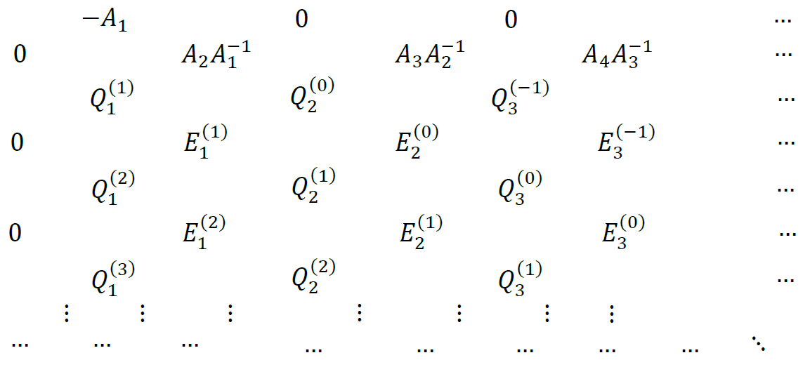
algorithm
where the are the spectral factors of . In addition, the algorithm gives all spectral factors simultaneously and in dominance order. We have chosen, in the above, the row generation algorithm because it is numerically stable see reference [[10]] for details.
Example 3.2.
Consider a matrix polynomial of order and degree with the following matrix coefficients.
| , |
| , |
We apply now the generalized row generation algorithm to find the complete set of spectral factors and then
we use the similarity transformations given by Shieh [[39]] to obtain the complete set of solvents both left and right equations(19)-(26).
Step 1: initialization of the program to start
Enter the degree and the order
Enter the number of iterations
Enter the matrix polynomial coefficients
Step 2: Construct and the first row of and first row of
Step 3: Building or generating the rest rows using the rhombus rules
Running the above steps (1) to (3) we obtain the following complete set of spectral factors :
Now, we should extract a complete set of right solvent from those block spectra using the algorithmic similarity
transformations in equations from (21) to (24).
Step 4: Reverse the orientation of spectral factors
Step 5:Evaluate the coefficients using the synthetic long division and then find the corresponding transformation matrix as in theorem 2.16.
You can verify the first solvent using:
rightzero1
Step 6: redo the same process for the next right solvents
For verification also you can use:
rightzero 2
Step 7:The last solvents are obtained directly from the most left spectral factor:
or by usinguse the transformation:
The final results are :
Finally, we can also obtain the corresponding complete set of left solvents using the algorithmic similarity
transformation described in equations from (10) to (12).
Step 8: coefficients determination using the synthetic long division
Step 9: find the corresponding similarity transformation matrix as in equations from equations (10) to (12).
The left solvents are now obtained:
3.2 Extended Horner algorithm
Horner’s method is a technique to evaluate polynomials quickly. It needs multiplications and additions and it is also a nested algorithmic programming that can decompose a polynomial into a multiplication of linear factors (Horner’s method) based on the Euclidian synthetic long division.
Similarly Horner’s method is a nesting technique requiring only multiplications and additions to evaluate an arbitrary -degree polynomial [[45]].
Theorem 3.3.
Let the function be the polynomial of degree defined on the real field where: are constant coefficients and is real variable.
| (40) |
If and
Then can be written as:
| (41) |
Where:
| (42) |
Proof.
The theorem can be proved using a direct calculation.
Identifying the coefficients of with different powers we get:
| where |
Now if is a root of the polynomial , then should be zero, and .
Hence, we may write
The algorithm of Horner method in its recursive formula is then:
∎
Now we generalize this nested algorithm to matrix polynomials, consider the monic -matrix
and according to theorem 2.8 the matrix can be factored as:
| (43) |
where
Using the algorithm of synthetic long division for matrices we obtain:
From the last two equations we can iterate the process to get recursive algorithm as follow:
Algorithm:
When you get the first spectral factor repeat the process until you get the complete set.
Example 3.4.
Consider a matrix polynomial of order and degree with the following matrix coefficients.
With
We apply now the extended Horner’s method via its algorithmic version to find the complete set of spectral factors and
then we use the similarity transformations given in [[23]] to obtain the complete set of left and right solvents
The Block Horner scheme is:
Running the above algorithm we obtain the next complete set of spectral factors:
Finally when we apply the similarity transformation algorithm as in equations from (21) to (24) to right (or left) solvent form we get:
3.2.1 Reformulation of the Block Horner method
An alternative form of the previous algorithm (under matrix and algebraic manipulations is:
Finally we obtain the following iterative formula:
| (44) |
Algorithm 3.5.
Enter the degree and the order
Enter the matrix polynomial coefficients
initial guess;
Give some small and (initial start)
While
Convergence condition: Using equations (44) we obtain the conditions for the the algorithm to converge to the solution.
1. Upper bound
Now if tends to constant matrix as and
with and then:
| (45) |
2. Lower bound
| (46) |
From eq. (45) and (46) we obtain:
| (47) |
Finally if the matrix tends to constant matrix and is nonsingular matrix then
is a solvent of the matrix polynomial .
Convergence Type: To get the convergence type we should evaluate a ratio relationship between any two successive differences.
| (48) |
We define then we have:
| (49) |
We know that:
| (50) |
from equations (49) and (50) we deduce that:
Finally:
| (51) |
Example 3.6.
consider the following matrix polynomial with repeated spectral factor:
With
Find such that
If we apply the Block Horner algorithm we find
Remark 3.7.
The Proposed Horner algorithm finds the whole set of spectral factors if it exists, even if there is no dominance factor among them.
3.2.2 Crossbred NewtonHorner method
In order to accelerate the Block Horner method we make a crossbred (Hybrid) Generalized Newton algorithm which is very fast due to its restricted local nature (i.e. Quadratic convergence).
Combine them we get:
| (52) |
where is the Frechet differential.
Definition 3.8.
Let and be Banach spaces and a nonlinear operator from to . If there exists a linear operator from to such that:
|
Then is called the Frechet derivative of at and sometimes is written . Also is read the Frechet derivative of at in the direction . And
Algorithm
Begin
3.2.3 Two stage Block Horner algorithm
To accelerate the block Horner algorithm we use now a two stage Newton like iteration. Now by using theorem 2.8 we obtain:
where and Now if is a solvent then If now assume that is a solvent to the matrix polynomial then and . Set also From the Horner scheme we can evaluate both and recursively:
| After iterating the last equation we get: | After iterating the last equation we get: |
Algorithm:
Remark 3.9.
this two stage algorithm gathers the two advantages of Horner sachem and Newton algorithm because it is nested programed nature, large sense independence on initial conditions and faster in execution due to the likeness or the conformity to Newton method.
Example 3.10.
Given the following matrix polynomial
Where:
We apply the two stage Horner algorithm and after 15 iterations we get:
With
3.2.4 Reformulation of the two stage Block Horner method
After back substitution of the nested programmed scheme and accumulation we obtain:
| and |
The two stage Block Horner Varian algorithm can be obtained when we use the compact forms of the matrices
and in term of lead us to Newton like iterated process.
Algorithm:
3.3 Comments
- •
A numerical method for solving a given problem is said to be local if it is based on local (simpler) model of the problem around the solution. From this definition, we can see that in order to use a local method, one has to provide an initial approximation of the solution. This initial approximation can be provided by a global method. As shown in Dahimene [[10]], local methods are fast converging while global ones are quite slow. This implies that a good strategy is to start solving the problem by using a global method and then refine the solution by a local method.
- •
The proposed hybrid or two stage Block-Horner’s algorithm converges rapidly as it performs a recursive iteration and is easily implemented in a digital computer. Horner’s algorithm could be used for evaluation of solvents of a matrix polynomial, but this method depends largely upon the initial guess even in some cases the initial value of is randomly chosen. Hence in sometimes it is very hard to find suitable solutions. Our algorithm is numerically more stable and its initial starting values are well defined and evaluated.
- •
The complete program starts with the algorithm. It is then followed by a refinement of the right factor by Horner’s algorithm. After deflation, Horner’s algorithm is again applied using the next output from the algorithm and the process is repeated until we find a linear term. The above process can be applied only to polynomial matrices that satisfy the conditions of theorem (i.e. complete right and left factorization and complete dominance relation between solvents).
- •
Many research works have been done on the spectral decomposition for matrix polynomials to achieve complete factorization and reconstruction of the block roots using algebraic and geometric numerical approaches, but (to our knowledge) nothing has been done for Block-Horner’s algorithm and/or Block- algorithm.
4 Application in control engineering
The system under examination is a power plant gas turbine (GE MS9001E) with single shaft, used as an electricity generator, installed in power station unit Sonelgaz at M’SILA, Algeria. The dynamic model of this gas turbine obtained via MIMO Recursive Least square estimator, using experimental inputs/outputs data acquired on-site and the obtained model is of order =6 with two inputs: (Output Pressure Compressor (OPC), and Output Temperature Compressor (OTC)), and two outputs: (Exhaust Temperature and Rotor Speed) [[46]]. In figure 2, the fundamental components of the system under study are given .
The dynamic model of this power plant gas turbine is a linear time invariant multi input multi output system,described by a set of high degree coupled vector differential equations with matrix constant coefficients(or a matrix transfer function). In our case the relationship between the input and output is a ratio of two matrix polynomials, expressed as a right (or left) matrix fraction description (RMFD or LMFD):
| (53) |
where: are matrix polynomials and stands for the operator. see [[4]],[[40]] and [[48]] and the reference therein . The obtained -matrix transfer function of the power plant gas turbine system is:
Where
We try to decouple the power plant gas turbine dynamic model. Let us first factorize (decompose) the numerator matrix polynomial into a complete set of spectral factors, then we use those block zeros into the denominator via state feedback. Hence the decoupling objectives are achieved.
Consider the square matrix transfer function:
with:
is an identity matrix and
,
Assume that can be factorized into Block zeros and can be factorized into Block roots (using one of the proposed algorithms):
| (54) |
| (55) |
The matrix transfer function can be written : . Also via the use of state feedback the control law becomes a state dependent and be rewritten as . Hence we obtain the following closed loop system:
where: and : are the desired spectral factors to be placed
Hence, the closed loop matrix transfer function is of the form:
| (56) |
In order to achieve perfect block decoupling we choose:
Now by assigning those block roots the system is decoupled and the closed loop matrix transfer function is:
| (57) |
Now we should construct the numerator and denominator matrix polynomials of the gas turbine system from the matrix transfer function (see [[13],[14] and [17]]):
where:
Let we decompose the numerator and denominator matrix polynomials and reconstruct their block roots:
and
The Block spectral factors are approximately computerized with a residual normed tolerance error given by:
and
Remark 4.1.
The last Block pole can be constructed using the synthetic long division.
Figure (3) illustrates a comparison between the proposed algorithms in term of the convergence speed and residual normed tolrance error.
The numerator block zeros are computed using the proposed algorithms compared to recent developed method called the generalized secant method [[49]] which can factorize matrix polynomial into a complete set of block roots. Numerical results of the developed procedures as illustrated in [[49]] give:
Although the Block Newton method aims to improve the convergence speed over the Block Horner method, it cannot always achieve this goal. The Newton-Horner’s method converges quadratically due to its conformity to Newton method. As a consequence, the number of significant values is roughly doubled every iteration, provided that is close to the root . The two stage algorithm is the best method of finding roots, it is simple and fast (at first seven iterations the average error becomes and ). The only drawback of the two stage method is that it uses the matrix inversion, and partially is dependent on the initial guess. Our refinement algorithm avoided this obstacle. As indicated in figure (2) the Q-D algorithm converges, but it is of global nature with no initial independence. The global convergence characteristics of the secant method are poor, as indicated in this figure.
The desired denominator is of third order written in the form:
Using the prescribed decoupling algorithm we obtain:
Where:
The state feedback gain matrix of the Block controller form is obtained by see [[47]],[[48]]:
Now let we go back to original base by similarity transformation as found in [[4]],[[40]] and [[48]]:
The new model of the decoupled system after state feedback is:
Based on the results we deduce that the Block roots are well computed, both numerator and denominator matrix polynomials ( and ) are perfectly decomposed using the proposed procedure.
4.1 Suggestions for further research
The results obtained during this research work arose many questions and problems which are subject for future research
- •
Finding other globalization techniques for the Block-Horner’s algorithm to avoid the local restriction and the problem of initial guess, so to arrive at very fast global nested program. Also exploring and extending other scalar numerical methods to factorize matrix polynomials.
- •
Both of The Block-Horner’s algorithm and the Block- algorithm as used in our work converges to factors of a matrix polynomial. By using the defined similarity transformations, we can derive the solvents. However, it would be convenient to have a global algorithm that converges rapidly and directly to all solvents.
- •
If a column in the tableau converges, it implies that there exists a factorization of the matrix polynomial that splits the spectrum into a dominant set and a dominated one. If the system under consideration is a digital system, we know that the largest modulus latent roots affect the dynamic properties of the system. In such case, the algorithm can become a tool for system reduction (using the dominant mode concept).
- •
The computational procedure for finding the solvents of a matrix polynomial with repeated block roots (solvents) and/or spectral factors need to be investigated further.
5 Conclusion
In this paper we have introduced new numerical approaches for determining the complete sets of spectral factors and
solvents of a monic matrix polynomial. For avoiding the initial guess we have proposed a systematic method for
the Block-Horner’s algorithm via a refinement of the Block- algorithm. At least three advantages are offeedr by
the proposed technique: (i) an algorithm with global nature is obtained; hence there is no initial-guess problem
during the whole procedure, (ii) high speed convergence to each solution and only a few iterations are required
(iii) via the help of refinement and direct cascading, the algorithms are easily coupled together and the whole
scheme is suitable for programming in a digital computer digital. The obtained solvents can be
considered as a useful tool for carrying out the block partial fraction expansion for the inverse of a matrix
polynomial. Those partial fractions are matrix transfer functions of reduced order linear systems such
that the realization of them leads to block diagonal (block-decoupling) or parallel decomposed multivariable linear
time invariant system. The dynamic properties of MIMO systems depend on block pole of its characteristic matrix polynomial. Therefore they can be used as tools for block-pole placement, block-system identification and block-model order reduction. In addition, the proposed
method can be employed to carry out the block spectral factorization of a matrix polynomial for problems in optimal
control, filtering and estimation.
Acknowledgement
Dr. George F. Fragulis work is supported by the program Rescom 80159 of the Univ. of Applied Science of Western Macedonia, Hellas.
References
- [1] J. J. DiStefano, A. R. Stubberud, I. J. Williams,Theory and Problems of Feedback and Control Systems, Mc. Graw Hill, 1967.
- [2] B. N. Parlett, The LU and QR Algorithms, in Ralston and Wilf, Mathematical Methods for Digital Computers, Vol. 2, John Wiley, 1967.
- [3] Bachir Nail, Abdellah Kouzou,Ahmed Hafaifa, Parametric Identification of Multivariable Industrial System Using Left Matrix Fraction Description, J. Automation and Systems Engineering 10-4 (2016): 221-230
- [4] Malika Yaici, Kamel Hariche, On eigenstructure assignment using block poles placement, European Journal of Control, May 2014.
- [5] Malika Yaici, Kamel Hariche,Clark Tim, A Contribution to the Polynomial Eigen Problem, International Journal of Mathematics, Computational, Natural and Physical Engineering, Vol:8 No 10, 2014.
- [6] Nicholas J. Higham,Function of Matrices: theory and computation,SIAM 2008.
- [7] George F. Fragulis Transformation of a PMD into an implicit system using minimal realizations of its transfer function matrix in terms of finite and infinite spectral data, Journal of the Franklin Institute, vol.333, pages 41-56, 1996.
- [8] George F. Fragulis Generalized Cayley-Hamilton theorem for polynomial matrices with arbitrary degree, International Journal of Control, vol.62, pages 1341-1349, 1995.
- [9] B.G. Mertzios and George F. Fragulis The fundamental matrix in ARMA systems, IEEE International Conference on Industrial Technology, pages 1541-1542, 2004.
- [10] A.Dahimene,Algorithms for the factorization of matrix polynomials, Master Thesis INELEC , 1992.
- [11] A.Dahimene, Incomplete matrix partial fraction expansion, Control and Cybernetics vol. 38 (2009) No.3
- [12] S. M. Ahn, Stability of a Matrix Polynomial in Discrete Systems, IEEE trans. on Auto. Contr., Vol. AC-27, pp. 1122-1124, Oct. 1982.
- [13] C. T. Chen, Linear System Theory and Design, Holt, Reinhart and Winston, 1984.
- [14] T. Kailath, W. Li, Linear Systems,Prentice Hall, 1980.
- [15] V. Kucera, Discrete Linear Control: The Polynomial Equation Approach,John Wiley, 1979.
- [16] P. Resende, E. Kaskurewicz, A Sufficient Condition for the Stability of Matrix Polynomials,IEEE trans, on. Auto. Contr., Vol. AC-34, pp. 539-541, May 1989.
- [17] Leang S. Shieh, F. R Chang, B. C. Mcinnis, The Block partial fraction expansion of a matrix fraction description with repeated blocl poles, IEEE Trans. Auto. Cont. AC-31, pp. 236-239, 1986.
- [18] E. D. Denman and A. N. Beavers, The matrix sign function and computations in systems,Appl. Math. Comput. 2:63-94 (1976).
- [19] M. K. Solak, Divisors of Polynomial Matrices: Theory and Applications,IEEE trans. on Auto. Contr., Vol. AC-32, pp. 916-919, Oct. 1987.
- [20] J. E. Dennis, J. F. Traub, and R. P. Weber, Algorithms for solvents of matrix polynomials,SZAhlJ. Numer. Anal. 15:523-533 (1978).
- [21] E. D. Denman, Matrix polynomials, roots, and spectral factors, A . Math. Comput. 3:359-368, (1977).
- [22] L. S. Shieh, S. Sacheti, A Matrix in the Block Schwarz Form and the Stability of Matrix Polynomials,Int. J. Control, Vol. 27, pp. 245-259, 1978.
- [23] L. S. Shieh, Y. T. Tsay, and N. I’. Coleman, Algorithms for solvents and spectral factors of matrix polynomials,Internat. 1. Control 12:1303-1316 (1981).
- [24] L. S. Shieh and Y. T. Tsay, Transformation of solvent and spectral factors of matrix polynomial, and their applications,Internat. J. Control 34:813-823 (1981).
- [25] J. S. H. Tsai, I,. S. Shieh, and T. T. C. Shen, Block power method for computing solvents and spectral factors of matrix polynomials,Internut. Computers and Math. Appl. 16:683-699 (1988).
- [26] P. Henrici,The Quotient-Difference Algorithm,Nat. Bur. Standards Appl. Math. Series, Vol. 49, pp. 23-46, 1958.
- [27] L. S. Shieh, F. R. Chang, and B. C. Mcinnis, The block partial fraction expansion of a matrix fraction description with repeated block poles,IEEE Trans. Automut. Control. 31:23-36 (1986).
- [28] J. E. Dennis, J. F. Traub, and R. P. Weber, The algebraic theory of matrix polynomials,SZAlZl J. Numer. Anal. 13:831-845 (1976).
- [29] L. S. Shieh and Y. T. Tsay, Block modal matrices and their applications to multivariable control systems,IEE Proc. D, Control Theory Appl. 2:41-48(1982).
- [30] L. S. Shieh and N. Chahin, A computer-aided method for the factorization of matrix polynomials,Internat. Systems Sci. 12:1303-1316 (1981).
- [31] J. S. H. Tsai and C. M. Chen and L. S. Shieh, A Computer-Aided Method for Solvents and Spectral Factors of Matrix Polynomials,Applied mathematics and computation 47:211-235 (1992).
- [32] K. Hariche, Interpolation Theory in the Structural Analysis of -matrices: Chapter3, Ph. D. Dissertation, University of Houston, 1987.
- [33] R. L. Burden and J. D. Faires,Numerical Analysis , 8th Edition, Thomson Brooks/Cole, Belmont, CA, USA, 2005.
- [34] L. S. Shieh and Y. T. Tsay, Transformation of a class of multivariable control systems to block companion forms,IEEE Truns. Autonwt. Control 27: 199-203 (1982).
- [35] K. Hariche, E. D. Denman, interpolation Theory and -Matrices, journal of mathematical analysis and applications 143, 53 and 547 (1989).
- [36] K. Hariche and E. D. Denman, On Solvents and Lagrange Interpolating -Matrices, applied mathematics and computation 25321-332 (1988).
- [37] E. Periera, On solvents of matrix polynomials, Appl. Numer. Math., vol. 47, pp. 197-208, 2003.
- [38] E. Periera,Block eigenvalues and solution of differential matrix equation, mathematical notes, Miskolc, Vol. 4, No.1 (2003), pp. 45-51.
- [39] L. S. Shieh and Y. T. Tsay, Algebraic-geometric approach for the modal reduction of large-scale multivariable systems,IEE Proc. D Control Theory Appl. 131(1):23-26 (1984).
- [40] Malika Yaici, Kamel Hariche,On Solvents of Matrix Polynomials, International Journal of Modeling and Optimization, Vol. 4, No. 4, August 2014.
- [41] I. Gohberg, P. Lancaster, L. Rodman, Matrix Polynomials,Academic Press, 1982.
- [42] A. Pathan and T. Collyer, The wonder of Horner’s method,Mathematical Gazette, 87 (2003), No. 509, 230-242.
- [43] H. Zabot, K. Hariche, On solvents-based model reduction of MIMO systems, International Journal of Systems Science, 1997, volume 28, number 5, pages 499-505.
- [44] S. Barnett,Matrices in Control Theory,Van Nostrand Reinhold, New York, 1971.
- [45] I. Gohberg, M. A. Kaashoek, and L. Rodman, Spectral analysis of operator polynomial and a generalized Vandermonde matrix,1. the finite-dimensional case, in Topics in Functional Analysis, Academic, 1978, pp. 91-128.
- [46] B. Bekhiti, A. Dahimene, B. Nail, K. Hariche, and A. Hamadouche, On Block Roots of Matrix Polynomials Based MIMO Control System Design, International Conference on Electrical Engineering ICEE Boumerdes , 2015.
- [47] Carl D. Meyer,Matrix Analysis and Applied Linear Algebra,SIAM 2000.
- [48] Yih T. Tsay and Leang S. Shieh Block decompositions and block modal controls of multivariable control systems, Autoraatica, Vol. 19, No.1, pp. 29-40, 1983.
- [49] Marlliny Monsalve and Marcos Raydan, Newton’s method and secant methods: A longstanding relationship from vectors to matrices Portugaliae Mathematica European Mathematical Society, Vol. 68, Fasc. 4, 2011, 431–475 6 DOI 10.4171/PM/1901