Relativistic stars in degenerate higher-order scalar-tensor theories after GW170817

The nearly simultaneous detection of gravitational waves GW170817 and the $\gamma$-ray burst GRB 170817A [1, 2, 3] places a very tight constraint on the speed of gravitational waves, $c_{\rm GW}$. The deviation of $c_{\rm GW}$ from the speed of light is less than 1 part in $10^{15}$. This can be translated to constraints on modified gravity such as scalar-tensor theories, vector-tensor theories, massive gravity, and Hořava gravity [4, 5, 6, 7, 8, 9]. In particular, in the context of the Horndeski theory (the most general scalar-tensor theory having second-order equations of motion¹¹ 1 The original form of the Horndeski action is different from its modern expression obtained by extending the Galileon theory [10]. The equivalence of the two apparently different theories was shown in [11].) [12], two of the four free functions in the action are strongly constrained, leaving only the simple, traditional form of nonminimal coupling of the scalar degree of freedom to the Ricci scalar, i.e., the “$f(\phi){\cal R}$”-type coupling.

However, it has been pointed out that there still remains an interesting, nontrivial class of scalar-tensor theories beyond Horndeski that can evade the gravitational wave constraint as well as solar-system tests [4, 6, 5, 13, 14, 15, 16, 17, 18]. Such theories have higher-order equations of motion as they are more general than the Horndeski theory, but the system is degenerate and hence is free from the dangerous extra degree of freedom that causes Ostrogradski instability. Earlier examples of degenerate higher-order scalar-tensor (DHOST) theory are found in [19, 20], and the degeneracy conditions are systematically studied and classified at quadratic order in second derivatives of the scalar field in [21, 22] and at cubic order in [23]. Degenerate theories can also be generated from nondegenerate ones via noninvertible disformal transformation [24, 25].

One of the most interesting phenomenologies of DHOST theories is efficient Vainshtein screening outside matter sources and its partial breaking in the inside [26]. The partial breaking of screening modifies, for instance, stellar structure [27, 28]. This fact was used to test DHOST theories, or, more specifically, the Gleyzes-Langlois-Piazza-Vernizzi (GLPV) subclass [20], against astrophysical observations [29, 30, 31, 32, 33, 34]. Going beyond the weak-field approximation, relativistic stars in the GLPV theory have been studied in [35, 36].

In this paper, we consider relativistic stars in DHOST theories that are more general than the GLPV theory but evade the constraint on the speed of gravitational waves [4, 5, 6]. So far, this class of theories have been investigated by employing the weak-field approximation [13, 14, 16] and in a cosmological context [17]. Very recently, compact objects including relativistic stars in the GLPV theory with $c_{\rm GW}=1$ have been explored in Ref. [37].

This paper is organized as follows. In the next section, we introduce the DHOST theories with $c_{\rm GW}=1$ and derive the basic equations describing a spherically symmetric relativistic star. To check the consistency with the previous results, we linearize the equations and see the gravitational potential in the weak-field approximation in Sec. III. Then, in Sec. IV, we give boundary conditions imposed at the stellar center and in the exterior region. Our numerical results are presented in Sec. V. We draw our conclusions in Sec. VI. Since some of the equations are quite messy, their explicit expression is shown in Appendix A.

The action of the quadratic DHOST theory we study is given by

where ${\cal R}$ is the Ricci scalar, $X:=\phi_{\mu}\phi^{\mu}$, and

with $\phi_{\mu}=\nabla_{\mu}\phi$ and $\phi_{\mu\nu}=\nabla_{\mu}\nabla_{\nu}\phi$. The functions $A_{I}(X)$ must be subject to certain conditions in order for the theory to be degenerate and satisfy $c_{\rm GW}=1$, as explained shortly. Here, shift symmetry is assumed and the other possible terms of the form $G_{2}(X)$ and $G_{3}(X)\Box\phi$ are omitted. In particular, we do not include the usual kinetic term $-X/2$ in this paper.²² 2 The inclusion of the usual kinetic term $-X/2$ gives rise to an interesting branch of asymptotically locally flat solutions with a deficit angle, as has been recently explored in Ref. [37]. We leave this possibility for future research. The appearance of a deficit angle in the GLPV theory was pointed out earlier in Refs. [38, 39]. As we will see, our ansatz for the scalar field is different from that assumed in Refs. [38, 39] (see Eq. (13) below). Probably this is the reason why we can obtain spherically symmetric solutions that are regular at the center. These assumptions are nothing to do with the degeneracy conditions and the $c_{\rm GW}=1$ constraint to be imposed below. However, with this simplification one can concentrate on the effect of Vainshtein breaking.

Note in passing that the DHOST theories are equivalent to the Horndeski theory with disformally coupled matter. Therefore, the setup we are considering is in some sense similar to that explored in Ref. [40]. However, the crucial difference is that, in contrast to Ref. [40], our theory corresponds to the case where the conformal and disformal coupling functions depend on the first derivative of the scalar field.

We require that the speed of gravitational waves, $c_{\rm GW}$, is equal to the speed of light [2]. In our theory $c_{\rm GW}$ is given by $c_{\rm GW}^{2}=f/(f-XA_{1})$ [41], so that

The degeneracy conditions read

We thus have two free functions, $A_{3}$ and $f$, in the quadratic DHOST sector with $c_{\rm GW}=1$. This theory has been explored recently in Refs. [4, 5, 6, 7, 13, 14, 16, 17]. (See Ref. [18] for a different subclass with $f=\;$const and $A_{2}=-A_{1}\neq 0$.) Following Ref. [17], we introduce

and use this instead of $A_{3}$. In the special case with $B_{1}=0=A_{5}$, the action reduces to that of the GLPV theory.

We consider a static and spherically symmetric metric,

The scalar field is taken to be

where $v\,(\neq 0)$ is a constant. Even though $\phi$ is linearly dependent on the time coordinate, it is consistent with the static spacetime because the action (1) possess a shift symmetry, $\phi\to\phi+c$, and $\phi$ without derivatives does not appear in the field equations. This ansatz was also used to obtain black hole solutions in the Galileon and Horndeski theories in Refs. [42, 43, 44, 45, 46].

The field equations are given by

where ${\cal E}_{\mu\nu}$ is obtained by varying the action with respect to the metric and $J^{\mu}$ is the shift current defined by $\sqrt{-g}J^{\mu}=\delta S/\delta\phi_{\mu}$. The energy-momentum tensor is of the form

The radial component of the conservation equations, $\nabla_{\mu}T^{\mu}_{\nu}=0$, reads

where ${}^{\prime}:={\rm d}/{\rm d}r$.

With direct calculation we find that

Therefore, the gravitational field equation ${\cal E}_{tr}=0$ requires that $J^{r}$ vanishes. Then, the field equation for the scalar field (15) is automatically satisfied.

To write Eq. (14) and $J^{r}=0$ explicitly, it is more convenient to use $X=-e^{-\nu}v^{2}+e^{-\lambda}\psi^{\prime 2}$ instead of $\psi$. In terms of $X$, we have

where

but the explicit expression of $\widetilde{{\cal E}}_{t}$, $\widetilde{{\cal E}}_{r}$, and $\widetilde{{\cal E}}_{J}$ are messy.

We see that ${\cal E}_{r}^{r}$ and $\psi^{\prime}J^{r}$ have the same coefficients $c_{1}$ and $c_{2}$. Moreover, we find by an explicit computation that ${\cal E}_{r}^{r}$ and $\psi^{\prime}J^{r}$ are linearly dependent on $\lambda^{\prime}$ and their coefficients are also the same. Therefore, by taking the combination ${\cal E}_{r}^{r}-\psi^{\prime}J^{r}$ one can remove $\nu^{\prime\prime}$, $X^{\prime\prime}$, and $\lambda^{\prime}$. Then, the field equation ${\cal E}_{r}^{r}-\psi^{\prime}J^{r}=P$ can be solved for $\lambda$ to give

where

Using Eq. (26), we can eliminate $\lambda$ and $\lambda^{\prime}$ from Eqs. (19) and (21). In doing so we replace $P^{\prime}$ with $\nu^{\prime}$, $\rho$, and $P$ by using Eq. (17). We then obtain

where $k_{1,2}=k_{1,2}(\nu,\nu^{\prime},X,X^{\prime},P)$. The field equation ${\cal E}_{t}^{t}+\rho=0$ can also be written in the form

Note that we have the same coefficients $k_{1}$ and $k_{2}$. This is due to the degeneracy conditions. We thus arrive at a first-order equation, ${\cal J}_{1}={\cal J}_{2}$, which can be solved for $X^{\prime}$ as

where ${\cal F}_{1}$ and ${\cal F}_{2}$ are complicated. Their explicit form is presented in Appendix A. Finally, we use Eq. (30) to eliminate $X^{\prime}$ and $X^{\prime\prime}$ from Eq. (28). This manipulation also removes $\nu^{\prime\prime}$, as it should be because the theory is degenerate. We thus arrive at

where the explicit expression of ${\cal F}_{3}$ is extremely long and is presented in Appendix A.

We have thus obtained our basic equations describing the Tolman-Oppenheimer-Volkoff system in DHOST theories. Given the equation of state relating $\rho$ and $P$, one can integrate Eqs. (17), (30), and (31) to determine $P=P(r)$, $\nu=\nu(r)$, and $X=X(r)$. Equation (26) can then be used to obtain $\lambda=\lambda(r)$.

Since our procedure to obtain spherically symmetric solutions is different from that of previous works [13, 14, 16, 17], it is a good exercise to check here that one can reproduce the previous result in a nonrelativistic, weak-field limit.

We write

and derive linearized equations for a nonrelativistic source with $P=0$. It is straightfoward to derive

where we introduced

and

We will see below that $G_{N}$ can indeed be regarded as the Newton constant. We then solve the following set of equations:

Combining Eqs. (40) and (41), the following second-order equation for $\delta\nu$ can be derived,

where $M(r)$ is the enclosed mass defined as

Equation (42) can be integrated to give

where $C_{0}$ is an integration constant. Combining Eqs. (40) and (41) again, we obtain

Finally, we use Eq. (39) to get

where

Imposing regularity at the center, we take $C_{0}=0$.

We may set $M^{\prime}=0$ and $M^{\prime\prime}=0$ outside the source, and then we have $\delta\nu=-\delta\lambda=-2G_{N}M/r$, which coincides with the solution in general relativity if $G_{N}$ is identified as the Newton constant. Gravity is modified only inside the matter source, and we have seen that there are three parameters, $\Upsilon_{1,2,3}$, that characterize the deviation from the standard result. They are subject to

so that actually only two of them are independent. Note that in the case of the GLPV theory, one has $B_{1}=0$, and hence $\Upsilon_{2}=2\Upsilon_{1}/5$ and $\Upsilon_{3}=0$.

To see that the previous result is correctly reproduced, we perform a small coordinate transformation

The metric then takes the form

where

Thus, we can confirm that Eq. (52) reproduces the previous result found in the literature [13, 14, 16, 17].

Constraints on the $\Upsilon$ parameters have been obtained from astrophysical observations in the case of $\Upsilon_{3}=0$ [27, 29, 30, 31, 32, 33, 34, 35, 36]. For example, the mass-radius relation of white dwarfs yields the constraint $-0.18<\Upsilon_{1}<0.27$ [31]. This is valid even in the case of $\Upsilon_{3}\neq 0$, because the constraint comes only from $\Phi$ in such nonrelativistic systems. To probe $\Psi$, one needs nonrelativistic systems and/or observations based on propagation of light rays such as gravitational lensing, and a tighter constraint has been imposed on $\Upsilon_{1}$ combining the information on $\Psi$ [32]. However, this relies on the assumption that $\Upsilon_{3}=0$. For this reason, it is important to study relativistic stars in theories with $\Upsilon_{3}\neq 0$.

Another constraint can be obtained from the Hulse-Taylor pulsar, which limits the difference between $G_{N}$ and the effective gravitational coupling for gravitational waves, $G_{\rm GW}=1/16\pi f(-v^{2})$ [47]. The constraint reads [16]

Note, however, that this constraint is based on the assumption that the scalar radiation does not contribute to the energy loss, whose validity must be ascertained in the Vainshtein-breaking theories.

As a specific example, we study the model of Ref. [17]:

where $\alpha$ and $\beta$ are constants. Note that we are using the notation such that $8\pi G_{N}\neq M_{\rm Pl}^{-2}$. We have

and hence the model with $\beta\neq 0$ is more general than the GLPV theory. For this choice of the functions the degeneracy conditions (9) and (10) leads to

This model, with the addition of the lower order Horndeski terms, admits viable self-accelerating cosmological solutions [17], and therefore is interesting.

Hereafter we will use the dimensionless parameters defined as

The parameters that characterize Vainshtein breaking in the Newtonian regime, $\Upsilon_{i}$, can then be estimated as

From Eq. (53) we also estimate

Therefore, by taking sufficiently small $\overline{\alpha}$ and $\overline{\beta}$ (say, ${\cal O}(10^{-3})$), current constraints can be evaded. In the following numerical calculations, we will employ such small values of the parameters.

The equation of state we use is given by

with $K=7.73\times 10^{-3}\,(8\pi G_{N})^{3}M_{\odot}^{2}$ ($K=123\,M_{\odot}^{2}$ in the units where $G_{N}=1$), which has been used frequently in the modifed gravity literature [48, 49, 50, 51, 35]. With this simple equation of state we focus on the qualitative nature of the solutions.

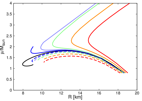
We start with the theories with $\overline{\beta}=0$ and focus on the effect of $\overline{\alpha}$. Figures 1 and 2 show the mass ($\mu$) versus central density relation and the mass versus radius relation, respectively. In all cases $\overline{\alpha}$ is taken to be very small so that the Vainshtein-breaking effect is not significant in the Newtonian regime. It can be seen that for fixed $\rho_{c}$ or $R$ the mass is larger (smaller) for $\overline{\alpha}>0$ ($\overline{\alpha}<0$) than in the case of general relativity (GR). Interestingly, there is a maximum central density, $\rho_{c,{\rm max}}$, above which no solution can be found. This property is similar to what was found in Ref. [48], where the subclass of the Horndeski theory having derivative coupling to the Einstein tensor was studied. For $\overline{\alpha}\lesssim 2\times 10^{-4}$, we see that $\mu<\infty$ as $\rho_{c}\to\rho_{c,{\rm max}}$, but for $\overline{\alpha}\gtrsim 2\times 10^{-4}$ we find that $\mu\to\infty$ and $R\to\infty$ as $\rho_{c}\to\rho_{c,{\rm max}}$. Therefore, in the latter case there are solutions at high densities that are very different from relativistic stars in GR. Note that this occurs even for a tiny value of $\overline{\alpha}$.

Next, we fix $\overline{\alpha}=0$ and draw the same diagrams for different (small) values of $\overline{\beta}$. The results are presented in Figs. 3 and 4, which are seen to be qualitatively similar to Figs. 1 and 2, respectively. Therefore, although $\overline{\beta}$ is supposed to signal the “beyond GLPV” effects, they are not manifest and the roles of the two parameters $\overline{\alpha}$ and $\overline{\beta}$ in relativistic stars are qualitatively similar. We have performed numerical calculations for more general cases with $\overline{\alpha}\neq 0$ and $\overline{\beta}\neq 0$, and confirmed that they also lead to qualitatively similar results.

Just for reference some examples of radial profiles of the metric and $X$ in the stellar interior are presented in Figs. 5 and 6 for $(\overline{\alpha},\overline{\beta})=(\pm 2\times 10^{-3},0)$ and in Figs. 7 and 8 for $(\overline{\alpha},\overline{\beta})=(0,\pm 2\times 10^{-3})$. As mentioned in Sec. IV.3, one can find that $X^{\prime}$ is nonvanishing at the surface, leading to the discontinuity of $X^{\prime}$, and that $e^{-\lambda}$ does not agree with $e^{\nu}$ there in Fig. 7, indicating the discontinuity of $e^{-\lambda}$ since $e^{\nu}$ must be continuous.

In this paper, we have studied the Tolman-Oppenheimer-Volkoff system in degenerate higher-order scalar-tensor (DHOST) theory that is consistent with the GW170817 constraint on the speed of gravitational waves. Although the field equations are apparently of higher order, we have reduced them to a first-order system by combining the different components. This is possible because the theory we are considering is degenerate.

In DHOST theories that are more general than Horndeski, breaking of the Vainshtein screening mechanism occurs inside matter [26, 13, 14, 16], which would modify the interior structure of stars. Assuming a simple concrete model of DHOST theory with two parameters and the equation of state, we have solved numerically the field equations. The parameters were chosen so that the Vainshtein-breaking effect in the Newtonian regime is suppressed by the factor $\Upsilon_{i}\lesssim 10^{-3}$. Nevertheless, we have found a possible large modification in the mass-radius relation. This is significant in particular at densities as high as the maximum above which no solutions can be obtained.

In this paper, we have focused on the rather qualitative nature of relativistic stars in the DHOST theory, but it would be important to employ more realistic equations of state for testing the theory against astrophysical observations. This is left for further study. It would be also interesting to explore to what extent the modification to the stellar structure depends on the concrete form of the DHOST Lagrangian. We hope to come back to this question in a future study.

References

- [1] B. P. Abbott et al. [LIGO Scientific and Virgo Collaborations], “GW170817: Observation of Gravitational Waves from a Binary Neutron Star Inspiral,” Phys. Rev. Lett. 119, no. 16, 161101 (2017) [arXiv:1710.05832 [gr-qc]].
- [2] B. P. Abbott et al. [LIGO Scientific and Virgo and Fermi-GBM and INTEGRAL Collaborations], “Gravitational Waves and Gamma-rays from a Binary Neutron Star Merger: GW170817 and GRB 170817A,” Astrophys. J. 848, no. 2, L13 (2017) [arXiv:1710.05834 [astro-ph.HE]].
- [3] B. P. Abbott et al. “Multi-messenger Observations of a Binary Neutron Star Merger,” Astrophys. J. 848, no. 2, L12 (2017) [arXiv:1710.05833 [astro-ph.HE]].
- [4] P. Creminelli and F. Vernizzi, “Dark Energy after GW170817 and GRB170817A,” Phys. Rev. Lett. 119, no. 25, 251302 (2017) [arXiv:1710.05877 [astro-ph.CO]].
- [5] J. Sakstein and B. Jain, “Implications of the Neutron Star Merger GW170817 for Cosmological Scalar-Tensor Theories,” Phys. Rev. Lett. 119, no. 25, 251303 (2017) [arXiv:1710.05893 [astro-ph.CO]].
- [6] J. M. Ezquiaga and M. Zumalacárregui, “Dark Energy After GW170817: Dead Ends and the Road Ahead,” Phys. Rev. Lett. 119, no. 25, 251304 (2017) [arXiv:1710.05901 [astro-ph.CO]].
- [7] T. Baker, E. Bellini, P. G. Ferreira, M. Lagos, J. Noller and I. Sawicki, “Strong constraints on cosmological gravity from GW170817 and GRB 170817A,” Phys. Rev. Lett. 119, no. 25, 251301 (2017) [arXiv:1710.06394 [astro-ph.CO]].
- [8] A. Emir Gümrükçüoğlu, M. Saravani and T. P. Sotiriou, “Hořava gravity after GW170817,” Phys. Rev. D 97, no. 2, 024032 (2018) doi:10.1103/PhysRevD.97.024032 [arXiv:1711.08845 [gr-qc]].
- [9] J. Oost, S. Mukohyama and A. Wang, “Constraints on Einstein-aether theory after GW170817,” arXiv:1802.04303 [gr-qc].
- [10] C. Deffayet, X. Gao, D. A. Steer and G. Zahariade, “From k-essence to generalised Galileons,” Phys. Rev. D 84, 064039 (2011) [arXiv:1103.3260 [hep-th]].
- [11] T. Kobayashi, M. Yamaguchi and J. Yokoyama, “Generalized G-inflation: Inflation with the most general second-order field equations,” Prog. Theor. Phys. 126, 511 (2011) [arXiv:1105.5723 [hep-th]].
- [12] G. W. Horndeski, “Second-order scalar-tensor field equations in a four-dimensional space,” Int. J. Theor. Phys. 10, 363 (1974).
- [13] M. Crisostomi and K. Koyama, “Vainshtein mechanism after GW170817,” Phys. Rev. D 97, no. 2, 021301 (2018) [arXiv:1711.06661 [astro-ph.CO]].
- [14] D. Langlois, R. Saito, D. Yamauchi and K. Noui, “Scalar-tensor theories and modified gravity in the wake of GW170817,” arXiv:1711.07403 [gr-qc].
- [15] E. Babichev, C. Charmousis, G. Esposito-Farèse and A. Lehébel, “Stability of a black hole and the speed of gravity waves within self-tuning cosmological models,” arXiv:1712.04398 [gr-qc].
- [16] A. Dima and F. Vernizzi, “Vainshtein Screening in Scalar-Tensor Theories before and after GW170817: Constraints on Theories beyond Horndeski,” arXiv:1712.04731 [gr-qc].
- [17] M. Crisostomi and K. Koyama, “Self-accelerating universe in scalar-tensor theories after GW170817,” arXiv:1712.06556 [astro-ph.CO].
- [18] N. Bartolo, P. Karmakar, S. Matarrese and M. Scomparin, “Cosmic structures and gravitational waves in ghost-free scalar-tensor theories of gravity,” arXiv:1712.04002 [gr-qc].
- [19] M. Zumalacárregui and J. García-Bellido, “Transforming gravity: from derivative couplings to matter to second-order scalar-tensor theories beyond the Horndeski Lagrangian,” Phys. Rev. D 89, 064046 (2014) [arXiv:1308.4685 [gr-qc]].
- [20] J. Gleyzes, D. Langlois, F. Piazza and F. Vernizzi, “Healthy theories beyond Horndeski,” Phys. Rev. Lett. 114, no. 21, 211101 (2015) [arXiv:1404.6495 [hep-th]].
- [21] D. Langlois and K. Noui, “Degenerate higher derivative theories beyond Horndeski: evading the Ostrogradski instability,” JCAP 1602, no. 02, 034 (2016) [arXiv:1510.06930 [gr-qc]].
- [22] M. Crisostomi, K. Koyama and G. Tasinato, “Extended Scalar-Tensor Theories of Gravity,” JCAP 1604, no. 04, 044 (2016) [arXiv:1602.03119 [hep-th]].
- [23] J. Ben Achour, M. Crisostomi, K. Koyama, D. Langlois, K. Noui and G. Tasinato, “Degenerate higher order scalar-tensor theories beyond Horndeski up to cubic order,” JHEP 1612, 100 (2016) [arXiv:1608.08135 [hep-th]].
- [24] K. Takahashi and T. Kobayashi, “Extended mimetic gravity: Hamiltonian analysis and gradient instabilities,” JCAP 1711, no. 11, 038 (2017) [arXiv:1708.02951 [gr-qc]].
- [25] D. Langlois, M. Mancarella, K. Noui and F. Vernizzi, “Mimetic gravity as DHOST theories,” arXiv:1802.03394 [gr-qc].
- [26] T. Kobayashi, Y. Watanabe and D. Yamauchi, “Breaking of Vainshtein screening in scalar-tensor theories beyond Horndeski,” Phys. Rev. D 91, no. 6, 064013 (2015) [arXiv:1411.4130 [gr-qc]].
- [27] K. Koyama and J. Sakstein, “Astrophysical Probes of the Vainshtein Mechanism: Stars and Galaxies,” Phys. Rev. D 91, 124066 (2015) [arXiv:1502.06872 [astro-ph.CO]].
- [28] R. Saito, D. Yamauchi, S. Mizuno, J. Gleyzes and D. Langlois, “Modified gravity inside astrophysical bodies,” JCAP 1506, 008 (2015) [arXiv:1503.01448 [gr-qc]].
- [29] J. Sakstein, “Hydrogen Burning in Low Mass Stars Constrains Scalar-Tensor Theories of Gravity,” Phys. Rev. Lett. 115, 201101 (2015) [arXiv:1510.05964 [astro-ph.CO]].
- [30] J. Sakstein, “Testing Gravity Using Dwarf Stars,” Phys. Rev. D 92, 124045 (2015) [arXiv:1511.01685 [astro-ph.CO]].
- [31] R. K. Jain, C. Kouvaris and N. G. Nielsen, “White Dwarf Critical Tests for Modified Gravity,” Phys. Rev. Lett. 116, no. 15, 151103 (2016) [arXiv:1512.05946 [astro-ph.CO]].
- [32] J. Sakstein, H. Wilcox, D. Bacon, K. Koyama and R. C. Nichol, “Testing Gravity Using Galaxy Clusters: New Constraints on Beyond Horndeski Theories,” JCAP 1607, no. 07, 019 (2016) [arXiv:1603.06368 [astro-ph.CO]].
- [33] J. Sakstein, M. Kenna-Allison and K. Koyama, “Stellar Pulsations in Beyond Horndeski Gravity Theories,” JCAP 1703, no. 03, 007 (2017) [arXiv:1611.01062 [gr-qc]].
- [34] V. Salzano, D. F. Mota, S. Capozziello and M. Donahue, “Breaking the Vainshtein screening in clusters of galaxies,” Phys. Rev. D 95, no. 4, 044038 (2017) [arXiv:1701.03517 [astro-ph.CO]].
- [35] E. Babichev, K. Koyama, D. Langlois, R. Saito and J. Sakstein, “Relativistic Stars in Beyond Horndeski Theories,” Class. Quant. Grav. 33, no. 23, 235014 (2016) [arXiv:1606.06627 [gr-qc]].
- [36] J. Sakstein, E. Babichev, K. Koyama, D. Langlois and R. Saito, “Towards Strong Field Tests of Beyond Horndeski Gravity Theories,” Phys. Rev. D 95, no. 6, 064013 (2017) [arXiv:1612.04263 [gr-qc]].
- [37] J. Chagoya and G. Tasinato, “Compact objects in scalar-tensor theories after GW170817,” arXiv:1803.07476 [gr-qc].
- [38] A. De Felice, R. Kase and S. Tsujikawa, “Existence and disappearance of conical singularities in Gleyzes-Langlois-Piazza-Vernizzi theories,” Phys. Rev. D 92, no. 12, 124060 (2015) [arXiv:1508.06364 [gr-qc]].
- [39] R. Kase, S. Tsujikawa and A. De Felice, “Conical singularities and the Vainshtein screening in full GLPV theories,” JCAP 1603, no. 03, 003 (2016) [arXiv:1512.06497 [gr-qc]].
- [40] M. Minamitsuji and H. O. Silva, “Relativistic stars in scalar-tensor theories with disformal coupling,” Phys. Rev. D 93, no. 12, 124041 (2016) [arXiv:1604.07742 [gr-qc]].
- [41] C. de Rham and A. Matas, “Ostrogradsky in Theories with Multiple Fields,” JCAP 1606, no. 06, 041 (2016) [arXiv:1604.08638 [hep-th]].
- [42] E. Babichev and C. Charmousis, “Dressing a black hole with a time-dependent Galileon,” JHEP 1408, 106 (2014) [arXiv:1312.3204 [gr-qc]].
- [43] T. Kobayashi and N. Tanahashi, “Exact black hole solutions in shift symmetric scalar–tensor theories,” PTEP 2014, 073E02 (2014) [arXiv:1403.4364 [gr-qc]].
- [44] E. Babichev, C. Charmousis and A. Lehébel, “Black holes and stars in Horndeski theory,” Class. Quant. Grav. 33, no. 15, 154002 (2016) [arXiv:1604.06402 [gr-qc]].
- [45] E. Babichev, C. Charmousis, A. Lehébel and T. Moskalets, “Black holes in a cubic Galileon universe,” JCAP 1609, no. 09, 011 (2016) [arXiv:1605.07438 [gr-qc]].
- [46] E. Babichev, C. Charmousis and A. Lehébel, “Asymptotically flat black holes in Horndeski theory and beyond,” JCAP 1704, no. 04, 027 (2017) [arXiv:1702.01938 [gr-qc]].
- [47] J. Beltran Jimenez, F. Piazza and H. Velten, “Evading the Vainshtein Mechanism with Anomalous Gravitational Wave Speed: Constraints on Modified Gravity from Binary Pulsars,” Phys. Rev. Lett. 116, no. 6, 061101 (2016) [arXiv:1507.05047 [gr-qc]].
- [48] A. Cisterna, T. Delsate and M. Rinaldi, “Neutron stars in general second order scalar-tensor theory: The case of nonminimal derivative coupling,” Phys. Rev. D 92, no. 4, 044050 (2015) [arXiv:1504.05189 [gr-qc]].
- [49] A. Cisterna, T. Delsate, L. Ducobu and M. Rinaldi, “Slowly rotating neutron stars in the nonminimal derivative coupling sector of Horndeski gravity,” Phys. Rev. D 93, no. 8, 084046 (2016) [arXiv:1602.06939 [gr-qc]].
- [50] A. Maselli, H. O. Silva, M. Minamitsuji and E. Berti, “Neutron stars in Horndeski gravity,” Phys. Rev. D 93, no. 12, 124056 (2016) [arXiv:1603.04876 [gr-qc]].
- [51] H. O. Silva, A. Maselli, M. Minamitsuji and E. Berti, “Compact objects in Horndeski gravity,” Int. J. Mod. Phys. D 25, no. 09, 1641006 (2016) [arXiv:1602.05997 [gr-qc]].