SRLA: A real time sliding time window super point cardinality estimation algorithm for high speed network based on GPU

Suppose there are two networks $A$ and $B$. These two networks are contacting with each other through an edge router $ER$. $A$ might be a city-wide network or even a country-wide network. And $B$ might be another city-wide network or the Internet. All traffic between $A$ and $B$ could be observed from $ER$. Split this traffic by successive time slices as shown in figure 1.

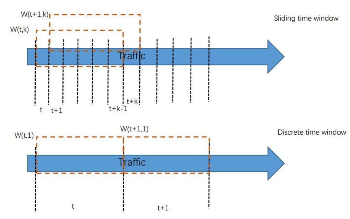
These time slices have the same duration. The length of a time slice could be 1 second, 1 minute or any period in different situations. Every time slice is identified by a number. A sliding time window $W(t,k)$ contains $k$ successive slices starting from the $t$ time slice as shown in the top part of figure 1. Sliding time window will move forward one slice once a time. So two adjacent sliding time windows contain $k-1$ same slices. When $k$ is set to 1, there is no duplicate time period between two adjacent windows, which is the case of discrete time window in the bottom part of figure 1.

Let $A$ be the network from which we want to detect super points. A host’s packets stream in a sliding time window is defined as below.

$aip$’s opposite hosts stream $ST(aip,t,k)$ could be derived from $Pkt(aip,t,k)$ by extracting the other IP address except $aip$. A IP address $bip$ may appear several times in $ST(aip,t,k)$ because $aip$ can send several packets to $bip$ or receive many packets from $bip$. Hosts in $ST(aip,t,k)$ make up of opposite hosts set of $aip$, written as $OP(aip,t,k)$. The number of element in $OP(aip,t,k)$, denoted as $|OP(aip,t,k)|$, is no bigger than that of $ST(aip,t,k)$. $|OP(aip,t,k)|$ is the cardinality of $aip$ in sliding time window $W(t,k)$. Sliding super point is defined according to host’s cardinality.

Threshold $\theta$ is defined by users for different applications. It could be selected according to the average cardinality of all host in the past or the normal cardinality of a server. How to get $|OP(aip,t,k)|$ from $ST(aip,t,k)$ is a hard task. Because packets pass through $ER$ with high speed and every packet could only be scanned a time in the stream. How to process every coming packet, judge if it is a super point and give an accurate estimation of $|OP(aip,t,k)|$ at the end of the last time slice of $W(t,k)$ is the key step in the whole algorithm.

Cardinality estimator scans IP pair stream in a window and gives hosts’ cardinalities estimation at the end of this window. A IP pair is extracted form a packet passing through $R$.

For a host $aip$ in $A$, its IP pair stream $IPpair(aip,t,k)$ is the sub stream of IP pairs which have $aip$ as the first IP addresses. Let $OP(aip,t,k)$ represent the set of the second IP addresses of IP pairs in $IPpair(aip,t,k)$. The task of estimate $aip$’s cardinality is to get the number of hosts in $OP(aip,t,k)$, written as $|OP(aip,t,k)|$, by scanning every IP pair in $IPpair(aip,t,k)$. In order to calculate $|OP(aip,t,k)|$, a key step is to acquire how many distinct IP pairs appear in $W(t,k)$. In another word, for a given IP pair $<aip,bip_{j}>$ which may appears several times in a slice, the problem is to determine if it appears in $W(t,k)$. This problem is simple in discrete time window where $k=1$ by using a single bit which will be set to 1 if $<aip,bip_{j}>$ appears. But in sliding time window when $k>1$, there are $k-1$ slices belong to two adjacent sliding time windows at the same time. For example, when $W(t,k)$ slides to $W(t+1,k)$, there are $k-1$ slices, slice $t+1$ to slice $t+k-1$, appearing in them at the same time. $<aip,bip_{j}>$ may appear in slice $t$ or in some slices after $t$. A sliding cardinality estimator must distinguish these cases and judge if $<aip,bip_{j}>$ appears in the new window after sliding. This paper devises a new recorder, distance recorder $DR$, to solve this problem.

$DR$ is a recorder which consists of $z$ bits. It records the distance between the nearest slice where $<aip,bip_{j}>$ appears and the current scanning slice. For example, suppose that the estimator is now scanning $IPpair(aip,t,k)$ and $<aip,bip_{j}>$ appears in slice $t-d$ and not appears in slices after $t-d$. Then the value of $DR$ is $d$. When $d=0$, the distance will be 0 too which means $<aip,bip_{j}>$ appears in the current slice. Only when the distance is smaller than $k$ will host $bip_{j}$ appears in the sliding time window $W(t,k)$. So $z$ determines the max number of slices in a sliding time window and the max value of $k$ is $2^{z}-1$. In discrete time window, 1 bit is big enough for $DR$. When all of the $z$ bits in $DR$ is set to 1, it means that the distance is more than $k$ and $DR$ is also initialized to this value. $DR$ has four operations as listed below where $dr$, $dr_{1}$, $dr_{2}$ are instance of $DR$.

DRinit($dr$)

set every bit of $dr$ to 1;

DRset($dr$)

set every bit of $dr$ to 0;

DRslide($dr$)

if the value of $dr$ is smaller than $2^{z}-1$, increment $dr$ by 1;

DRjoin($dr_{1}$,$dr_{2}$)

return a new $DR$ which has the max value of $dr_{1}$ and $dr_{2}$

These operations make sure that $DR$ holds the correct distance for a certain IP pair or a certain host in network $B$. A precise way to calculate $|OP(aip,t,k)|$ is to allocate a $DR$ for every host in $OP(aip,t,k)$ and store these $DR$s by hash table or tree structures. This method could acquire the exact value of $|OP(aip,t,k)|$ by counting the number of $DR$ whose value are smaller than $k$ at the end of every slice. But it also consumes many memory and computing resource. For every host in $OP(aip,t,k)$, precise method requires $32+z$ bits, $32$ bits for IP address and $z$ bits for $DR$. The total memory requirement is more than $|OP(aip,t,k)|*(32+z)/8$ bytes. When $|OP(aip,t,k)|$ is very big, locating $DR$ of every host is also a hard task. So precise method is used to run offline to acquire baseline to evaluate the accuracy of other algorithms.

To saving memory and reducing processing time, estimator methods are required. When detection super point, an estimator only needs to tell if a host is super point or not. Under this requirement, a memory efficient algorithm, sliding rough estimator $SRE$, is devised.

For a host $aip$, the task of judging super point is to determine if $|OP(aip,t,k)|\geq\theta$ by scanning every host in $OP(aip,t,k)$ once. $SRE$ proposed in this paper is a memory efficient algorithm which can tell if a host is a super point in a time period with only $g$ $DR$s and 8 $DR$s are big enough for IPv4 address. Its weight $|SRE|^{k}$ is the number of $DR$ in it whose value is smaller than k. These $g$ $DR$s are initialized to $2^{z}-1$ at the begin of a time period. $SRE$ samples and records hosts in $IPpair(aip,t,k)$ by the least significant bits of their hashed value. Least significant bit of an integer is defined in the below.

For example, $LSB(3)=0$, $LSB(40)=3$. The binary formatters of 3 and 40 are “11" and “101000". The first bit of $BIN(3)$ is 1, so $LSB(3)$ equals to 0. While $BIN(40)$ meets its first ‘1’until the fourth bit, so its $LSB$ is 3. For every host $bip$ in $IPpair(aip,t,k)$, $SRE$ hashes it to a random value between 0 and $2^{32}-1$ by a hash function [17] $H_{1}$. If $LSB(H_{1}(bip))$ is smaller than an integer $\tau$, this IP will not be recorded by $SRE$ where $\tau$ is derived from $\theta$ by equation1.

When $LSB(H_{1}(bip))\geq\tau$, a bit selected by $H_{2}(bip)$ will be set where $H_{2}$ is another hash function mapping $bip$ to a value between 0 and $g-1$. After updating a $DR$, if $|SRE|^{k}$ is no smaller than $\rho*g$, $|OP(aip,t,k)|$ is judged as bigger than $\theta$ by $SRE$, where $\rho=0.99*(1-e^{-1/3})$. $\rho$ is acquired from [18]. $SRE$ deals with every host in $IPpair(aip,t,k)$ in this way.

$SRE$ has a high probability to report a super point. Then we will give its mathematical analyze.

$OP(aip,t,k)$ could be regarded as the set of balls and $g$ bits could be regarded as boxes in theorem 1. $|SRE|^{k}$ means the number of $DR$ whose values are smaller than $k$. Suppose there are $\alpha$ hosts in $OP(aip,t,k)$ updating $SRE$. The probability that there are $|SRE|^{k}=g_{1}$ is :

Every host in $OP(aip,t,k)$ has probability $\frac{1}{2^{\tau}}$ to update $SRE$. So the probability that there are $\alpha$ hosts in $OP(aip,t,k)$ updating $SRE$ is:

Combine equation 2 and 3, we will get the probability that there are $g_{1}$ $DR$ being set in $RE$ after scanning $ST(aip,t,k)$ as shown in equation 4.

.

The probability that there are more than $n$ ‘1’ bits in $SRE$ after scanning $ST(aip,t,k)$ could be derived from 4 as shown in equation 5.

Equation 5 proofs that $SRE$ has a high probability to detect super point. But it is a light weight estimator and can’t give an accurate cardinality estimation. Sliding linear estimator introduced in the next makes up this shortage.

Linear estimator, $LE$, is a famous cardinality estimation algorithm[19]. It uses ${g}^{\prime}$ bits, which are initialized to 0 at the beginning of a discrete time window, to estimate host’s cardinality. When scanning a host $bip$ in $IPpair(aip,t,k)$, one bit in $LE$ selected by hash function $H_{3}$ will be set. $H_{3}(bip)$ maps $bip$ to a random value between 0 and ${g}^{\prime}-1$. Let $|LE|$ represent the weight of $LE$, which means the number of 1 bit in it. At the end of a discrete time window, $|OP(aip,t,1)|$ will be estimated by the following equation.

But $LE$ only works when $k=1$. In order to estimate cardinality under sliding time window, sliding linear estimator $SLE$ replaces the ${g}^{\prime}$ bits in $LE$ with ${g}^{\prime}$ $DR$s. The weight of $SLE$ denoted as $|SLE|^{k}$ is the number of short integer whose value is smaller than $k$. $SLE$ estimates a host’s cardinality by equation 7.

According to paper [19], the estimating accuracy of $SLE$ depends on the value of $g^{\prime}$, the bigger $g^{\prime}$ is, the more accurate the estimating result will be. But a big $g^{\prime}$ requires more time to calculating $|SLE|^{k}$ which increasing the estimating time. So $SLE$ is only suit to estimating cardinality of candidate super points at the end of slice, instead of estimating every time while scanning IP pair. When combining $SRE$ with $SLE$, an novel sliding time window super point’s cardinality estimating algorithm $SRLA$ is proposed.

Because 8 $DR$s are big enough for $SRE$ to judge if a host is super point, it can detect super point fast. When using with $LE$, it can estimate super point’s cardinality more quickly. Motivated by this idea, we design a novel estimator, sliding estimator $SE$. $SE$ consists of a $SRE$, a $LE$ and 16 bits. The 16 bits in $SE$ is used to indicate that a host has been judged as a super point in the time slice and we call them as super point indicator $SI$. When a host $aip\in A$ is firstly judged as a super point, a bit in $SI$, selected by a hash function $H_{3}(aip)$ where $H_{3}$ hashes $aip$ to a random value between [0,15], will be set to 1. Let $SI[i]$ point to the $i$th bit in $SI$. An array of $SE$ with $u$ rows and $v$ columns, denoted by $SEA$, is used to detect super points in the network $A$ and estimate their cardinalities. Figure 2 illustrates the structure of $SEA$.

Every IP pair $<aip,bip>$ will update $u$ $SE$ selecting from the $u$ rows of $SEA$ by $u$ hash functions, $RH_{i}(aip)$ where $0\leq i\leq u-1$. $USE(aip)$ represents the union $SE$ of these $u$ $SE$s in $SEA$ and $USI(aip)$, $URE(aip)$ and $ULE(aip)$ represent the $SI$, $SRE$ and $LE$ in $USE(aip)$ respectively. For a host $aip\in A$, its union $SE$ in $SEA$ is acquired by algorithm 1.

$SI[i,j]$, $RE[i,j]$ and $LE[i,j]$ is the $SI$, $SRE$ and $LE$ of $SE$ in the $i$th row, $j$th column. After updating these $SE$s, $aip$ will be checked by $URE(aip)$ to test if it is a super point. If it is and $USI[H_{4}(aip)]$ is zero, $aip$ will be inserted in to a candidate super point list and the $H_{4}(aip)$th bit of every $SI[i,RH_{i}(aip)]$ will be set to 1. This will avoid to add $aip$ to the candidate super point list more times.

To calculate $USE(aip)$ every time scanning an IP pair is time consuming, especially that the $g^{\prime}$ is very big often more than one thousand. We only need to acquire $USI(aip)$ and $URE(aip)$ for super point judging and candidate super point list insertion. $SI$ contains only 16 bits and $SRE$ consists of only 8 $DR$ for IPv4 address. The merging time will be reduced greatly. Algorithm 2 describes how to update $SEA$ for every IP pair.

Algorithm 2 firstly updates $u$ $LE$s by setting a $DR$ of them to 0. Then it begins to update $SRE$ after checking $aip$. Not every IP pair could pass this checking and only about $\frac{1}{2^{\tau}}$ of them updates $SRE$. This checking process accelerates the scanning speed greatly. When a IP pair updates, the first IP address of it will be checked if is a super point by the union $SRE$. Super point reported by $SRE$ will be inserted into the candidate list $CSIP$. Algorithm 2 deals with every IP pair in a slice. After scanning all IP pairs in this slice, the cardinality of hosts in the candidate super point list could be acquired from $SEA$ by the algorithm described in the next section.

$SEA$ uses fix number of $LE$, $u*v$ $SE$s, to estimate the cardinalities of all hosts in $A$. This causes that a $LE$ will record more than one hosts’ cardinalities and the result will be over estimating. In order to reduce the influence, $u$ $LE$s will be used together and a host’s cardinality will be estimated from the union $LE$. But when there are many distinct IP pairs in a slice, there are still many $DR$ in the union $LE$ setting by other hosts. Estimating the number of these error $DR$ and remove them from the union $LE$ helps to improve the accuracy of cardinality estimation.

Let $|LDR(i)|^{k}$ represent the number of all $LE$s’ $DR$ in the $i$th row whose values are smaller than $k$. Then the probability that a $DR$ of a $LE$ in the $i$th row is set by some host is $P_{dr}^{LE}(i)=\frac{|LDR(i)|^{k}}{g^{\prime}*v}$. $|LDR(i)|^{k}$ could be acquired by scanning every $LE$ in the $i$th row. Suppose a $LE$ is used to record the cardinality of a host $aip$ exclusively. Then $|LE|^{k}$ is expected to be $d_{1}=g^{\prime}-g^{\prime}*e^{-\frac{|OP(aip,t,k)|}{g^{\prime}}}$, according to equation 7. In the union $LE$, every of these $d_{1}$ $DR$ will be set by some other hosts with probability $UP_{dr}^{LE}$ as shown in the following equation.

Let $|ULE(aip)|^{k}$ represent the number of $DR$ in the union $LE$ whose values are smaller than $k$. Then $|ULE(aip)|^{k}=d_{1}+(g-d_{1})*UP_{dr}^{LE}$. And $aip$’s cardinality could be estimated by the following equation.

Equation 9 gives a more accurate estimation by removing the error setting $DR$ from $ULE$. The cardinality of every host in the candidate super point list will be estimated in this way.

$SRLA$ works under sliding time window. To do this, $SRLA$ updates $SEA$ incrementally instead of reinitialize it before every time slice. After estimating super point’s cardinality, $SRLA$ updates all $SI$, $DR$ and the candidate super point list by algorithm 3.

Algorithm 3 not only updates all $DR$ in $SEA$ but also derives a new candidate super point list from now current one for the next time window. This makes sure that no super points will be neglected. For example, if $aip$ is a super point in $W(t+1,k)$ and all of its opposite hosts appear in time slice $t+1$ to $t+k-1$. In this case, $aip$ will not be inserted into the candidate super point list while scanning IP pairs in time slice $t+k$. But it could be detected out from the candidate super point lists in $W(t,k)$.

While scanning IP pairs, $SRLA$ only sets some $SI$s, $DR$s. Bot $SI$s and $DR$ could be set by server threads at the same time without causing any mistakes, because a bit or a $DR$ is still being “1" or zero after setting several times. So several IP pairs could be processed concurrently. GPU is a special device which contains plenty computing cores and has high memory accessing through put. Although the ability of every single core of CPU is a little stronger than that of GPU, but the total computing resource of a GPU card is much more abundant than that of CPU considering the plenty number of cores a GPU containing.

GPU is good at these tasks which process huge data with the same instructions. $SRLA$ is such one that scanning different IP pairs by algorithm 2. But GPU could only access its own memory directly, so these IP pairs should be stored in a buffer and then copied to GPU’s graphic memory as shown in figure 3.

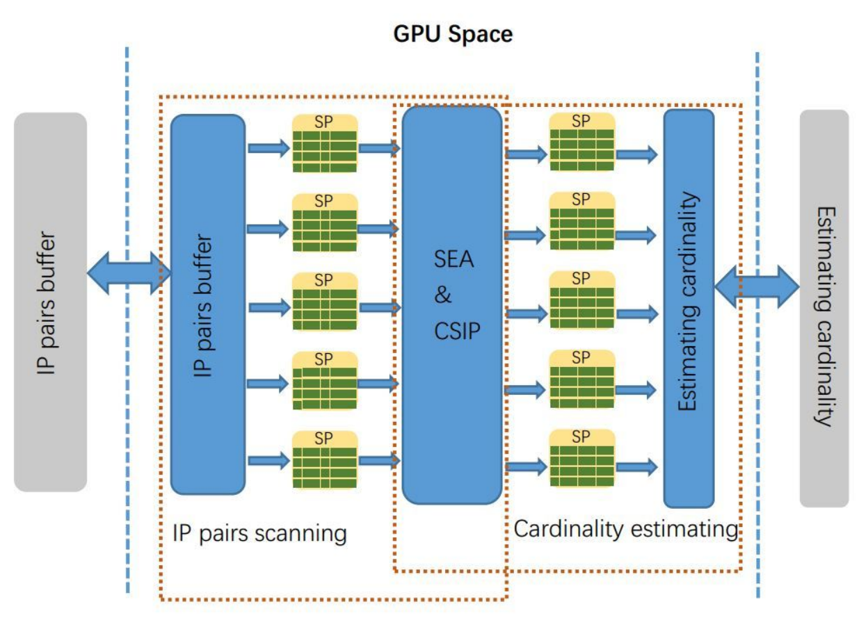
Before $SRLA$ starting, $SEA$ will be initialized on GPU’s graphic memory to be accessed by GPU threads directly. When the IP pairs buffer is full, it will be sent to GPU’s global memory by PCIe bus. After receiving these IP pairs, GPU launches thousands of cores to deal with them at the same time. Stream processor $SP$ is a set of hundreds of computing cores. A GPU card contains several $SP$s. Every $SP$ reads a part of IP pairs in the buffer and distributes them to different cores for further processing. Every core runs algorithm 2 to update $SEA$ and candidate super point list $CSIP$ in a time slice.

After scanning all IP pairs in a slice, every computing core estimates cardinality of candidate super point by equation 9.

Let $C_{u}$ represent the time of IP pairs scanning, $C_{e}$ represent the time of candidate super point’s cardinality estimation and $C_{s}$ represent the duration of a slice. In order to deal with high speed network traffic in real time, $C_{u}+C_{e}$ must be smaller than $C_{s}$. Cardinality of candidate super point will not be estimated until the end of a slice, so the estimating latency under sliding time window is $C_{s}+C_{e}$. Experiments proves that for a 40Gb/s network, $SRLA$’s $C_{e}$ is as small as 300 milliseconds with a common GPU card and $C_{u}$ is smaller than 150 milliseconds. This shows that $SRLA$ works well under a sliding time window whose sliding step could be as small as 1 second when running on GPU.

The parameter of the discrete time window is set to $C_{s}=300$ seconds, $k=1$ and $z=1$. There are 12 discrete time windows in a one-hour traffic and the average information of these two traffics are listed in talbe 1.

In table 1, “$\#ANetIP$" and “$\#BNetIP$" mean the number of hosts in $A$ and $B$ separately and “$\#Flow$" means the average number of distinct IP pairs in a discrete time window. From it we can see that, the average packets speed of this traffic is 4.5 mpps (million packets per second) and super point makes up smaller than 0.047 percent of the total hosts in $A$.

Accuracy is a key merit of cardinality estimation. We measure the accuracy by false positive rate(FPR), false negative rate(FNR) as defined below.

FPR may decrease with the increase of FNR. If an algorithm reports more hosts as super point, its FNR will decrease but FPR will increase. So we use the sum of FPR and FNR, total false rate TFR, to evaluate the accuracy of an algorithm.

The parameters of $SEA$ influences the accuracy of $SRLA$. We firstly compare the accuracy of $SRLA$ with different $u$, $v$ and $g^{\prime}$. Figure 4 and 5 show the average accuracy of $SRLA$ under the 12 discrete time windows of different traffics and parameters.

Every sub figure compares the accuracy of $SRLA$ under different $g^{\prime}$, changing from 1024 to 8192. Big $g^{\prime}$ helps to reduce $TFR$ in most cases. But big $g^{\prime}$ requires more time to acquire $|SLE|^{k}$ which will cause a big $C_{e}$. $TFR$ also decreases gradually with the increase of $v$. But when $v$ grows to 131072 from 65536, $TFR$ decreases slightly but memory doubles. $SRLA$ has the lowest false rate when $g^{\prime}$, $u$ and $v$ are set to the biggest value. But memory requirement and $C_{e}$ also grow rapidly. When $g^{\prime}=1024$, $v=65536$ and $u=4$, $SRLA$’s false rates are small enough and in the following experiments, $SRLA$’s parameters are set as these values. And when running under discrete time window, $z=1$ is enough for $DR$.

To compare the performance of SRLA with other algorithms, we use DCDS[14], VBFA[15], GSE [16] to compare with it. Table 2 lists the average result of all the 24 discrete time windows.

GSE has a lower FPR than other algorithms. It can remove fake super points according the estimating flow number. But GSE may remove some super points too, which causes it has a higher FNR. Because it uses discrete bits to record host’s cardinality, collecting all of these bits together when estimate super points cardinality will use lots of time. DCDS uses CRT when storing host’s cardinality. CRT has a better randomness which makes DCDS has a lower FNR. But CRT is very complex containing many operations. So DCDS’s speed is the lowest among all of these algorithms. VBFA has the fastest speed but its TFR is higher than that of SRLA.

From table 2 we can see that, $SRLA$ uses the smallest memory, smaller than one-twentieth of others’ memory. Because $SRLA$ generates a candidate super point list while packets scanning, so it has the smallest $C_{e}$, only 4 milliseconds. And $SRLA$ is the only one which can run under sliding time window.

In the sliding time window experiments, a time slice is set to 1 second, $k$ is 300 and $z$ equals to 16. We let the window sliding from $W(0,300)$ to $W(2999,300)$ and $SRLA$ runs on traffic 2017-10-21. $SRLA$’s FPR, FNR and TFR are illustrated in figure 6, 7 and 8.

Under most sliding time window, $SRLA$ has a low FNR, smaller than $1.5\%$. When FNR is small, FPR is relative high. But the total false rate is stably small. When under sliding time window, $SRLA$ has the similar accuracy when it under discrete time window. This proves that $SRLA$ estimates super point cardinality successfully under sliding time window on GPU. In the sliding time window experiments, $SRLA$’s average $C_{e}$ is 100 milliseconds which is more than that under discrete time window. Because in sliding time window, $z$ is set to 16 and $SRLA$ requires more time to calculate $|SLE|^{k}$. But $C_{e}+C_{u}$ is still much smaller than $C_{s}$ and $SRLA$’s average $C_{u}$ is 109 milliseconds for every single slice. So $SRLA$ can detect and estimate the cardinality of super point in real time under sliding time window.

References

- [1] S. Khattak, Z. Ahmed, A. A. Syed, and S. A. Khayam, “Botflex: A community-driven tool for botnet detection,” Journal of Network and Computer Applications, vol. 58, pp. 144 – 154, 2015. [Online]. Available: http://www.sciencedirect.com/science/article/pii/S1084804515002155
- [2] G. Kirubavathi and R. Anitha, “Botnet detection via mining of traffic flow characteristics,” Computers Electrical Engineering, vol. 50, pp. 91 – 101, 2016. [Online]. Available: http://www.sciencedirect.com/science/article/pii/S0045790616000148
- [3] H. Khayou and B. Sarakbi, “A validation model for non-lexical routing protocols,” Journal of Network and Computer Applications, vol. 98, pp. 58 – 64, 2017. [Online]. Available: http://www.sciencedirect.com/science/article/pii/S1084804517303028
- [4] Z. Li, W. Liu, Z. Li, and J. Sun, “A bitmap-based algorithm for detecting stealthy superpoints,” in 2014 IEEE 12th International Conference on Dependable, Autonomic and Secure Computing, Aug 2014, pp. 333–337.
- [5] P. Wang, X. Guan, J. Zhao, J. Tao, and T. Qin, “A new sketch method for measuring host connection degree distribution,” IEEE Transactions on Information Forensics and Security, vol. 9, no. 6, pp. 948–960, June 2014.
- [6] J. Cao, Y. Jin, A. Chen, T. Bu, and Z. L. Zhang, “Identifying high cardinality internet hosts,” in IEEE INFOCOM 2009, April 2009, pp. 810–818.
- [7] S. Venkataraman, D. Song, P. B. Gibbons, and A. Blum, “New streaming algorithms for fast detection of superspreaders,” in in Proceedings of Network and Distributed System Security Symposium (NDSS, 2005, pp. 149–166.
- [8] G. Cormode and M. Hadjieleftheriou, “Finding the frequent items in streams of data,” Commun. ACM, vol. 52, no. 10, pp. 97–105, Oct. 2009. [Online]. Available: http://doi.acm.org/10.1145/1562764.1562789
- [9] A. B. Paul, S. Biswas, S. Nandi, and S. Chakraborty, “Matem: A unified framework based on trust and mcdm for assuring security, reliability and qos in dtn routing,” Journal of Network and Computer Applications, vol. 104, pp. 1 – 20, 2018. [Online]. Available: http://www.sciencedirect.com/science/article/pii/S1084804517304010
- [10] M. Bahnasy, H. Elbiaze, and B. Boughzala, “Zero-queue ethernet congestion control protocol based on available bandwidth estimation,” Journal of Network and Computer Applications, vol. 105, pp. 1 – 20, 2018. [Online]. Available: http://www.sciencedirect.com/science/article/pii/S108480451730423X
- [11] A. C谩novas, M. Taha, J. Lloret, and J. Tom谩s, “Smart resource allocation for improving qoe in ip multimedia subsystems,” Journal of Network and Computer Applications, vol. 104, pp. 107 – 116, 2018. [Online]. Available: http://www.sciencedirect.com/science/article/pii/S1084804517304277
- [12] R. Masoudi and A. Ghaffari, “Software defined networks: A survey,” Journal of Network and Computer Applications, vol. 67, pp. 1 – 25, 2016. [Online]. Available: http://www.sciencedirect.com/science/article/pii/S1084804516300297
- [13] C. Estan, G. Varghese, and M. Fisk, “Bitmap algorithms for counting active flows on high-speed links,” IEEE/ACM Trans. Netw., vol. 14, no. 5, pp. 925–937, Oct. 2006. [Online]. Available: http://dx.doi.org/10.1109/TNET.2006.882836
- [14] P. Wang, X. Guan, T. Qin, and Q. Huang, “A data streaming method for monitoring host connection degrees of high-speed links,” IEEE Transactions on Information Forensics and Security, vol. 6, no. 3, pp. 1086–1098, Sept 2011.
- [15] W. Liu, W. Qu, J. Gong, and K. Li, “Detection of superpoints using a vector bloom filter,” IEEE Transactions on Information Forensics and Security, vol. 11, no. 3, pp. 514–527, March 2016.
- [16] S.-H. Shin, E.-J. Im, and M. Yoon, “A grand spread estimator using a graphics processing unit,” Journal of Parallel and Distributed Computing, vol. 74, no. 2, pp. 2039 – 2047, 2014. [Online]. Available: http://www.sciencedirect.com/science/article/pii/S0743731513002189
- [17] P. Indyk, “A small approximately min-wise independent family of hash functions,” Journal of Algorithms, vol. 38, no. 1, pp. 84 – 90, 2001. [Online]. Available: http://www.sciencedirect.com/science/article/pii/S0196677400911313
- [18] D. M. Kane, J. Nelson, and D. P. Woodruff, “An optimal algorithm for the distinct elements problem,” in Proceedings of the Twenty-ninth ACM SIGMOD-SIGACT-SIGART Symposium on Principles of Database Systems, ser. PODS ’10. New York, NY, USA: ACM, 2010, pp. 41–52. [Online]. Available: http://doi.acm.org/10.1145/1807085.1807094
- [19] K.-Y. Whang, B. T. Vander-Zanden, and H. M. Taylor, “A linear-time probabilistic counting algorithm for database applications,” ACM Trans. Database Syst., vol. 15, no. 2, pp. 208–229, Jun. 1990. [Online]. Available: http://doi.acm.org/10.1145/78922.78925
- [20] CERNET, “China education and research network,” http://iptas.edu.cn/src/system.php, 2017, online;accessed 2017.