跳到论文正文
W Papers独立论文阅读器 arXiv:1803.10359 论文正文 计算阅读时间 · 0%
引用这篇论文根据当前论文元数据生成,正式投稿前建议核对。


License: arXiv.org perpetual non-exclusive license
arXiv:1803.10359v4 [math.OC] 11 Sep 2019

Achieving Linear Convergence in Distributed Asynchronous Multi-agent Optimization

Ye Tian    Ying Sun    Gesualdo Scutari ††thanks: Part of this work has been presented at the 56th Annual Allerton Conference [1] and posted on arxiv [2] on March 2018. This work has been supported by the USA National Science Foundation under Grants CIF 1632599 and CIF 1719205; and in part by the Office of Naval Research under Grant N00014-16-1-2244, and the Army Research Office under Grant W911NF1810238.††thanks: The authors are with the School of Industrial Engineering, Purdue University, West-Lafayette, IN, USA; Emails: {tian110,sun578,gscutari}@purdue.edu.
Abstract

This papers studies multi-agent (convex and nonconvex) optimization over static digraphs. We propose a general distributed asynchronous algorithmic framework whereby i) agents can update their local variables as well as communicate with their neighbors at any time, without any form of coordination; and ii) they can perform their local computations using (possibly) delayed, out-of-sync information from the other agents. Delays need not be known to the agent or obey any specific profile, and can also be time-varying (but bounded). The algorithm builds on a tracking mechanism that is robust against asynchrony (in the above sense), whose goal is to estimate locally the average of agents’ gradients. When applied to strongly convex functions, we prove that it converges at an R-linear (geometric) rate as long as the step-size is sufficiently small. A sublinear convergence rate is proved, when nonconvex problems and/or diminishing, uncoordinated step-sizes are considered. To the best of our knowledge, this is the first distributed algorithm with provable geometric convergence rate in such a general asynchronous setting. Preliminary numerical results demonstrate the efficacy of the proposed algorithm and validate our theoretical findings.

Index Terms:
Asynchrony, Delay, Directed graphs, Distributed optimization, Linear convergence, Nonconvex optimization.

I Introduction

We study convex and nonconvex distributed optimization over a network of agents, modeled as a directed fixed graph. Agents aim at cooperatively solving the optimization problem

min𝐱∈ℝn⁡F⁡(𝐱)≜∑i=1Ifi​(𝐱)\min_{\mathbf{x}\in\mathbb{R}^{n}}F(\mathbf{x})\triangleq\sum_{i=1}^{I}f_{i}\big(\mathbf{x}\big)\vskip-2.84544pt (P)

where fi:n→f_{i}:\real^{n}\rightarrow\real is the cost function of agent ii, assumed to be smooth (nonconvex) and known only to agent ii. In this setting, optimization has to be performed in a distributed, collaborative manner: agents can only receive/send information from/to its immediate neighbors. Instances of (P) that require distributed computing have found a wide range of applications in different areas, including network information processing, resource allocation in communication networks, swarm robotic, and machine learning, just to name a few.

Many of the aforementioned applications give rise to extremely large-scale problems and networks, which naturally call for asynchronous, parallel solution methods. In fact, asynchronous modus operandi reduces the idle times of workers, mitigate communication and/or memory-access congestion, save power (as agents need not perform computations and communications at every iteration), and make algorithms more fault-tolerant. In this paper, we consider the following very general, abstract, asynchronous model [3]:

(i)

Agents can perform their local computations as well as communicate (possibly in parallel) with their immediate neighbors at any time, without any form of coordination or centralized scheduling; and

(ii)

when solving their local subproblems, agents can use outdated information from their neighbors.

In (ii) no constraint is imposed on the delay profiles: delays can be arbitrary (but bounded), time-varying, and (possibly) dependent on the specific activation rules adopted to wakeup the agents in the network. This model captures in a unified fashion several forms of asynchrony: some agents execute more iterations than others; some agents communicate more frequently than others; and inter-agent communications can be unreliable and/or subject to unpredictable, time-varying delays.

Several forms of asynchrony have been studied in the literature–see Sec. I-A for an overview of related works. However, we are not aware of any distributed algorithm that is compliant to the asynchrony model (i)-(ii) and distributed (nonconvex) setting above. Furthermore, when considering the special case of a strongly convex function FF, it is not clear how to design a (first-order) distributed asynchronous algorithm (as specified above) that achieves linear convergence rate. This paper answers these questions–see Sec. I-B and Table 1 for a summary of our contributions.

Algorithm Nonconvex Cost Function No Idle Time Arbitrary Delays Parallel Step Sizes Digraph Global Convergence to Exact Solutions Rate Analysis
Fixed Uncoordinated Diminishing Linear Rate for Strongly Convex Nonconvex
Asyn. Broadcast [4] ✓ ✓ ✓ In expectation (w. diminishing step)
Asyn. Diffusion [5] ✓
Asyn. ADMM [6] ✓ ✓ Deterministic
Dual Ascent in [7] ✓ Restricted Restricted ✓
ra-NRC [8] ✓ ✓
ARock [9] ✓ Restricted ✓ Almost surely In expectation
ASY-PrimalDual [10] ✓ Restricted ✓ Almost surely
ASY-SONATA ✓ ✓ ✓ ✓ ✓ ✓ ✓ Deterministic Deterministic Deterministic
Table 1: Comparison with state-of-art distributed asynchronous algorithms. Current schemes can deal with uncoordinated activations but only with some forms of delays. ASY-SONATA enjoys all the desirable features listed in the table.

I-A Literature Review

Since the seminal work [11], asynchronous parallelism has been applied to several centralized optimization algorithms, including block coordinate descent (e.g., [11, 12, 13]) and stochastic gradient (e.g., [14, 15]) methods. However, these schemes are not applicable to the networked setup considered in this paper, because they would require the knowledge of the function FF from each agent. Distributed methods exploring (some form of) asynchrony over networks with no centralized node have been studied in [16, 17, 18, 19, 20, 21, 22, 23, 24, 25, 26, 4, 5, 6, 7, 8, 9, 10]. We group next these works based upon the features (i)-(ii) above.

(a) Random activations and no delays [16, 17, 18, 19, 20]: These schemes considered distributed convex unconstrained optimization over undirected graphs. While substantially different in the form of the updates performed by the agents–[16, 18, 20] are instances of primal-dual (proximal-based) algorithms, [19] is an ADMM-type algorithm, while [17] is based on the distributed gradient tracking mechanism introduced in[27, 28, 29]–all these algorithms are asynchronous in the sense of feature (i) [but not (ii)]: at each iteration, a subset of agents [16, 18, 20] (or edge-connected agents [19, 17]), chosen at random, is activated, performing then their updates and communications with their immediate neighbors; between two activations, agents are assumed to be in idle mode (i.e., able to continuously receive information). However, no form of delays is allowed: every agent must perform its local computations/updates using the most updated information from its neighbors. This means that all the actions performed by the agent(s) in an activation must be completed before a new activation (agent) takes place (wakes-up), which calls for some coordination among the agents. Finally, no convergence rate was provided for the aforementioned schemes but [19, 17].
(b) Synchronous activations and delays [21, 22, 23, 24, 25, 26]: These schemes considered distributed constrained convex optimization over undirected graphs. They study the impact of delayed gradient information [21, 22] or communication delays (fixed [23], uniform [26, 22] or time-varying [24, 25]) on the convergence rate of distributed gradient (proximal [21, 22] or projection-based [25, 26]) algorithms or dual-averaging distributed-based schemes [23, 24]. While these schemes are all synchronous [thus lacking of feature (i)], they can tolerate communication delays [an instantiation of feature (ii)], converging at a sublinear rate to an optimal solution. Delays must be such that no losses occur–every agent’s message will eventually reach its destination within a finite time.
(c) Random/cyclic activations and some form of delays [4, 5, 6, 7, 8, 9, 10]: The class of optimization problems along with the key features of the algorithms proposed in these papers are summarized in Table 1 and briefly discussed next. The majority of these works studied distributed (strongly) convex optimization over undirected graphs, with [5] assuming that all the functions fif_{i} have the same minimizer, [6] considering also nonconvex objectives, and [8] being implementable also over digraphs. The algorithms in [4, 5] are gradient-based schemes; [6] is a decentralized instance of ADMM; [9] applies an asynchronous parallel ADMM scheme to distributed optimization; and [10] builds on a primal-dual method. The schemes in [7, 8] instead build on (approximate) second-order information. All these algorithms are asynchronous in the sense of feature (i): [4, 5, 6, 9, 10] considered random activations of the agents (or edges-connected agents) while [7, 8] studied deterministic, uncoordinated activation rules. As far as feature (ii) is concerned, some form of delays is allowed. More specifically, [4, 5, 6, 8] can deal with packet losses: the information sent by an agent to its neighbors either gets lost or received with no delay. They also assume that agents are always in idle mode between two activations. Closer to the proposed asynchronous framework are the schemes in [9, 10] wherein a probabilistic model is employed to describe the activation of the agents and the aged information used in their updates. The model requires that the random variables triggering the activation of the agents are i.i.d and independent of the delay vector used by the agent to performs its update. While this assumption makes the convergence analysis possible, in reality, there is a strong dependence of the delays on the activation index; see [13] for a detailed discussion on this issue and several counter examples. Other consequences of this model are: the schemes [9, 10] are not parallel–only one agent per time can perform the update–and a random self-delay must be used in the update of each agent (even if agents have access to their most recent information). Furthermore, [9] calls for the solution of a convex subproblem for each agent at every iteration. Referring to the convergence rate, [9] is the only scheme exhibiting linear convergence in expectation, when each fif_{i} is strongly convex and the graph undirected. No convergence rate is available in any of the aforementioned papers, when FF is nonconvex.

I-B Summary of Contributions

This paper proposes a general distributed, asynchronous algorithmic framework for (strongly) convex and nonconvex instances of Problem (P), over directed graphs. The algorithm leverages a perturbed “sum-push” mechanism that is robust against asynchrony, whose goal is to track locally the average of agents’ gradients; this scheme along with its convergence analysis are of independent interest. To the best of our knowledge, the proposed framework is the first scheme combining the following attractive features (cf. Table 1): (a) it is parallel and asynchronous [in the sense (i) and (ii)]–multiple agents can be activated at the same time (with no coordination) and/or outdated information can be used in the agents’ updates; our asynchronous setting (i) and (ii) is less restrictive than the one in [9, 10]; furthermore, in contrast with [9], our scheme avoids solving possibly complicated subproblems; (b) it is applicable to nonconvex problems, with probable convergence to stationary solutions of (P); (c) it is implementable over digraph; (d) it employs either a constant step-size or uncoordinated diminishing ones; (e) it converges at an R-linear rate (resp. sublinear) when FF is strongly convex (resp. nonconvex) and a constant (resp. diminishing, uncoordinated) step-size(s) is employed; this contrasts [9] wherein each fif_{i} needs to be strongly convex; and (f) it is “protocol-free”, meaning that agents need not obey any specific communication protocols or asynchronous modus operandi (as long as delays are bounded and agents update/communicate uniformly infinitely often).

On the technical side, convergence is studied introducing two techniques of independent interest, namely: i) the asynchronous agent system is reduced to a synchronous “augmented” one with no delays by adding virtual agents to the graph. While this idea was first explored in [30, 31],[32], the proposed enlarged system and algorithm differ from those used therein, which cannot deal with the general asynchronous model considered here–see Remark 13, Sec.VI; and ii) the rate analysis is employed putting forth a generalization of the small gain theorem (widely used in the literature [33] to analyze synchronous schemes), which is expected to be broadly applicable to other distributed algorithms.

I-C Notation

Throughout the paper we use the following notation. Given the matrix 𝐌≜(Mi​j)i,j=1I\mathbf{M}\triangleq(M_{ij})_{i,j=1}^{I}, 𝐌i,:\mathbf{M}_{i,:} and 𝐌:,j\mathbf{M}_{:,j} denote its ii-th row vector and jj-th column vector. Given the sequence {𝐌t}t=sk\{\mathbf{M}^{t}\}_{t=s}^{k}, with k≥sk\geq s, we define 𝐌k:s≜𝐌k𝐌k−1⋯𝐌s+1𝐌s\mathbf{M}^{k:s}\triangleq\mathbf{M}^{k}\mathbf{M}^{k-1}\cdots\mathbf{M}^{s+1}\mathbf{M}^{s}, if k>sk>s; and 𝐌k:s≜𝐌s\mathbf{M}^{k:s}\triangleq\mathbf{M}^{s} otherwise. Given two matrices (vectors) 𝐀\mathbf{A} and 𝐁\mathbf{B} of same size, by 𝐀≼𝐁\mathbf{A}\preccurlyeq\mathbf{B} we mean that 𝐁−𝐀\mathbf{B}-\mathbf{A} is a nonnegative matrix (vector). The dimensions of the all-one vector 𝟏\mathbf{1} and the ii-th canonical vector 𝐞i\mathbf{e}_{i} will be clear from the context. We use ‖⋅‖\left\lVert\cdot\right\rVert to represent the Euclidean norm for a vector whereas the spectral norm for a matrix. The indicator function 𝟙​[E]\mathbbm{1}[E] of an event EE equals to 11 when the event EE is true, and 00 otherwise. Finally, we use the convention ∑t∈∅xt=0\sum_{t\in\emptyset}x^{t}=0 and ∏t∈∅xt=1\prod_{t\in\emptyset}x^{t}=1.

II Problem Setup and Preliminaries

II-A Problem Setup

We study Problem (P) under the following assumptions.

Assumption 1 (On the optimization problem).

  1. a.

    Each fi:ℝn→ℝf_{i}:\mathbb{R}^{n}\rightarrow\mathbb{R} is proper, closed and LiL_{i}-Lipschitz differentiable;

  2. b.

    FF is bounded from below. □\square

Note that fif_{i} need not be convex. We also make the blanket assumption that each agent ii knows only its own fif_{i}, but not ∑j≠ifj\sum_{j\neq i}f_{j}. To state linear convergence, we will use the following extra condition on the objective function.

Assumption 2 (Strong convexity).

Assumption 1(i) holds and, in addition, FF is τ\tau-strongly convex. □\square

On the communication network: The communication network of the agents is modeled as a fixed, directed graph 𝒢=(𝒱,ℰ)\mathcal{G}=(\mathcal{V},\mathcal{E}), where 𝒱={1,…,I}\mathcal{V}=\{1,\ldots,I\} is the set of nodes (agents), and ℰ⊆𝒱×𝒱\mathcal{E}\subseteq\mathcal{V}\times\mathcal{V} is the set of edges (communication links). If (i,j)∈ℰ(i,j)\in\mathcal{E}, it means that agent ii can send information to agent jj. We assume that the digraph does not have self-loops. We denote by 𝒩iin\mathcal{N}_{i}^{\text{in}} the set of in-neighbors of node ii, i.e., 𝒩iin≜{j∈𝒱∣(j,i)∈ℰ}\mathcal{N}_{i}^{\text{in}}\triangleq\left\{j\in\mathcal{V}\mid(j,i)\in\mathcal{E}\right\} while 𝒩iout≜{j∈𝒱∣(i,j)∈ℰ}\mathcal{N}_{i}^{\text{out}}\triangleq\left\{j\in\mathcal{V}\mid(i,j)\in\mathcal{E}\right\} is the set of out-neighbors of agent ii. We make the following standard assumption on the graph connectivity.

Assumption 3.

The graph 𝒢\mathcal{G} is strongly connected. □\square

II-B Preliminaries: The SONATA algorithm [34, 35]

The proposed asynchronous algorithmic framework builds on the synchronous SONATA algorithm, proposed in [34, 35] to solve (nonconvex) multi-agent optimization problems over time-varying digraphs. This is motivated by the fact that SONATA has the unique property of being provably applicable to both convex and nonconvex problems, and it achieves linear convergence when applied to strongly convex objectives FF. We thus begin reviewing SONATA, tailored to (P); then we generalized it to the asynchronous setting (cf. Sec. IV).

Every agent controls and iteratively updates the tuple (𝐱i,𝐲i,𝐳i,ϕi)(\mathbf{x}_{i},\mathbf{y}_{i},{\mathbf{z}_{i}},\phi_{i}): 𝐱i\mathbf{x}_{i} is agent ii’s copy of the shared variables 𝐱\mathbf{x} in (P); 𝐲i\mathbf{y}_{i} acts as a local proxy of the sum-gradient ∇F\nabla F; and 𝐳i\mathbf{z}_{i} and ϕi\phi_{i} are auxiliary variables instrumental to deal with communications over digraphs. Let 𝐱ik,𝐳ik\mathbf{x}_{i}^{k},\mathbf{z}_{i}^{k}, ϕik\phi_{i}^{k}, and 𝐲ik\mathbf{y}_{i}^{k} denote the value of the aforementioned variables at iteration k∈ℕ0k\in\mathbb{N}_{0}. The update of each agent ii reads:

𝐱ik+1\displaystyle\mathbf{x}_{i}^{k+1} =∑j∈𝒩iin∪{i}wi​j​(𝐱jk−αk​𝐲jk),\displaystyle=\sum_{j\in\mathcal{N}_{i}^{\text{in}}\cup\{i\}}w_{ij}\,{{{\left(\mathbf{x}_{j}^{k}-\alpha^{k}\,\mathbf{y}_{j}^{k}\right)}}}, (1)
𝐳ik+1\displaystyle\mathbf{z}_{i}^{k+1} =∑j∈𝒩iin∪{i}ai​j​𝐳jk+∇fi​(𝐱ik+1)−∇fi​(𝐱ik),\displaystyle=\sum_{j\in\mathcal{N}_{i}^{\text{in}}\cup\{i\}}a_{ij}\mathbf{z}_{j}^{k}+\nabla f_{i}(\mathbf{x}_{i}^{k+1})-\nabla f_{i}(\mathbf{x}_{i}^{k}), (2)
ϕik+1\displaystyle\phi_{i}^{k+1} =∑j∈𝒩iin∪{i}ai​j​ϕjk,\displaystyle=\sum_{j\in\mathcal{N}_{i}^{\text{in}}\cup\{i\}}a_{ij}\phi_{j}^{k}, (3)
𝐲ik+1\displaystyle\mathbf{y}_{i}^{k+1} =𝐳ik+1/ϕik+1,\displaystyle=\mathbf{z}_{i}^{k+1}/\phi_{i}^{k+1}, (4)

with 𝐳i0=𝐲i0=∇fi​(𝐱i0)\mathbf{z}_{i}^{0}=\mathbf{y}_{i}^{0}=\nabla f_{i}(\mathbf{x}_{i}^{0}) and ϕi0=1\phi_{i}^{0}=1, for all i∈𝒱i\in\mathcal{V}. In (1), 𝐲ik\mathbf{y}_{i}^{k} is a local estimate of the average-gradient (1/I)​∑i=1I∇fi​(𝐱ik)({1}/{I})\sum_{i=1}^{I}\nabla f_{i}(\mathbf{x}_{i}^{k}). Therefore, every agent, first moves along the estimated gradient direction, generating 𝐱ik−αk​𝐲ik\mathbf{x}_{i}^{k}-\alpha^{k}\,\mathbf{y}_{i}^{k} (αk\alpha^{k} is the step-size); and then performs a consensus step to force asymptotic agreement among the local variables 𝐱i\mathbf{x}_{i}. Steps (2)-(4) represent a perturbed-push-sum update, aiming at tracking the gradient (1/I)∇F({1}/{I})\,\nabla F [29, 35, 28]. The weight-matrices 𝐖≜(wi​j)i,j=1I\mathbf{W}\triangleq(w_{ij})_{i,j=1}^{I} and 𝐀≜(ai​j)i,j=1I\mathbf{A}\triangleq(a_{ij})_{i,j=1}^{I} satisfy the following standard assumptions.

Assumption 4 (On the weight-matrices).

The weight-matrices 𝐖≜(wi​j)i,j=1I\mathbf{W}\triangleq(w_{ij})_{i,j=1}^{I} and 𝐀≜(ai​j)i,j=1I\mathbf{A}\triangleq(a_{ij})_{i,j=1}^{I} satisfy (we will write 𝐌≜(mi​j)i,j=1I\mathbf{M}\triangleq(m_{ij})_{i,j=1}^{I} to denote either 𝐀\mathbf{A} or 𝐖\mathbf{W}):

  1. a.

    ∃m¯>0\exists\,\bar{m}>0 such that mi​i≥m¯m_{ii}\geq\bar{m}, for all i∈𝒱i\in\mathcal{V}; and mi​j≥m¯m_{ij}\geq\bar{m}, for all (j,i)∈ℰ(j,i)\in\mathcal{E}; mi​j=0m_{ij}=0, otherwise;

  2. b.

    𝐖\mathbf{W} is row-stochastic, that is, 𝐖​ 1=𝟏\mathbf{W}\,\mathbf{1}=\mathbf{1};

  3. c.

    𝐀\mathbf{A} is column-stochastic, that is, 𝐀T​ 1=𝟏\mathbf{A}^{T}\,\mathbf{1}=\mathbf{1}; □\square

In [33], a special instance of SONATA, was proved to converges at an R-linear rate when FF is strongly convex. This result was extended to constrained, nonsmooth (composite), distributed optimization in [36]. A natural question is whether SONATA works also in an asynchronous setting still converging at a linear rate. Naive asynchronization of the updates (1)-(4)–such as using uncoordinated activations and/or replacing instantaneous information with a delayed one–would not work. For instance, the tracking (2)-(4) calls for the invariance of the averages, i.e., ∑i=1I𝐳ik=∑i=1I∇fi​(𝐱k)\sum_{i=1}^{I}\mathbf{z}^{k}_{i}=\sum_{i=1}^{I}\nabla f_{i}(\mathbf{x}^{k}), for all k∈ℕ0k\in\mathbb{N}_{0}. It is not difficult to check that any perturbation in (2)-e.g., in the form of delays or packet losses–puts in jeopardy this property.

To cope with the above challenges, a first step is robustifying the gradient tracking scheme. In Sec. III, we introduce P-ASY-SUM-PUSH–an asynchronous, perturbed, instance of the push-sum algorithm [37], which serves as a unified algorithmic framework to accomplish several tasks over digraphs in an asynchronous manner, such as solving the average consensus problem and tracking the average of agents’ time-varying signals. Building on P-ASY-SUM-PUSH, in Sec. IV, we finally present the proposed distributed asynchronous optimization framework, termed ASY-SONATA.

III Perturbed Asynchronous Sum-Push

We present P-ASY-SUM-PUSH; the algorithm was first introduced in our conference paper [1], which we refer to for details on the genesis of the scheme and intuitions; here we directly introduce the scheme and study its convergence.
Consider an asynchronous setting wherein agents compute and communicate independently without coordination. Every agent ii maintains state variables 𝐳i\mathbf{z}_{i}, ϕi\phi_{i}, 𝐲i\mathbf{y}_{i}, along with the following auxiliary variables that are instrumental to deal with uncoordinated activations and delayed information: i) the cumulative-mass variables 𝝆j​i\bm{\rho}_{ji} and σj​i\sigma_{ji}, with j∈𝒩ioutj\in\mathcal{N}_{i}^{\text{out}}, which capture the cumulative (sum) information generated by agent ii up to the current time and to be sent to agent j∈𝒩ioutj\in\mathcal{N}_{i}^{\text{out}}; consequently, 𝝆i​j\bm{\rho}_{ij} and σi​j\sigma_{ij} are received by ii from its in-neighbors j∈𝒩iinj\in\mathcal{N}_{i}^{\text{in}}; and ii) the buffer variables 𝝆~i​j\tilde{\bm{\rho}}_{ij} and σ~i​j\tilde{\sigma}_{ij}, with j∈𝒩iinj\in\mathcal{N}_{i}^{\text{in}}, which store the information sent from j∈𝒩iinj\in\mathcal{N}_{i}^{\text{in}} to ii and used by ii in its last update. Values of these variables at iteration k∈ℕ0k\in\mathbb{N}_{0} are denoted by the same symbols with the superscript “kk”. Note that, because of the asynchrony, each agent ii might have outdated 𝝆i​j\bm{\rho}_{ij} and σi​j\sigma_{ij}; 𝝆i​jk−djk\bm{\rho}_{ij}^{k-d_{j}^{k}} (resp. σi​jk−djk\sigma_{ij}^{k-d_{j}^{k}}) is a delayed version of the current 𝝆i​jk\bm{\rho}_{ij}^{k} (resp. σi​jk\sigma_{ij}^{k}) owned by jj at time kk, where 0≤djk≤D<∞0\leq d_{j}^{k}\leq D<\infty is the delay. Similarly, 𝝆~i​j\tilde{\bm{\rho}}_{ij} and σ~i​j\tilde{\sigma}_{ij} might differ from the last information generated by jj for ii, because agent ii might not have received that information yet (due to delays) or never will (due to packet losses).
The proposed asynchronous algorithm, P-ASY-SUM-PUSH, is summarized in Algorithm 1. A global iteration clock (not known to the agents) is introduced: k→k+1k\to k+1 is triggered based upon the completion from one agent, say iki^{k}, of the following actions. (S.2): agent iki^{k} maintains a local variable τik​j\tau_{i^{k}j}, for each j∈𝒩ikinj\in\mathcal{N}_{i^{k}}^{\text{in}}, which keeps track of the “age” (generated time) of the (𝝆,σ)({\bm{\rho}},\sigma)-variables that it has received from its in-neighbors and already used. If k−djkk-d_{j}^{k} is larger than the current counter τik​jk−1\tau_{i^{k}j}^{k-1}, indicating that the received (𝝆,σ)({\bm{\rho}},\sigma)-variables are newer than those currently stored, agent iki^{k} accepts 𝝆ik​jk−djk{\bm{\rho}}_{i^{k}j}^{k-d_{j}^{k}} and σik​jk−djk{\sigma}_{i^{k}j}^{k-d_{j}^{k}}, and updates τik​j\tau_{i^{k}j} as k−djkk-d_{j}^{k}; otherwise, the variables will be discarded and τik​j\tau_{i^{k}j} remains unchanged. Note that (5) can be performed without any coordination. It is sufficient that each agent attaches a time-stamp to its produced information reflecting it local timing counter. We describe next the other steps, assuming that new information has come in to agent iki^{k}, that is, τik​j=k−djk\tau_{i^{k}j}=k-d_{j}^{k}.

Algorithm 1 P-ASY-SUM-PUSH (Global View)
Data: 𝐳i0∈ℝn\mathbf{z}_{i}^{0}\in\mathbb{R}^{n}, ϕi0=1\phi_{i}^{0}=1, 𝝆~i​j0=0\tilde{\bm{\rho}}_{ij}^{0}=0, σ~i​j0=0\tilde{\sigma}_{ij}^{0}=0, τi​j−1=−D\tau_{ij}^{-1}=-D, for all j∈𝒩iinj\in\mathcal{N}_{i}^{\text{in}} and i∈𝒱i\in\mathcal{V}; σi​jt=0\sigma_{ij}^{t}=0 and 𝝆i​jt=0\bm{\rho}_{ij}^{t}=0, for all t=−D,…,0t=-D,\ldots,0; and {ϵk}k∈ℕ0\{{\bm{\epsilon}}^{k}\}_{k\in\mathbb{N}_{0}}. Set k=0k=0.
While: a termination criterion is not met do
  (S.1) Pick (ik,𝐝k)(i^{k},\mathbf{d}^{k}), with 𝐝k≜(djk)j∈𝒩ikin\mathbf{d}^{k}\triangleq(d_{j}^{k})_{j\in\mathcal{N}_{{i}^{k}}^{\text{in}}};
  (S.2) Set (purge out the old information):
τik​jk=max⁡(τik​jk−1,k−djk),∀j∈𝒩ikin;\displaystyle\tau_{i^{k}j}^{k}=\max\big(\tau_{i^{k}j}^{k-1},k-d_{j}^{k}\big),\quad\forall j\in\mathcal{N}_{i^{k}}^{\text{in}}; (5)
  (S.3) Update the variables performing
  • •

    (S.3.1) Sum step:

    𝐳ikk+12=𝐳ikk+∑j∈𝒩ikin(𝝆ik​jτik​jk−𝝆~ik​jk)+ϵk\displaystyle\mathbf{z}_{i^{k}}^{k+\frac{1}{2}}=\mathbf{z}_{i^{k}}^{k}+\displaystyle\sum_{j\in\mathcal{N}_{i^{k}}^{\text{in}}}\left({\bm{\rho}}_{{i^{k}}j}^{\tau_{i^{k}j}^{k}}-\tilde{\bm{\rho}}_{i^{k}j}^{k}\right)+\bm{\epsilon}^{k} (6)
    ϕikk+12=ϕikk+∑j∈𝒩ikin(σik​jτik​jk−σ~ik​jk)\displaystyle\phi_{i^{k}}^{k+\frac{1}{2}}=\phi_{i^{k}}^{k}+\displaystyle\sum_{j\in\mathcal{N}_{i^{k}}^{\text{in}}}\left({\sigma}_{{i^{k}}j}^{\tau_{i^{k}j}^{k}}-\tilde{\sigma}_{i^{k}j}^{k}\right)
  • •

    (S.3.2) Push step:

    𝐳ikk+1=aik​ik​𝐳ikk+12,ϕikk+1=aik​ik​ϕikk+12\displaystyle\mathbf{z}_{i^{k}}^{k+1}=a_{i^{k}i^{k}}\,\mathbf{z}_{i^{k}}^{k+\frac{1}{2}},\hskip 9.24994pt\phi_{i^{k}}^{k+1}=a_{i^{k}i^{k}}\,\phi_{i^{k}}^{k+\frac{1}{2}}
    𝝆j​ikk+1=𝝆j​ikk+aj​ik​𝐳ikk+12,\displaystyle{\bm{\rho}}_{j{i^{k}}}^{k+1}={\bm{\rho}}_{j{i^{k}}}^{k}+a_{j{i^{k}}}\,\mathbf{z}_{i^{k}}^{k+\frac{1}{2}}, (7)
    σj​ikk+1=σj​ikk+aj​ik​ϕikk+12,∀j∈𝒩ikout\displaystyle{\sigma}_{j{i^{k}}}^{k+1}={\sigma}_{j{i^{k}}}^{k}+a_{j{i^{k}}}\,\phi_{i^{k}}^{k+\frac{1}{2}},\hskip 9.24994pt\forall j\in\mathcal{N}_{i^{k}}^{\text{out}}
  • •

    (S.3.3) Mass-Buffer update:

    𝝆~ik​jk+1=𝝆ik​jτik​jk,σ~ik​jk+1=σik​jτik​jk,∀j∈𝒩ikin\displaystyle\tilde{\bm{\rho}}_{{i^{k}}j}^{k+1}={\bm{\rho}}_{{i^{k}}j}^{\tau_{i^{k}j}^{k}},\hskip 9.24994pt\tilde{\sigma}_{{i^{k}}j}^{k+1}={\sigma}_{{i^{k}}j}^{\tau_{i^{k}j}^{k}},{\hskip 9.24994pt\,\ \forall j\in\mathcal{N}_{i^{k}}^{\text{in}}} (8)
  • •

    (S.3.4) Set: 𝐲ikk+1=𝐳ikk+1/ϕikk+1.\hskip 9.24994pt\mathbf{y}_{i^{k}}^{k+1}=\mathbf{z}_{i^{k}}^{k+1}/\phi_{i^{k}}^{k+1}.

  (S.4) Untouched state variables shift to state k+1k+1 while keeping the same value; k←k+1k\leftarrow k+1.

(S.3.1): In (6), agent iki^{k} builds the intermediate “mass” 𝐳ikk+12\mathbf{z}_{i^{k}}^{k+\frac{1}{2}} based upon its current information 𝐳ikk\mathbf{z}_{i^{k}}^{k} and 𝝆~ik​jk\tilde{\bm{\rho}}_{i^{k}j}^{k}, and the (possibly) delayed one from its in-neighbors, 𝝆ik​jk−djk{\bm{\rho}}_{{i^{k}}j}^{k-d_{j}^{k}}; and ϵk∈ℝn\bm{\epsilon}^{k}\in\mathbb{R}^{n} is an exogenous perturbation (later this perturbation will be properly chosen to accomplish specific goals, see Sec. IV). Note that the way agent iki^{k} forms its own estimates 𝝆ik​jk−djk\bm{\rho}_{i^{k}j}^{k-d_{j}^{k}} is immaterial to the description of the algorithm. The local buffer 𝝆~ik​jk\tilde{\bm{\rho}}_{i^{k}j}^{k} stores the value of 𝝆ik​j{\bm{\rho}}_{i^{k}j} that agent iki^{k} used in its last update. Therefore, if the information in 𝝆ik​jk−djk{\bm{\rho}}_{i^{k}j}^{k-d_{j}^{k}} is not older than the one in 𝝆~ik​jk\tilde{\bm{\rho}}_{i^{k}j}^{k}, the difference 𝝆ik​jk−djk−𝝆~ik​jk{\bm{\rho}}_{i^{k}j}^{k-d_{j}^{k}}-\tilde{\bm{\rho}}_{i^{k}j}^{k} in (6) will capture the sum of the aik​j​𝐳ja_{i^{k}j}\mathbf{z}_{j}’s that have been generated by j∈𝒩ikinj\in\mathcal{N}_{i^{k}}^{\text{in}} for iki^{k} up until k−djkk-d_{j}^{k} and not used by agent iki^{k} yet. For instance, in a synchronous setting, one would have 𝝆ik​jk−𝝆~ik​jk=aik​j​𝐳jk+12{\bm{\rho}}_{i^{k}j}^{{k}}-\tilde{\bm{\rho}}_{i^{k}j}^{k}=a_{i^{k}j}\mathbf{z}_{j}^{k+\frac{1}{2}}. (S.3.2): the generated 𝐳ikk+12\mathbf{z}_{i^{k}}^{k+\frac{1}{2}} is “pushed back” to agent iki^{k} itself and its out-neighbors. Specifically, out of the total mass 𝐳ikk+12\mathbf{z}_{i^{k}}^{k+\frac{1}{2}} generated, agent iki^{k} gets ai​i​𝐳ik+12a_{ii}\,\mathbf{z}_{i}^{k+\frac{1}{2}}, determining the update 𝐳ik→𝐳ik+1\mathbf{z}^{k}_{i}\to\mathbf{z}_{i}^{k+1} while the remaining is allocated to the agents j∈𝒩ikoutj\in\mathcal{N}_{i^{k}}^{\text{out}}, with 𝒂j​ik​𝐳ikk+12\bm{a}_{ji^{k}}\,\mathbf{z}_{i^{k}}^{k+\frac{1}{2}} cumulating to the mass buffer 𝝆j​ikk\bm{\rho}_{ji^{k}}^{k} and generating the update 𝝆j​ikk→𝝆j​ikk+1\bm{\rho}_{ji^{k}}^{k}\to\bm{\rho}_{ji^{k}}^{k+1}, to be sent to agent jj. (S.3.3): each local buffer variable 𝝆~ik​jk\tilde{\bm{\rho}}_{i^{k}j}^{k} is updated to account for the use of new information from j∈𝒩ikinj\in\mathcal{N}_{i^{k}}^{\text{in}}. The final information is then read on the 𝐲\mathbf{y}-variables [cf. (S.3.4)].

Remark 5.

(Global view description) Note that each agent’s update is fully defined, once iki^{k} and 𝐝k\mathbf{d}^{k} are given. The selection (ik,𝐝k)(i^{k},\mathbf{d}^{k}) in (S.1) is not performed by anyone; it is instead an a-posteriori description of agents’ actions: All agents act asynchronously and continuously; the agent completing the “push” step and updating its own variables triggers retrospectively the iteration counter k→k+1k\to k+1 and determines the pair (ik,𝐝k)(i^{k},\mathbf{d}^{k}) along with all quantities involved in the other steps. Differently from most of the current literature, this “global view” description of the agents’ actions allows us to abstract from specific computation-communication protocols and asynchronous modus operandi and captures by a unified model a gamut of asynchronous schemes.

Convergence is given under the following assumptions.

Assumption 6 (On the asynchronous model).

Suppose:

  1. a.

    ∃\exists 0<T<∞0<T<\infty such that ∪t=kk+T−1it=𝒱\cup_{t=k}^{k+T-1}i^{t}=\mathcal{V}, for all k∈ℕ0k\in\mathbb{N}_{0};

  2. b.

    ∃\exists 0<D<∞0<D<\infty such that 0≤djk≤D0\leq d_{j}^{k}\leq D, for all j∈𝒩ikinj\in\mathcal{N}_{i^{k}}^{\text{in}} and k∈ℕ0k\in\mathbb{N}_{0}. □\square

The next theorem studies convergence of P-ASY-SUM-PUSH, establishing geometric decay of the error ‖𝐲ik−(1/I)⋅𝔪zk‖\|\mathbf{y}_{i}^{k}-(1/I)\cdot\mathfrak{m}_{z}^{k}\|, even in the presence of unknown (bounded) perturbations, where 𝔪zk≜∑i=1I𝐳ik+∑(j,i)∈ℰ(𝝆i​jk−𝝆~i​jk)\mathfrak{m}^{k}_{z}\triangleq\sum_{i=1}^{I}\mathbf{z}_{i}^{k}+\sum_{(j,i)\in\mathcal{E}}(\bm{\rho}_{ij}^{k}-\tilde{\bm{\rho}}_{ij}^{k}) represents the “total mass” of the system at iteration kk.

Theorem 7.

Let {𝐲k≜[𝐲1k,…,𝐲Ik]⊤,\{\mathbf{y}^{k}\triangleq[\mathbf{y}_{1}^{k},\ldots,\mathbf{y}_{I}^{k}]^{\top}, 𝐳k≜[𝐳1k,…,𝐳Ik]⊤,\mathbf{z}^{k}\triangleq[\mathbf{z}_{1}^{k},\ldots,\mathbf{z}_{I}^{k}]^{\top}, (𝛒i​jk,𝛒~i​jk)(j,i)∈ℰ}k∈ℕ0(\bm{\rho}_{ij}^{k},\tilde{\bm{\rho}}_{ij}^{k})_{(j,i)\in\mathcal{E}}\}_{k\in\mathbb{N}_{0}} be the sequence generated by Algorithm 1, under Assumption 3, 6, and with 𝐀≜(ai​j)i,j=1I\mathbf{A}\triangleq(a_{ij})_{i,j=1}^{I} satisfying Assumption 4 (i),(iii). Define K1≜(2​I−1)⋅T+I⋅D.K_{1}\triangleq(2\,I-1)\cdot T+I\cdot D. There exist constants ρ∈(0,1)\rho\in(0,1) and C1>0C_{1}>0, such that

‖𝐲ik+1−(1/I)⋅𝔪zk+1‖≤C1​(ρk​‖𝐳0‖+∑l=0kρk−l​‖ϵl‖),\Big\|{\mathbf{y}_{i}^{k+1}-(1/I)\cdot\mathfrak{m}_{z}^{k+1}}\Big\|\leq C_{1}\left(\rho^{k}\left\lVert\mathbf{z}^{0}\right\rVert+\sum_{l=0}^{k}\rho^{k-l}\left\lVert\bm{\epsilon}^{l}\right\rVert\right), (9)

for all i∈𝒱i\in\mathcal{V} and k≥K1−1k\geq K_{1}-1.

Furthermore, 𝔪zk=∑i=1I𝐳i0+∑t=0k−1ϵt\mathfrak{m}^{k}_{z}=\sum_{i=1}^{I}{\mathbf{z}_{i}^{0}}+\sum_{t=0}^{k-1}\bm{\epsilon}^{t}.

Proof.

See Sec. VI. ∎

Discussion: Several comments are in order.

III-1 On the asynchronous model

Algorithm 1 captures a gamut of asynchronous parallel schemes and architectures, through the mechanism of generation of (ik,𝐝k)(i^{k},\mathbf{d}^{k}). Assumption 6 on (ik,𝐝k)(i^{k},\mathbf{d}^{k}) is quite mild: (a) controls the frequency of the updates whereas (b) limits the age of the old information used in the computations; they can be easily enforced in practice. For instance, (a) is readily satisfied if each agent wakes up and performs an update whenever some independent internal clock ticks or it is triggered by some of the neighbors; (b) imposes conditions on the frequency and quality of the communications: information used by each agent cannot become infinitely old, implying that successful communications must occur sufficiently often. This however does not enforce any specific protocol on the activation/idle time/communication. For instance, i) agents need not perform the actions in Algorithm 1 sequentially or inside the same activation round; or ii) executing the “push” step does not mean that agents must broadcast their new variables in the same activation; this would just incur a delay (or packet loss) in the communication.
Note that the time-varying nature of the delays 𝐝k\mathbf{d}^{k} permits to model also packet losses, as detailed next. Suppose that at iteration k1k_{1} agent jj sends its current ρ,σ\rho,\sigma-variables to its out-neighbor ℓ\ell and they get lost; and let k2k_{2} be the subsequent iteration when jj updates again. Let tt be the first iteration after k1k_{1} when agent ℓ\ell performs its update; it will use information from jj such that t−djt∉[k1+1,k2]t-d_{j}^{t}\notin[k_{1}+1,k_{2}], for some djt≤D<∞d_{j}^{t}\leq D<\infty. If t−djt<k1+1t-d_{j}^{t}<k_{1}+1, no newer information from jj has been used by ℓ\ell; otherwise t−djt≥k2+1t-d_{j}^{t}\geq k_{2}+1 (implying k2<tk_{2}<t), meaning that agent ℓ\ell has used information not older than k2+1k_{2}+1.

III-2 Comparison with [30, 38, 8]

The use of counter variables [such as (𝝆,σ,𝝆~,σ~)({\bm{\rho}},\sigma,\tilde{{\bm{\rho}}},\tilde{\sigma})-variables in our scheme] was first introduced in [30] to design a synchronous average consensus algorithm robust to packet losses. In [38], this scheme was extended to deal with uncoordinated (deterministic) agents’ activations whereas [8] built on [38] to design, in the same setting, a distributed Newton-Raphson algorithm. There are important differences between P-ASY-SUM-PUSH and the aforementioned schemes, namely: i) none of them can deal with delays but packet losses; ii) [30] is synchronous; and iii)[38, 8] are not parallel schemes, as at each iteration only one agent is allowed to wake up and transmit information to its neighbors. For instance, [38, 8] cannot model synchronous parallel (Jacobi) updates. Hence, the convergence analysis of P-ASY-SUM-PUSH calls for a new line of proof, as introduced in Sec. VI.

III-3 Beyond average consensus

By choosing properly the perturbation signal ϵk{\bm{\epsilon}}^{k}, P-ASY-SUM-PUSH can solve different problems. Some examples are discussed next.
(i) Error free: ϵk=𝟎\bm{\epsilon}^{k}=\mathbf{0}. P-ASY-SUM-PUSH solves the average consensus problem and (9) reads

‖𝐲ik+1−(1/I)⋅∑i=1I𝐳i0‖≤C1​ρk​‖𝐳0‖.\Big\|{\mathbf{y}_{i}^{k+1}-\left(1/I\right)\cdot\sum_{i=1}^{I}\mathbf{z}_{i}^{0}}\Big\|\leq C_{1}\,\rho^{k}\,\left\lVert\mathbf{z}^{0}\right\rVert.\vskip-5.69046pt

(ii) Vanishing error: limk→∞‖ϵk‖=0\lim_{k\to\infty}\|\bm{\epsilon}^{k}\|=0. Using [29, Lemma 7(a)], (9) reads limk→∞‖𝐲ik+1−𝔪zk+1‖=0\lim_{k\to\infty}\|\mathbf{y}_{i}^{k+1}-\mathfrak{m}_{z}^{k+1}\|=0.

(iii) Asynchronous tracking. Each agent ii owns a (time-varying) signal {𝐮ik}k∈ℕ0\{\mathbf{u}_{i}^{k}\}_{k\in\mathbb{N}_{0}}; the average tracking problem consists in asymptotically track the average signal 𝐮¯k≜(1/I)⋅∑i=1I𝐮ik\bar{\mathbf{u}}^{k}\triangleq(1/I)\cdot\sum_{i=1}^{I}\mathbf{u}_{i}^{k}, that is,

limk→∞‖𝐲ik+1−𝐮¯k+1‖=0,∀i∈𝒱.\lim_{k\to\infty}\left\lVert\mathbf{y}_{i}^{k+1}-\bar{\mathbf{u}}^{k+1}\right\rVert=0,\quad\forall i\in\mathcal{V}. (10)

Under mild conditions on the signal, this can be accomplished in a distributed and asynchronous fashion, using P-ASY-SUM-PUSH, as formalized next.

Corollary 7.1.

Consider, the following setting in P-ASY-SUM-PUSH: 𝐳i0=𝐮i0\mathbf{z}_{i}^{0}=\mathbf{u}_{i}^{0}, for all i∈𝒱i\in\mathcal{V}; ϵk=𝐮ikk+1−𝐮~ikk\bm{\epsilon}^{k}=\mathbf{u}_{i^{k}}^{k+1}-\tilde{\mathbf{u}}_{i^{k}}^{k}, with

𝐮~ik+1={𝐮ik+1if ​i=ik;𝐮~ikotherwise;𝐮~i0=𝐮i0;\displaystyle\tilde{\mathbf{u}}_{i}^{k+1}=\begin{cases}\mathbf{u}_{i}^{k+1}&\text{if }i=i^{k};\\ \tilde{\mathbf{u}}_{i}^{k}&\text{otherwise};\end{cases}\qquad\tilde{\mathbf{\mathbf{u}}}_{i}^{0}=\mathbf{u}_{i}^{0};

Then (9) holds, with 𝔪zk+1=∑i=1I𝐮~ik+1\mathfrak{m}_{z}^{k+1}=\sum_{i=1}^{I}\tilde{\mathbf{u}}_{i}^{k+1}. Furthermore, if limk→∞∑i=1I‖𝐮ik+1−𝐮ik‖=0\lim_{k\to\infty}\sum_{i=1}^{I}\left\lVert\mathbf{u}_{i}^{k+1}-\mathbf{u}_{i}^{k}\right\rVert=0, then (10) holds.

Proof.

See Appendix -E. ∎

This instance of P-ASY-SUM-PUSH will be used in Sec. IV to perform asynchronous gradient tracking.

Remark 8 (Asynchronous average consensus).

To the best of our knowledge, the error-free instance of the P-ASY-SUM-PUSH discussed above is the first (stepsize-free) scheme that provably solves the average consensus problem at a linear rate, under the general asynchronous model described by Assumption 6. In fact, the existing asynchronous consensus schemes [31] [32] achieve an agreement among the agents’ local variables whose value is not in general the average of their initial values, but instead some unknown function of them and the asynchronous modus operandi of the agents. Related to the P-ASY-SUM-PUSH is the ra-AC algorithm in [38], which enjoys the same convergence property but under a more restrictive and specific asynchronous model (no delays but packet losses and single-agent activation per iteration).

IV Asynchronous SONATA (ASY-SONATA)

We are ready now to introduce our distributed asynchronous algorithm–ASY-SONATA. The algorithm combines SONATA (cf. Sec. II-B) with P-ASY-SUM-PUSH (cf. Sec. III), the latter replacing the synchronous tracking scheme (2)-(4). The “global view” of the scheme is given in Algorithm 2.

Algorithm 2 ASY-SONATA (Global View)
Data: For all agent ii and ∀j∈𝒩iin\forall j\in\mathcal{N}_{i}^{\text{in}}, 𝐱i0∈ℝn\mathbf{x}_{i}^{0}\in\mathbb{R}^{n}, 𝐳i0=∇fi​(𝐱i0)\mathbf{z}_{i}^{0}=\nabla f_{i}(\mathbf{x}_{i}^{0}), ϕi0=1\phi_{i}^{0}=1, 𝝆~i​j0=0\tilde{\bm{\rho}}_{ij}^{0}=0, σ~i​j0=0\tilde{\sigma}_{ij}^{0}=0, τi​j−1=−D\tau_{ij}^{-1}=-D. And for t=−D,−D+1,…,0t=-D,-D+1,\ldots,0, 𝝆i​jt=0\bm{\rho}_{ij}^{t}=0, σi​jt=0\sigma_{ij}^{t}=0, 𝐯it=0\mathbf{v}_{i}^{t}=0. Set k=0k=0.
While: a termination criterion is not met do
  (S.1) Pick (ik,𝐝k)(i^{k},\mathbf{d}^{k});
  (S.2) Set:
τik​jk=max⁡(τik​jk−1,k−djk),∀j∈𝒩ikin.\displaystyle\tau_{i^{k}j}^{k}=\max(\tau_{i^{k}j}^{k-1},k-d_{j}^{k}),\quad\forall j\in\mathcal{N}_{i^{k}}^{\text{in}}.
  (S.3) Local Descent:
𝐯ikk+1=𝐱ikk−γk​𝐳ikk.\displaystyle\mathbf{v}_{i^{k}}^{k+1}=\mathbf{x}_{i^{k}}^{k}-\gamma^{k}\mathbf{z}_{i^{k}}^{k}. (11)
  (S.4) Consensus:
𝐱ikk+1=wik​ik​𝐯ikk+1+∑j∈𝒩ikinwik​j​𝐯jτik​jk.\displaystyle\mathbf{x}_{i^{k}}^{k+1}=w_{i^{k}i^{k}}\mathbf{v}_{i^{k}}^{k+1}+\sum_{j\in\mathcal{N}_{i^{k}}^{\text{in}}}w_{{i^{k}}j}\mathbf{v}_{j}^{\tau_{i^{k}j}^{k}}.
  (S.5) Gradient Tracking:
  • •

    (S.5.1) Sum step:

    𝐳ikk+12=\displaystyle\mathbf{z}_{i^{k}}^{k+\frac{1}{2}}= 𝐳ikk+∑j∈𝒩ikin(𝝆ik​jτik​jk−𝝆~ik​jk)\displaystyle\mathbf{z}_{i^{k}}^{k}+\displaystyle\sum_{j\in\mathcal{N}_{i^{k}}^{\text{in}}}\left({\bm{\rho}}_{{i^{k}}j}^{\tau_{i^{k}j}^{k}}-\tilde{\bm{\rho}}_{i^{k}j}^{k}\right)
    +∇fik​(𝐱ikk+1)−∇fik​(𝐱ikk)\displaystyle+\nabla f_{i^{k}}(\mathbf{x}_{i^{k}}^{k+1})-\nabla f_{i^{k}}(\mathbf{x}_{i^{k}}^{k})
  • •

    (S.5.2) Push step:

    𝐳ikk+1=aik​ik​𝐳ikk+12,\displaystyle\mathbf{z}_{i^{k}}^{k+1}=a_{i^{k}i^{k}}\,\mathbf{z}_{i^{k}}^{k+\frac{1}{2}},
    𝝆j​ikk+1=𝝆j​ikk+aj​ik​𝐳ikk+12,∀j∈𝒩ikout\displaystyle{\bm{\rho}}_{j{i^{k}}}^{k+1}={\bm{\rho}}_{j{i^{k}}}^{k}+a_{j{i^{k}}}\,\mathbf{z}_{i^{k}}^{k+\frac{1}{2}},\hskip 9.24994pt\forall j\in\mathcal{N}_{i^{k}}^{\text{out}}
  • •

    (S.5.3) Mass-Buffer update:

    𝝆~ik​jk+1=𝝆ik​jτik​jk,∀j∈𝒩ikin\displaystyle\tilde{\bm{\rho}}_{{i^{k}}j}^{k+1}={\bm{\rho}}_{{i^{k}}j}^{\tau_{i^{k}j}^{k}},{\hskip 9.24994pt\,\ \forall j\in\mathcal{N}_{i^{k}}^{\text{in}}}
  (S.6) Untouched state variables shift to state k+1k+1 while keeping the same value; k←k+1k\leftarrow k+1.

In ASY-SONATA, agents continuously and with no coordination perform: i) their local computations [cf. (S.3)], possibly using an out-of-sync estimate 𝐳ikk\mathbf{z}_{i^{k}}^{k} of the average gradient; in (11), γk\gamma^{k} is a step-size (to be properly chosen); ii) a consensus step on the 𝐱\mathbf{x}-variables, using possibly outdated information 𝐯jτik​jk\mathbf{v}_{j}^{\tau_{i^{k}j}^{k}} from their in-neighbors [cf. (S.4)]; and iii) gradient tracking [cf. (S.5)] to update the local estimate 𝐳ikk\mathbf{z}_{i^{k}}^{k}, based on the current cumulative mass variables 𝝆ik​jτik​jk{\bm{\rho}}_{i^{k}j}^{\tau_{i^{k}j}^{k}}, and buffer variables 𝝆~ik​jk\tilde{{\bm{\rho}}}_{{i^{k}}j}^{k}, j∈𝒩ikinj\in\mathcal{N}_{i^{k}}^{\text{in}}.

Note that in Algorithm 1, the tracking variable 𝐲ikk+1\mathbf{y}_{i^{k}}^{k+1} is obtained rescaling 𝐳ikk+1\mathbf{z}_{i^{k}}^{k+1} by the factor 1/ϕikk+11/\phi_{i^{k}}^{k+1}. In Algorithm 2, we absorbed the scaling 1/ϕikk+11/\phi_{i^{k}}^{k+1} in the step size and use directly 𝐳ikk+1\mathbf{z}_{i^{k}}^{k+1} as a proxy of the average gradient, eliminating thus the ϕ\phi-variables (and the related σ\sigma-, σ~\tilde{\sigma}-variables). Also, for notational simplicity and without loss of generality, we assumed that the 𝐯\mathbf{v}- and 𝝆{\bm{\rho}}- variables are subject to the same delays (e.g., they are transmitted within the same packet); same convergence results hold if different delays are considered.

We study now convergence of the scheme, under a constant step-size or diminishing, uncoordinated ones.

IV-A Constant Step-size

Theorem 9 below establishes linear convergence of ASY-SONATA when FF is strongly convex.

Theorem 9 (Geometric convergence).

Consider (P) under Assumption 2, and let 𝐱⋆\mathbf{x}^{\star} denote its unique solution. Let {(𝐱ik)i=1I}k∈ℕ0\{(\mathbf{x}_{i}^{k})_{i=1}^{I}\}_{k\in\mathbb{N}_{0}} be the sequence generated by Algorithm 2, under Assumption 3, 6, and with weight-matrices 𝐖\mathbf{W} and 𝐀\mathbf{A} satisfying Assumption 4. Then, there exists a constant γ¯1>0\bar{\gamma}_{1}>0 [cf. (46)] such that if γk≡γ≤γ¯1\gamma^{k}\equiv\gamma\leq\bar{\gamma}_{1}, it holds

Msc​(𝐱k)≜‖𝐱k−𝟏I⊗𝐱⋆‖=𝒪⁡(λk),\displaystyle M_{\text{sc}}(\mathbf{x}^{k})\triangleq\|\mathbf{x}^{k}-\mathbf{1}_{I}\otimes\mathbf{x}^{\star}\|=\mathcal{O}(\lambda^{k}), (12)

with λ∈(0,1)\lambda\in(0,1) given by

λ={1−τ​m¯2​K1​γ2if ​γ∈(0,γ^1],ρ+J1​γif ​γ∈(γ^1,γ^2),\lambda=\begin{cases}1-\frac{\tau\bar{m}^{2K_{1}}\gamma}{2}&\text{if }\gamma\in(0,\hat{\gamma}_{1}],\\ \rho+\sqrt{J_{1}\gamma}&\text{if }\gamma\in(\hat{\gamma}_{1},\hat{\gamma}_{2}),\end{cases} (13)

where γ^1\hat{\gamma}_{1} and γ^2\hat{\gamma}_{2} are some constants strictly smaller than γ¯1\bar{\gamma}_{1}, and J1≜(1−ρ)2/γ^2J_{1}\triangleq(1-\rho)^{2}/\hat{\gamma}_{2}.

Proof.

See Sec. VII.

∎

When FF is convex (resp. nonconvex), we introduce the following merit function to measure the progresses of the algorithm towards optimality (resp. stationarity) and consensus:

MF​(𝐱k)≜max⁡{‖∇F​(𝐱¯k)‖2,‖𝐱k−𝟏I⊗𝐱¯k‖2},M_{F}(\mathbf{x}^{k})\triangleq\max\{\left\lVert\nabla F(\bar{\mathbf{x}}^{k})\right\rVert^{2},\left\lVert\mathbf{x}^{k}-\mathbf{1}_{I}\otimes\bar{\mathbf{x}}^{k}\right\rVert^{2}\}, (14)

where 𝐱k≜[𝐱1k⊤,⋯,𝐱Ik⊤]⊤\mathbf{x}^{k}\triangleq[\mathbf{x}_{1}^{k\top},\cdots,\mathbf{x}_{I}^{k\top}]^{\top} and 𝐱¯k≜(1/I)⋅∑i=1I𝐱ik.\bar{\mathbf{x}}^{k}\triangleq(1/I)\cdot\sum_{i=1}^{I}\mathbf{x}_{i}^{k}. Note that MFM_{F} is a valid merit function, since it is continuous and MF​(𝐱)=0M_{F}(\mathbf{x})=0 if and only if all 𝐱i\mathbf{x}_{i}’s are consensual and optimal (resp. stationary solutions).

Theorem 10 (Sublinear convergence).

Consider (P) under Assumption 1 (thus possibly nonconvex). Let {(𝐱ik)i=1I}k∈ℕ0\{(\mathbf{x}_{i}^{k})_{i=1}^{I}\}_{k\in\mathbb{N}_{0}} be the sequence generated by Algorithm 2, in the same setting of Theorem 9. Given δ>0\delta>0, let TδT_{\delta} be the first iteration k∈ℕ0k\in\mathbb{N}_{0} such that MF​(𝐱k)≤δM_{F}(\mathbf{x}^{k})\leq\delta. Then, there exists a γ¯2>0\bar{\gamma}_{2}>0 [cf. (55)], such that if γk≡γ≤γ¯2\gamma^{k}\equiv\gamma\leq\bar{\gamma}_{2}, Tδ=𝒪⁡(1/δ)T_{\delta}=\mathcal{O}(1/\delta). The values of the above constants is given in the proof.

Proof.

See Sec. VIII.

∎

Theorem 9 states that consensus and optimization errors of the sequence generated by ASY-SONATA vanish at a linear rate. We are not aware of any other scheme enjoying such a property in such a distributed, asynchronous computing environment. For general, possibly nonconvex instances of Problem (P), Theorem 10 shows that both consensus and optimization errors of the sequence generated by ASY-SONATA vanish at 𝒪⁡(1/δ)\mathcal{O}(1/\delta) sublinear rate.

The choice of a proper stepsize calls for the estimates of γ¯1\bar{\gamma}_{1} and γ¯2\bar{\gamma}_{2} in Theorems 9 and 10, which depend on the following quantities: the optimization parameters LiL_{i} (Lipschitz constants of the gradients) and τ\tau (strongly convexity constant), the network connectivity parameter ρ\rho, and the constants DD and TT due to the asynchrony (cf. Assumption 6). Notice that the dependence of the stepsize on LiL_{i}, τ\tau, and ρ\rho is common to all the existing distributed synchronous algorithms and so is that on TT and DD to (even centralized) asynchronous algorithms [3]. While LiL_{i}, τ\tau, and ρ\rho can be acquired following approaches discussed in the literature (see, e.g., [33, Remark 4]), it is less clear how to estimate DD and TT, as they are related to the asynchronous model, generally not known to the agents. As an example, we address this question considering the following fairly general model for the agents’ activations and asynchronous communications. Suppose that the length of any time window between consecutive “push” steps of any agent belongs to [pmin,pmax][p_{\text{min}},p_{\text{max}}], for some pmax≥pmin>0p_{\text{max}}\geq p_{\text{min}}>0, and one agent always sends out its updated information immediately after the completion of its “push” step. The traveling time of each packet is at most DtvD^{\text{tv}}. Also, at least one packet is successfully received every DlsD^{\text{ls}} successive one-hop communications. Note that there is a vast literature on how to estimate DtvD^{\text{tv}} and DlsD^{\text{ls}}, based upon the specific channel model under consideration; see, e.g., [39, 40]. In this setting, it is not difficult to check that one can set T=(I−1)​⌈pmax/pmin⌉+1T=(I-1)\left\lceil{p_{\text{max}}}/{p_{\text{min}}}\right\rceil+1 and D=I⁡⌈Dtv/pmin⌉​Dls.D=I\left\lceil{D^{\text{tv}}}/{p_{\text{min}}}\right\rceil D^{\text{ls}}. To cope with the issue of estimating γ¯1\bar{\gamma}_{1} and γ¯2\bar{\gamma}_{2}, in the next section we show how to employ in ASY-SONATA diminishing, uncoordinated stepsizes.

IV-B Uncoordinated diminishing step-sizes

The use of a diminishing stepsize shared across the agents is quite common in synchronous distributed algorithms. However, it is not clear how to implement such option in an asynchronous setting, without enforcing any coordination among the agents (they should know the global iteration counter kk). In this section, we provide for the first time a solution to this issue. Inspired by [41], our model assumes that each agent, independently and with no coordination with the others, draws the step-size from a local sequence {αt}t∈ℕ0\{\alpha^{t}\}_{t\in\mathbb{N}_{0}}, according to its local clock. The sequence {γk}k∈ℕ0\{\gamma^{k}\}_{k\in\mathbb{N}_{0}} in (11) will be thus the result of the “uncoordinated samplings” of the local out-of-sync sequences {αt}t∈ℕ0\{\alpha^{t}\}_{t\in\mathbb{N}_{0}}. The next theorem shows that in this setting, ASY-SONATA converges at a sublinear rate for both convex and nonconvex objectives.

Theorem 11.

Consider Problem (P) under Assumption 1 (thus possibly nonconvex). Let {(𝐱ik)i=1I}k∈ℕ0\{(\mathbf{x}_{i}^{k})_{i=1}^{I}\}_{k\in\mathbb{N}_{0}} be the sequence generated by Algorithm 2, in the same setting of Theorem 9, but with the agents using a local step-size sequence {αt}t∈ℕ0\{\alpha^{t}\}_{t\in\mathbb{N}_{0}} satisfying αt↓0\alpha^{t}\downarrow 0 and ∑t=0∞αt=∞\sum_{t=0}^{\infty}\alpha^{t}=\infty. Given δ>0\delta>0, let TδT_{\delta} be the first iteration k∈ℕ0k\in\mathbb{N}_{0} such that MF​(𝐱k)≤δM_{F}(\mathbf{x}^{k})\leq\delta. Then

Tδ≤inf{k∈ℕ0|∑t=0kγt≥c/δ},T_{\delta}\leq\inf\Big\{k\in\mathbb{N}_{0}\,\Big|\,\sum_{t=0}^{k}\gamma^{t}\geq c/\delta\Big\},\vskip-2.84544pt (15)

where cc is a positive constant.

Proof.

See Sec. VIII.

∎

V Numerical Results

We test ASY-SONATA on the least square regression and the binary classification problems. The MATLAB code can be found at https://github.com/YeTian-93/ASY-SONATA.

V-A Least square regression

In the LS problem, each agent ii aims to estimate an unknown signal 𝐱0∈ℝn\mathbf{x}_{0}\in\mathbb{R}^{n} through linear measurements 𝐛i=𝐌i​𝐱0+𝐧i\mathbf{b}_{i}=\mathbf{M}_{i}\mathbf{x}_{0}+\mathbf{n}_{i}, where 𝐌i∈ℝdi×n\mathbf{M}_{i}\in\mathbb{R}^{d_{i}\times n} is the sensing matrix, and 𝐧i∈ℝdi\mathbf{n}_{i}\in\mathbb{R}^{d_{i}} is the additive noise. The LS problem can be written in the form of (P), with each fi​(𝐱)=‖𝐌i​𝐱−𝐛i‖2f_{i}(\mathbf{x})=\|\mathbf{M}_{i}\mathbf{x}-\mathbf{b}_{i}\|^{2}.

Data: We fix 𝐱0\mathbf{x}_{0} with its elements being i.i.d. random variables drawn from the standard normal distribution. For each 𝐌i\mathbf{M}_{i}, we firstly generate all its elements as i.i.d. random variables drawn from the standard normal distribution, and then normalize the matrix by multiplying it with the reciprocal of its spectral norm. The elements of the additive noise 𝐧i\mathbf{n}_{i} are i.i.d. Gaussian distributed, with zero mean and variance equal to 0.040.04. We set n=200n=200 and di=30d_{i}=30 for each agent. Network model: We simulate a network of I=30I=30 agents. Each agent ii has 33 out-neighbors; one of them belongs to a directed cycle graph connecting all the agents while the other two are picked uniformly at random. Asynchronous model: Agents are activated according to a cyclic rule where the order is randomly permuted at the beginning of each round. Once activated, every agent performs all the steps as in Algorithm 2 and then sends its updates to all its out-neighbors. Each transmitted message has (integer) traveling time which is drawn uniformly at random within the interval [0,Dtv][0,D^{\text{tv}}]. We set Dtv=40.D^{\text{tv}}=40.

Refer to caption
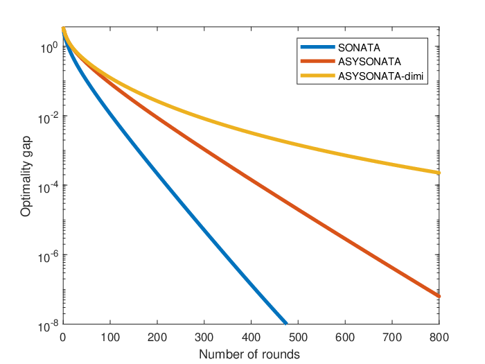
Figure 1: Directed graphs: optimality gap JkJ^{k} versus number of rounds.

We test ASY-SONATA with a constant step size γ=3.5\gamma=3.5, and also a diminishing step-size rule with each agent updating its local step size according to αt+1=αt​(1−0.001⋅αt)\alpha^{t+1}=\alpha^{t}\left(1-0.001\cdot\alpha^{t}\right) and α0=3.5\alpha^{0}=3.5; as benchmark, we also simulate its synchronous instance, with step size γ=0.8\gamma=0.8. In Fig. 1, we plot Jk≜(1/I)​∑i=1I‖𝐱ik−𝐱⋆‖22J^{k}\triangleq({1}/{I})\,\sqrt{\sum_{i=1}^{I}\|\mathbf{x}_{i}^{k}-\mathbf{x}^{\star}\|_{2}^{2}} versus the number of rounds (one round corresponds to one update of all the agents). The curves are averaged over 100100 Monte-Carlo simulations, with different graph and data instantiations. The plot clearly shows linear convergence of ASY-SONATAwith a constant step-size.

V-B Binary classification

In this subsection, we consider a strongly convex and nonconvex instance of Problem (P) over digraphs, namely: the regularized logistic regression (RLR) and the robust classification (RC) problems. Both formulations can be abstracted as:

min𝐱⁡1|𝒟|​∑i=1I∑j∈𝒟iV⁡(yj⋅ℓ𝐱​(𝐮j))+λ​‖∇ℓ𝐱​(⋅)‖22,\min_{\mathbf{x}}\frac{1}{\left|\mathcal{D}\right|}\sum_{i=1}^{I}\sum_{j\in\mathcal{D}_{i}}V(y_{j}\cdot\ell_{\mathbf{x}}(\mathbf{u}_{j}))+\lambda\left\lVert\nabla\ell_{\mathbf{x}}(\cdot)\right\rVert_{2}^{2},\vskip-2.84544pt (16)

where 𝒟=∪i=1I𝒟i\mathcal{D}=\cup_{i=1}^{I}\mathcal{D}_{i} is the set of indices of the data distributed across the agents, with agent ii owning 𝒟i\mathcal{D}_{i}, and 𝒟i∩𝒟l=∅,\mathcal{D}_{i}\cap\mathcal{D}_{l}=\emptyset, for all i≠li\neq l; 𝐮j\mathbf{u}_{j} and yj∈{−1,1}y_{j}\in\{-1,1\} are the feature vector and associated label of the jj-th sample in 𝒟\mathcal{D}; ℓ𝐱​(⋅)\ell_{\mathbf{x}}(\cdot) is a linear function, parameterized by 𝐱\mathbf{x}; and VV is the loss function. More specifically, if the RLR problem is considered, VV reads V⁡(r)=11+e−rV(r)=\frac{1}{1+e^{-r}} while for the RC problem, we have [42]

V⁡(r)={0,if ​r>1;14​r3−34​r+12,if −1≤r≤1;1,if ​r<−1.\displaystyle V(r)=\begin{cases}0,&\text{if }r>1;\\ \frac{1}{4}r^{3}-\frac{3}{4}r+\frac{1}{2},&\text{if }-1\leq r\leq 1;\\ 1,&\text{if }r<-1.\end{cases}

Data: We use the following data sets for the RLR and RC problems. (RLR): We set ℓ𝐱​(𝐮)=𝐱⊤​𝐮\ell_{\mathbf{x}}(\mathbf{u})=\mathbf{x}^{\top}\mathbf{u}, n=100n={100}, each |𝒟i|=20,\left|\mathcal{D}_{i}\right|=20, and λ=0.01.\lambda=0.01. The underlying statistical model is the following: We generated the ground truth 𝐱^\widehat{\mathbf{x}} with i.i.d. 𝒩⁡(0,1)\mathcal{N}(0,1) components; each training pair (𝐮j,yj)(\mathbf{u}_{j},y_{j}) is generated independently, with each element of 𝐮j\mathbf{u}_{j} being i.i.d. 𝒩⁡(0,1)\mathcal{N}(0,1) and yjy_{j} is set as 11 with probability V⁡(ℓ𝐱^​(𝐮j)),V(\ell_{\widehat{\mathbf{x}}}(\mathbf{u}_{j})), and −1-1 otherwise. (RC): We use the Cleveland Heart Disease Data set with 14 features [43], preprocessing it by deleting observations with missing entries, scaling features between 0-1, and distributing the data to agents evenly. We set ℓ𝐱​(𝐮)=𝐞15⊤​𝐱+∑d=114𝐞d⊤​𝐱​𝐞d⊤​𝐮.\ell_{\mathbf{x}}(\mathbf{u})=\mathbf{e}_{15}^{\top}\mathbf{x}+\sum_{d=1}^{14}\mathbf{e}_{d}^{\top}\mathbf{x}\,\mathbf{e}_{d}^{\top}\mathbf{u}. Network model: We simulated a digraph of I=30I=30 agents. Each agent has 77 out-neighbors; one of them belongs to a directed cycle connecting all the agents while the other 66 are picked uniformly at random. One row and one column stochastic matrix with uniform weights are generated. Asynchronous model: a) Activation lists are generated by concatenating random rounds. To generate one round, we first sample its length uniformly from the interval [I,T][I,T], with T=90.T=90. Within a round, we first have each agent appearing exactly once and then sample agents uniformly for the remaining spots. Finally a random shuffle of the agents order is performed on each round; b) Each transmitted message has (integer) traveling time which is sampled uniformly from the interval [0,Dtv][0,D^{\text{tv}}], with Dtv=90D^{\text{tv}}=90.

We compare the performance of our algorithm with AsySubPush [44] and AsySPA [45], which appeared online during the revision process of our paper. AsySubPush and AsySPA differ from ASY-SONATA in the following aspects: i) they do not employ any gradient tracking mechanism; ii) they cannot handle packet losses and purge out old information from the system (information is used as it is received); iii) when FF is strongly convex, they provably converge at sublinear rate; and iv) they cannot handle nonconvex FF. The step sizes of all algorithms are manually tuned to obtain the best practical performance. We run two instances of ASY-SONATA, one employing a constant step size γ=0.4\gamma=0.4 and the other one using the diminishing step size rule αt+1=αt​(1−0.001⋅αt)\alpha^{t+1}=\alpha^{t}\left(1-0.001\cdot\alpha^{t}\right), where α0=0.5\alpha^{0}=0.5 and tt is the local iteration counter. For AsySubPush (resp. AsySPA) we set, for each agent ii, αi=0.0001\alpha_{i}=0.0001 (resp. ρ⁡(k)=c/k\rho(k)={c}/{\sqrt{k}} with c=0.01c=0.01) in RLC and αi=0.00001\alpha_{i}=0.00001 (resp. ρ⁡(k)=c/k\rho(k)={c}/{\sqrt{k}} with c=0.001c=0.001) in RC. The result is averaged over 20 Monte Carlo experiments with different digraph instances, and is presented in Fig. 2; for each algorithm, we plot the merit functions MscM_{\text{sc}} (left panel) and MFM_{\text{F}} (right panel) evaluated in the generated trajectory versus the global iteration counter kk. Consistently with the convergence theory, ASY-SONATA with a constant step size exhibits a linear convergence rate. Also, ASY-SONATA outperforms the other two algorithms; this is mainly due to i) the presence in ASY-SONATA of an asynchronous gradient tracking mechanism which provides, at each iteration, a better estimate of ∇F\nabla F; and ii) the possibility in ASY-SONATA to discard old information when received after a newer one [cf. (5)].

Refer to caption
Figure 2: L: regularized logistic regression; R: robust classification.

VI Convergence Analysis of P-ASY-SUM-PUSH

We prove Theorem 7; we assume n=1n=1, without loss of generality. The proof is organized in the following two steps. Step 1: We first reduce the asynchronous agent system to a synchronous “augmented” one with no delays. This will be done adding virtual agents to the graph 𝒢\mathcal{G} along with their state variables, so that P-ASY-SUM-PUSH will be rewritten as a (synchronous) perturbed push-sum algorithm on the augmented graph. While this idea was first explored in [30, 31], there are some important differences between the proposed enlarged systems and those used therein, see Remark 13. Step 2: We conclude the proof establishing convergence of the perturbed push-sum algorithm built in Step 1.

VI-A Step 1: Reduction to a synchronous perturbed push-sum

VI-A1 The augmented graph

We begin constructing the augmented graph–an enlarged agent system obtained adding virtual agents to the original graph 𝒢=(𝒱,ℰ)\mathcal{G}=(\mathcal{V},\mathcal{E}). Specifically, we associate to each edge (j,i)∈ℰ(j,i)\in\mathcal{E} an ordered set of virtual nodes (agents), one for each of the possible delay values, denoted with a slight abuse of notation by (j,i)0,(j,i)1,…,(j,i)D(j,i)^{0},(j,i)^{1},\ldots,(j,i)^{D}; see Fig. 3. Roughly speaking, these virtual nodes store the “information on fly” based upon its associated delay, that is, the information that has been generated by j∈𝒩iinj\in\mathcal{N}^{\text{in}}_{i} for ii but not used (received) by ii yet. Adopting the terminology in [31], nodes in the original graph 𝒢\mathcal{G} are termed computing agents while the virtual nodes will be called noncomputing agents. With a slight abuse of notation, we define the set of computing and noncomputing agents as 𝒱^≜𝒱∪{(i,j)d|(i,j)∈ℰ,d=0,1,…,D}\widehat{\mathcal{V}}\triangleq\mathcal{V}\cup\{(i,j)^{d}\lvert\,(i,j)\in\mathcal{E},\,d=0,1,\ldots,D\}, and its cardinality as S≜|𝒱^|=(I+(D+1)​|ℰ|)S\triangleq\left|\widehat{\mathcal{V}}\right|=\left(I+(D+1)\left|\mathcal{E}\right|\right). We now identify the neighbors of each agent in this augmented systems. Computing agents no longer communicate among themselves; each j∈𝒱j\in\mathcal{V} can only send information to the noncomputing nodes (j,i)0(j,i)^{0}, with i∈𝒩jouti\in\mathcal{N}^{\text{out}}_{j}. Each noncomputing agent (j,i)d(j,i)^{d} can either send information to the next noncomputing agent, that is (j,i)d+1(j,i)^{d+1} (if any), or to the computing agent ii; see Fig. 3(b).

Refer to caption
Figure 3: Example of augmented graph, when the maximum delay D=2D=2; three noncomputing agents are added for each edge (j,i)∈ℰ(j,i)\in\mathcal{E}.

To describe the information stored by the agents in the augmented system at each iteration, let us first introduce the following quantities: 𝒯i≜{k|ik=i,k∈ℕ0}\mathcal{T}_{i}\triangleq\left\{k\,\big|\,i^{k}=i,\,k\in\mathbb{N}_{0}\right\} is the set of global iteration indices at which the computing agent i∈𝒱i\in\mathcal{V} wakes up; and, given k∈ℕ0k\in\mathbb{N}_{0}, let 𝒯ik≜{t∈𝒯i|t≤k}\mathcal{T}_{i}^{k}\triangleq\left\{t\in\mathcal{T}_{i}\,\big|\,t\leq k\right\}. It is not difficult to conclude from (7) and (8) that

ρi​jk=∑t∈𝒯jk−1ai​j​zjt+1/2​and​ρ~i​jk=ρi​jτi​jk−1,(j,i)∈ℰ.\hskip-14.22636pt\rho_{ij}^{k}=\!\sum_{t\in\mathcal{T}^{k-1}_{j}}a_{ij}z^{t+1/2}_{j}\,\,\,\text{and}\,\,\,\tilde{\rho}^{k}_{ij}=\!\rho_{ij}^{\tau_{ij}^{k-1}},\quad(j,i)\in\mathcal{E}.\vskip-8.5359pt (17)

At iteration k=0k=0, every computing agent ii stores zi0z_{i}^{0}, whereas the values of the noncomputing agents are initialized to 0.0. At the beginning of iteration kk, every computing agent ii will store zikz_{i}^{k} whereas every noncomputing agent (j,i)d(j,i)^{d}, with 0≤d≤D−10\leq d\leq D-1, stores the mass ai​j​zja_{ij}z_{j} (if any) generated by jj for ii at iteration k−d−1k-d-1 (thus k−d−1∈𝒯jk−1k-d-1\in\mathcal{T}_{j}^{k-1}), i.e., ai​j​zjk−(d+1)+1/2a_{ij}z_{j}^{k-(d+1)+1/2} (cf. Step 3.2), and not been used by ii yet (thus k−d>τi​jk−1k-d>\tau_{ij}^{k-1}); otherwise it stores 00. Formally, we have

z(j,i)dk≜\displaystyle\hskip-5.69046ptz^{k}_{(j,i)^{d}}\triangleq ai​j​zjt+1/2\displaystyle a_{ij}z_{j}^{t+1/2}
⋅𝟙[t=k−d−1∈𝒯jk−1&t+1>τi​jk−1].\displaystyle\cdot\mathbbm{1}{\left[t=k-d-1\in\mathcal{T}_{j}^{k-1}\,\,\&\,\,t+1>\tau_{ij}^{k-1}\right].} (18)

The virtual node (j,i)D(j,i)^{D} cumulates all the masses ai​j​zjk−(d+1)+1/2a_{ij}z_{j}^{k-(d+1)+1/2} with d≥Dd\geq D, not received by ii yet:

z(j,i)Dk≜∑t∈𝒯jk−D−1,t+1>τi​jk−1ai​j​zjt+1/2.\displaystyle z^{k}_{(j,i)^{D}}\triangleq\sum_{t\in\mathcal{T}_{j}^{k-D-1},\,t+1>\tau_{ij}^{k-1}}a_{ij}z_{j}^{t+1/2}. (19)

We write next P-ASY-SUM-PUSH on the augmented graph in terms of the zz-variables of both the computing and noncomputing agents, absorbing the (ρ,ρ~)(\rho,\tilde{\rho})-variables using (17)-(19).

The sum-step over the augmented graph. In the sum-step, the update of the zz-variables of the computing agents reads:

zikk+12=zikk+∑j∈𝒩ikin(ρik​jτik​jk−ρ~ik​jk)+ϵk\displaystyle z_{i^{k}}^{k+\frac{1}{2}}=z_{i^{k}}^{k}+\displaystyle\sum_{j\in\mathcal{N}_{i^{k}}^{\text{in}}}\left({\rho}^{\tau_{i^{k}j}^{k}}_{i^{k}j}-\tilde{\rho}_{i^{k}j}^{k}\right)+\epsilon^{k}\vskip-5.69046pt
=(17)−(19)​zikk+∑j∈𝒩ikin∑d=k−τik​jkDz(j,ik)dk+ϵk;\displaystyle\,\,\quad\overset{\eqref{eq:rho_z}-\eqref{eq:virtual_info}}{=}z_{i^{k}}^{k}+\displaystyle\sum_{j\in\mathcal{N}_{i^{k}}^{\text{in}}}\sum_{d=k-\tau_{i^{k}j}^{k}}^{D}z^{k}_{(j,i^{k})^{d}}+\epsilon^{k}; (20a)
zjk+12=zjk,j∈𝒱∖{ik}.z^{k+\frac{1}{2}}_{j}=z^{k}_{j},\quad j\in\mathcal{V}\setminus\{i^{k}\}.\vskip-5.69046pt (20b)
In words, node iki^{k} builds the update zikk→zikk+12z_{i^{k}}^{k}\!\!\to\!\!z_{i^{k}}^{k+\frac{1}{2}} based upon the masses transmitted by the noncomputing agents (j,ik)k−τik​jk,(j,ik)k−τik​jk+1,…,(j,i^{k})^{k-\tau_{i^{k}j}^{k}},(j,i^{k})^{k-\tau_{i^{k}j}^{k}+1},\ldots, (j,ik)D(j,i^{k})^{D} [cf. (20a)]. All the other computing agents keep their masses unchanged [cf. (20b)]. The updates of the noncomputing agents is set to
zk+12(j,ik)d≜0,d=k−τik​jk,…,D,j∈𝒩ikin;\displaystyle z^{k+\frac{1}{2}}_{(j,i^{k})^{d}}\triangleq 0,\quad d=k-\tau_{i^{k}j}^{k},\ldots,D,\quad j\in\mathcal{N}_{i^{k}}^{\text{in}};\vskip 3.0pt plus 1.0pt minus 1.0pt (20c)
z(j′,i)τk+12≜z(j′,i)τk,for all the other ​(j′,i)τ∈𝒱^.\displaystyle z^{k+\frac{1}{2}}_{(j^{\prime},i)^{\tau}}\triangleq z^{k}_{(j^{\prime},i)^{\tau}},\quad\text{for all the other }(j^{\prime},i)^{\tau}\in\widehat{\mathcal{V}}.\vskip-11.38092pt (20d)

The noncomputing agents in (20c) set their variables to zero (as they transferred their masses to iki^{k}) while the other noncomputing agents keep their variables unchanged [cf. (20d)]. Fig. 4 illustrates the sum-step over the augmented graph.

Refer to caption
Figure 4: Sum step on the augmented graph: τik​jk=k−1\tau_{i^{k}j}^{k}=k-1 (delay one); the two noncomputing agents, (j,ik)1(j,i^{k})^{1} and (j,ik)2(j,i^{k})^{2}, send their masses to ik.i^{k}.
Refer to caption
Figure 5: Push step on the augmented graph: Agent iki^{k} keeps aik​ik​zikk+1/2a_{i^{k}i^{k}}z_{i^{k}}^{k+1/2} while sending aℓ​ik​zikk+1/2a_{\ell i^{k}}z_{i^{k}}^{k+1/2} to the virtual nodes (ik,ℓ)0(i^{k},\ell)^{0}, ℓ∈𝒩ikout\ell\in\mathcal{N}_{i^{k}}^{\text{out}}.

The push-step over the augmented graph. In the push-step, the update of the zz-variables of the computing agents reads:

zikk+1=aik​ik​zikk+12;\displaystyle z_{i^{k}}^{k+1}=a_{i^{k}i^{k}}\,z_{i^{k}}^{k+\frac{1}{2}}; (21a)
zjk+1=zjk+12, for ​j∈𝒱∖{ik}.\displaystyle z^{k+1}_{j}=z^{k+\frac{1}{2}}_{j},\qquad\text{ for }j\in\mathcal{V}\setminus\{i^{k}\}. (21b)
In words, agent iki^{k} keeps the portion aik​ik​zikk+12a_{i^{k}i^{k}}{z}_{i^{k}}^{k+\frac{1}{2}} of the new generated mass [cf. (21a)] whereas the other computing agents do not change their variables [cf. (21b)]. The noncomputing agents update as:
z(ik,ℓ)0k+1≜aℓ​ik​zikk+1/2,ℓ∈𝒩ikout;\displaystyle z^{k+1}_{(i^{k},\ell)^{0}}\triangleq a_{\ell i^{k}}\,z_{i^{k}}^{k+1/2},\quad\ell\in\mathcal{N}_{i^{k}}^{\text{out}}; (21c)
z(i,j)0k+1≜0,(i,j)∈ℰ,i≠ik;\displaystyle z^{k+1}_{(i,j)^{0}}\triangleq 0,\quad(i,j)\in\mathcal{E},\quad i\neq i^{k}; (21d)
z(i,j)dk+1≜z(i,j)d−1k+12,d=1,…,D−1,(i,j)∈ℰ;\displaystyle z^{k+1}_{(i,j)^{d}}\triangleq z^{k+\frac{1}{2}}_{(i,j)^{d-1}},\quad d=1,\ldots,D-1,\quad(i,j)\in\mathcal{E}; (21e)
z(i,j)Dk+1≜z(i,j)Dk+12+z(i,j)D−1k+12,(i,j)∈ℰ.\displaystyle z^{k+1}_{(i,j)^{D}}\triangleq z^{k+\frac{1}{2}}_{(i,j)^{D}}+z^{k+\frac{1}{2}}_{(i,j)^{D-1}},\quad(i,j)\in\mathcal{E}. (21f)

In words, the computing agent iki^{k} pushes its masses aℓ​ik​zikk+12a_{\ell i^{k}}{z}_{i^{k}}^{k+\frac{1}{2}} to the noncomputing agents (ik,ℓ)0(i^{k},\ell)^{0}, with ℓ∈𝒩ikout\ell\in\mathcal{N}_{i^{k}}^{\text{out}} [cf. (21c)]. As the other noncomputing agents (i,j)0(i,j)^{0}, i≠iki\neq i^{k}, do not receive any mass for their associated computing agents, they set their variables to zero [cf. (21d)]. Finally the other noncomputing agents (i,j)d(i,j)^{d}, with 0≤d≤D−10\leq d\leq D-1, transfers their mass to the next noncomputing node (j,i)d+1(j,i)^{d+1} [cf. (21f), (21e)]. This push-step is illustrated in Fig. 5.

The following result establishes the equivalence between the update of the enlarged system with that of Algorithm 1.

Proposition 12.

Consider the setting of Theorem 7. The values of the zz-variables of the computing agents in (20)-(21) coincide with those of the zz-variables generated by P-ASY-SUM-PUSH (Algorithm 1), for all iterations k∈ℕ0k\in\mathbb{N}_{0}.

Proof.

By construction, the updates of the computing agents as in (20a)-(20b) and (21a)-(21b) coincide with the z-updates in the sum- and push-steps of P-ASY-SUM-PUSH, respectively. Therefore, we only need to show that the updates of the noncomputing agents are consistent with those of the (ρ,ρ~)(\rho,\tilde{\rho})-variables in P-ASY-SUM-PUSH. This follows using (17) and noting that the updates (21c)-(21f) are compliant with (18) and (19). For instance, by (17)-(18), it must be z(ik,j)0k+1=aj​ikzjt+1/2⋅𝟙[t=k∈𝒯ikk and t+1>τj​ikk]=aj​ikzjk+1/2z^{k+1}_{(i^{k},j)^{0}}=a_{ji^{k}}z_{j}^{t+1/2}\cdot\mathbbm{1}[t=k\in\mathcal{T}_{i^{k}}^{k}\text{ and }t+1>\tau_{ji^{k}}^{k}]=a_{ji^{k}}z_{j}^{k+1/2}, which in fact coincides with (21c). The other equations (21d)–(21f) can be similarly validated. ∎

Proposition 12 opens the way to study convergence of P-ASY-SUM-PUSH via that of the synchronous perturbed push-sum algorithm (20)-(21). To do so, it is convenient to rewrite (20)-(21) in vector-matrix form, as described next.

We begin introducing an enumeration rule for the components of the z-vector in the augmented system. We enumerate all the elements of ℰ\mathcal{E} as 1,2,…,|ℰ|.1,2,\ldots,\left|\mathcal{E}\right|. The computing agents in 𝒱^\widehat{\mathcal{V}} are indexed as in 𝒱\mathcal{V}, that is, 1,2,…,I1,2,\ldots,I. Each noncomputing agent (j,i)d(j,i)^{d} is indexed as I+d​|ℰ|+sI+d\left|\mathcal{E}\right|+s, where ss is the index associated with (j,i)(j,i) in ℰ\mathcal{E}; we will use interchangeably zI+d​|ℰ|+sz_{I+d\left|\mathcal{E}\right|+s} and z(j,i)d.z_{(j,i)^{d}}. We define the zz-vector as 𝐳^=[zi]i=1S\widehat{\mathbf{z}}=[{z}_{i}]_{i=1}^{S}; and its value at iteration k∈ℕ0k\in\mathbb{N}_{0} is denoted by 𝐳^k\widehat{\mathbf{z}}^{k}.

The transition matrix 𝐒k\mathbf{S}^{k} of the sum step is defined as

Sh​mk≜{1,if ​m∈{(j,ik)d∣k−τik​jk≤d≤D}and ​h=ik;1,if ​m∈𝒱^∖{(j,ik)d∣k−τik​jk≤d≤D}and ​h=m;0,otherwise.S_{hm}^{k}\triangleq\left\{\begin{aligned} &1,&&\text{if }m\in\{(j,i^{k})^{d}\mid k-\tau_{i^{k}j}^{k}\leq d\leq D\}\\ &&&\text{and }h=i^{k};\\ &1,&&\text{if }m\in\widehat{\mathcal{V}}\setminus\{(j,i^{k})^{d}\mid k-\tau_{i^{k}j}^{k}\leq d\leq D\}\\ &&&\text{and }h=m;\\ &0,&&\text{otherwise}.\end{aligned}\right.

Let 𝜺k≜ϵk​𝐞ik\bm{\varepsilon}^{k}\triangleq\epsilon^{k}\mathbf{e}_{i^{k}} be the S−S-dimensional perturbation vector. The sum-step can be written in compact form as

𝐳^k+12=𝐒k​𝐳^k+𝜺k.\widehat{\mathbf{z}}^{k+\frac{1}{2}}=\mathbf{S}^{k}\widehat{\mathbf{z}}^{k}+\bm{\varepsilon}^{k}.\vskip-2.84544pt (22)

Define the transition matrix 𝐏k\mathbf{P}^{k} of the push step as

Ph​mk≜{aj​ik,if m=ik and h=(j,ik)0,j∈𝒩ikout;aik​ik,if ​m=h=ik;1,if ​m=h∈𝒱∖ik;1,if m=(i,j)d,h=(i,j)d+1,(i,j)∈ℰ, 0≤d≤D−1;1,if m=h=(i,j)D,(i,j)∈ℰ;0,otherwiseP_{hm}^{k}\triangleq\left\{\begin{aligned} &a_{ji^{k}},&&\text{if }m=i^{k}\text{ and }h=(j,i^{k})^{0},j\in\mathcal{N}_{i^{k}}^{\text{out}};\\ &a_{i^{k}i^{k}},&&\text{if }m=h=i^{k};\\ &1,&&\text{if }m=h\in\mathcal{V}\setminus i^{k};\\ &1,&&\text{if }m=(i,j)^{d},\,h=(i,j)^{d+1},\\ &&&(i,j)\in\mathcal{E},\,0\leq d\leq D-1;\\ &1,&&\text{if }m=h=(i,j)^{D},\,(i,j)\in\mathcal{E};\\ &0,&&\text{otherwise}\end{aligned}\right.

Then, the push-step can be written as

𝐳^k+1=𝐏k​𝐳^k+12.\displaystyle\widehat{\mathbf{z}}^{k+1}=\mathbf{P}^{k}\widehat{\mathbf{z}}^{k+\frac{1}{2}}. (23)

Combing (22) and (23), yields

𝐳^k+1=𝐀^k​𝐳^k+𝐩k,𝐀^k≜𝐏k​𝐒k,𝐩k≜𝐏k​𝜺k.\displaystyle\widehat{\mathbf{z}}^{k+1}=\widehat{\mathbf{A}}^{k}\widehat{\mathbf{z}}^{k}+{\mathbf{p}}^{k},\quad\widehat{\mathbf{A}}^{k}\triangleq\mathbf{P}^{k}\mathbf{S}^{k},\quad{\mathbf{p}}^{k}\triangleq\mathbf{P}^{k}\bm{\varepsilon}^{k}. (24)

The updates of the ϕ\phi variables and the definition of the ϕ\phi-vector are similar as above. In summary, the P-ASY-SUM-PUSH algorithm can be rewritten in compact form as

𝐳^k+1=𝐀^k​𝐳^k+𝐩k,𝐩k=ϵk​𝐏k​𝐞ik;\displaystyle{\widehat{\mathbf{z}}}^{k+1}={\widehat{\mathbf{A}}}^{k}{\widehat{\mathbf{z}}}^{k}+{\mathbf{p}}^{k},\quad{\mathbf{p}}^{k}=\epsilon^{k}\,\mathbf{P}^{k}\,\mathbf{e}_{i^{k}}; (25a)
ϕ^k+1=𝐀^k​ϕ^k;\displaystyle{\widehat{\bm{\phi}}}^{k+1}={\widehat{\mathbf{A}}}^{k}{\widehat{\bm{\phi}}}^{k}; (25b)

with initialization: zi0∈ℝz^{0}_{i}\in\mathbb{R} and ϕi0=1\phi^{0}_{i}=1, for i∈𝒱i\in\mathcal{V}; and zi0=0z^{0}_{i}=0 and ϕi0=0\phi^{0}_{i}=0, for i∈𝒱^∖𝒱i\in\widehat{\mathcal{V}}\setminus\mathcal{V}.

Remark 13 (Comparison with [30, 31, 32, 38]).

The idea of reducing asynchronous (consensus) algorithms into synchronous ones over an augmented system was already explored in [31, 32, 38]. However, there are several important differences between the models therein and the proposed augmented graph. First of all, [38] extends the analysis in [30] to deal with asynchronous activations, but both work consider only packet losses (no delays). Second, our augmented graph model departs from that in [31, 32] in the following aspects: i) in our model, the virtual nodes are associated with the edges of the original graph rather than the nodes; ii) the noncomputing nodes store the information on fly (i.e., generated by a sender but not received by the intended receiver yet), while in [31, 32], each noncomputing agent owns a delayed copy of the message generated by the associated computing agent; and iii) the dynamics (25) over the augmented graph used to describe the P-ASY-SUM-PUSH procedure is different from those of the asynchronous consensus schemes [31, (1)] and [32, (1)].

VI-B Step 2: Proof of Theorem 7

VI-B1 Preliminaries

We begin studying some properties of the matrix product 𝐀^k:t\widehat{\mathbf{A}}^{k:t}, which will be instrumental to prove convergence of the perturbed push-sum scheme (25).

Lemma 14.

Let {𝐀^k}k∈ℕ0\{\widehat{\mathbf{A}}^{k}\}_{k\in\mathbb{N}_{0}} be the sequence of matrices in (25), generated by Algorithm 1, under Assumption 6, and with 𝐀≜(ai​j)i,j=1I\mathbf{A}\triangleq(a_{ij})_{i,j=1}^{I} satisfying Assumption 4 (i),(iii). The following hold: for all k∈ℕ0k\in\mathbb{N}_{0}, a) 𝐀^k\widehat{\mathbf{A}}^{k} is column stochastic; and b) the entries of the first II rows of 𝐀^k+K1−1:k\widehat{\mathbf{A}}^{k+K_{1}-1:k} are uniformly lower bounded by η≜m¯K1∈(0,1)\eta\triangleq\bar{m}^{K_{1}}\in(0,1), with K1≜(2​I−1)⋅T+I⋅DK_{1}\triangleq(2I-1)\cdot T+I\cdot D.

Proof.

The lemma essentially proves that (𝐀^k+K1−1:k)⊤(\widehat{\mathbf{A}}^{k+K_{1}-1:k})^{\top} is a SIA (Stochastic Indecomposable Aperiodic) matrix [32], by showing that for any time length of K1K_{1} iterations, there exists a path from any node mm in the augmented graph to any computing node h.h. While at a high level the proof shares some similarities with that of [31, Lemma 2] and [32, Lemma 5 (a)], there are important differences due to the distinct modeling of our augmented system. The complete proof is in Appendix -A. ∎

The key result of this section is stated next and shows that as k−tk-t increases, 𝐀^k:t\widehat{\mathbf{A}}^{k:t} approaches a column stochastic rank one matrix at a linear rate. Given Lemma 14, the proof follows the path of [31, Lemma 4, Lemma 5], [32, Lemma 4, Lemma 5(b,c)] and thus is omitted.

Lemma 15.

In the setting above, there exists a sequence of stochastic vectors {𝛏k}k∈ℕ0\{{\bm{\xi}}^{k}\}_{k\in\mathbb{N}_{0}} such that, for any k≥t∈ℕ0k\geq t\in\mathbb{N}_{0} and i,j∈{1,⋯,S}i,\,j\in\{1,\cdots,S\}, there holds

|A^k:ti​j−ξki|≤Cρk−t,\left|{\widehat{A}}^{k:t}_{ij}-\xi^{k}_{i}\right|\leq C\rho^{k-t},\vskip-5.69046pt (26)

with

C≜2​1+m¯−K11−m¯K1,ρ≜(1−m¯K1)1K1∈(0,1).C\triangleq 2\frac{1+\bar{m}^{-K_{1}}}{1-\bar{m}^{K_{1}}},\quad\rho\triangleq(1-\bar{m}^{K_{1}})^{\frac{1}{K_{1}}}\in(0,1).

Furthermore, ξik≥η\xi_{i}^{k}\geq\eta, for all i∈𝒱i\in\mathcal{V} and k∈ℕ0k\in\mathbb{N}_{0}.

VI-B2 Proof of Theorem 7

Applying (25) telescopically, yields: 𝐳^k+1=𝐀^k:0𝐳^0+∑l=1k𝐀^k:l𝐩l−1+𝐩k{\widehat{\mathbf{z}}}^{k+1}={\widehat{\mathbf{A}}}^{k:0}{\widehat{\mathbf{z}}}^{0}+\sum_{l=1}^{k}{\widehat{\mathbf{A}}}^{k:l}{\mathbf{p}}^{l-1}+{\mathbf{p}}^{k} and ϕ^k+1=𝐀^k:0ϕ^0,{\widehat{\bm{\phi}}}^{k+1}={\widehat{\mathbf{A}}}^{k:0}{\widehat{\bm{\phi}}}^{0},which using the column stochasticity of 𝐀^k:t\widehat{\mathbf{A}}^{k:t}, yields

𝟏⊤​𝐳^k+1=𝟏⊤​𝐳^0+∑l=0k𝟏⊤​𝐩l,𝟏⊤​ϕ^k+1=𝟏⊤​ϕ^0=I.\displaystyle\hskip-11.38092pt\mathbf{1}^{\top}{\widehat{\mathbf{z}}}^{k+1}=\mathbf{1}^{\top}{\widehat{\mathbf{z}}}^{0}+\sum_{l=0}^{k}\mathbf{1}^{\top}{\mathbf{p}}^{l},\quad\mathbf{1}^{\top}{\widehat{\bm{\phi}}}^{k+1}=\mathbf{1}^{\top}{\widehat{\bm{\phi}}}^{0}=I. (27)

Using (27) and ϕik+1≥I​η\phi_{i}^{k+1}\geq I\eta, for all i∈𝒱i\in\mathcal{V} and k≥K1−1k\geq K_{1}-1 [due to Lemma 14(b)], we have: for i∈𝒱i\in\mathcal{V} and k≥K1−1k\geq K_{1}-1,

|zik+1ϕik+1−𝟏⊤​𝐳^k+1I|≤1I​η​|zik+1−ϕik+1I​(𝟏⊤​𝐳^k+1)|\displaystyle\left|\frac{z_{i}^{k+1}}{\phi_{i}^{k+1}}-\frac{\mathbf{1}^{\top}{\widehat{\mathbf{z}}}^{k+1}}{I}\right|\leq\frac{1}{I\eta}\left|z_{i}^{k+1}-\frac{\phi_{i}^{k+1}}{I}(\mathbf{1}^{\top}{\widehat{\mathbf{z}}}^{k+1})\right|
≤1I​η​|zik+1−ξik​𝟏⊤​𝐳^k+1|+1I​η​|(ξik−ϕik+1I)​𝟏⊤​𝐳^k+1|\displaystyle\leq\frac{1}{I\eta}\left|z_{i}^{k+1}-\xi_{i}^{k}\mathbf{1}^{\top}{\widehat{\mathbf{z}}}^{k+1}\right|+\frac{1}{I\eta}\left|\left(\xi_{i}^{k}-\frac{\phi_{i}^{k+1}}{I}\right)\mathbf{1}^{\top}{\widehat{\mathbf{z}}}^{k+1}\right|
≤1I​η​|zik+1−ξik​𝟏⊤​𝐳^k+1|\displaystyle\leq\frac{1}{I\eta}\left|z_{i}^{k+1}-\xi_{i}^{k}\mathbf{1}^{\top}{\widehat{\mathbf{z}}}^{k+1}\right|
+1I​η|ξik−𝐀^i,:k:0ϕ^0I|⋅|𝟏⊤𝐳^0+∑l=0k𝟏⊤𝐩l|\displaystyle\quad+\frac{1}{I\eta}\left|\xi_{i}^{k}-\frac{{\widehat{\mathbf{A}}}_{i,:}^{k:0}{\widehat{\bm{\phi}}}^{0}}{I}\right|\cdot\left|\mathbf{1}^{\top}{\widehat{\mathbf{z}}}^{0}+\sum_{l=0}^{k}\mathbf{1}^{\top}{\mathbf{p}}^{l}\right|
≤(26)​1I​η​|zik+1−ξik​𝟏⊤​𝐳^k+1|+C​ρkI​η​(‖𝐳0‖+∑l=0k|ϵl|)\displaystyle\overset{\eqref{eq:Lemma_exp_decay}}{\leq}\frac{1}{I\eta}\left|z_{i}^{k+1}-\xi_{i}^{k}\mathbf{1}^{\top}{\widehat{\mathbf{z}}}^{k+1}\right|+\frac{C\rho^{k}}{\sqrt{I}\eta}\left(\left\lVert{\mathbf{z}}^{0}\right\rVert+\sum_{l=0}^{k}\left|\epsilon^{l}\right|\right) (28)

The next lemma provides a bound of |zik+1−ξik​𝟏⊤​𝐳^k+1|.\left|z_{i}^{k+1}-\xi_{i}^{k}\mathbf{1}^{\top}{\widehat{\mathbf{z}}}^{k+1}\right|.

Lemma 16.

Let {𝐳^k}k=0∞\{\widehat{\mathbf{z}}^{k}\}_{k=0}^{\infty} be the sequence generated by the perturbed system (25a), under Assumption 6, 𝐀=(ai​j)i,j=1I\mathbf{A}=(a_{ij})_{i,j=1}^{I} satisfying Assumption 4 (i), (iii), and given {ϵk}k∈ℕ0\{\epsilon^{k}\}_{k\in\mathbb{N}_{0}}. For any i∈𝒱i\in\mathcal{V} and k≥0k\geq 0, there holds

|zik+1−ξik​𝟏⊤​𝐳^k+1|≤C0​(ρk​‖𝐳0‖+∑l=0kρk−l​|ϵl|),\displaystyle\left|z_{i}^{k+1}-\xi_{i}^{k}\mathbf{1}^{\top}{\widehat{\mathbf{z}}}^{k+1}\right|\leq C_{0}\left(\rho^{k}\left\lVert\mathbf{z}^{0}\right\rVert+\sum_{l=0}^{k}\rho^{k-l}\left|\epsilon^{l}\right|\right), (29)

with {𝛏k}n∈ℕ0\{{\bm{\xi}}^{k}\}_{n\in\mathbb{N}_{0}} defined in Lemma 15 and C0≜C​2​S/ρ.C_{0}\triangleq C\sqrt{2S}/\rho.

Proof.
|zik+1−ξik𝟏⊤𝐳^k+1|=(25a)|(𝐀^i,:k:0𝐳^0+∑l=1k𝐀^i,:k:l𝐩l−1+pik)\displaystyle\left|z_{i}^{k+1}-\xi_{i}^{k}\mathbf{1}^{\top}{\widehat{\mathbf{z}}}^{k+1}\right|\overset{\eqref{eq:ordy_1}}{=}\Bigg|\left({\widehat{\mathbf{A}}}_{i,:}^{k:0}{\widehat{\mathbf{z}}}^{0}+\sum_{l=1}^{k}{\widehat{\mathbf{A}}}_{i,:}^{k:l}{\mathbf{p}}^{l-1}+{p}_{i}^{k}\right)
−ξik​(𝟏⊤​𝐳^0+∑l=0k𝟏⊤​𝐩l)|≤|pik|+|𝟏⊤​𝐩k|\displaystyle-\xi_{i}^{k}\left(\mathbf{1}^{\top}{\widehat{\mathbf{z}}}^{0}+\sum_{l=0}^{k}\mathbf{1}^{\top}{\mathbf{p}}^{l}\right)\Bigg|\leq\left|{p}_{i}^{k}\right|+\left|\mathbf{1}^{\top}{\mathbf{p}}^{k}\right|
+‖𝐀^i,:k:0−ξik𝟏⊤‖‖𝐳^0‖+∑l=1k‖𝐀^i,:k:l−ξik𝟏⊤‖‖𝐩l−1‖\displaystyle+\left\lVert{\widehat{\mathbf{A}}}_{i,:}^{k:0}-\xi_{i}^{k}\mathbf{1}^{\top}\right\rVert\left\lVert{\widehat{\mathbf{z}}}^{0}\right\rVert+\sum_{l=1}^{k}\left\lVert{\widehat{\mathbf{A}}}_{i,:}^{k:l}-\xi_{i}^{k}\mathbf{1}^{\top}\right\rVert\left\lVert{\mathbf{p}}^{l-1}\right\rVert
≤(26)​Sρ​C​(ρk​‖𝐳^0‖+∑l=0kρk−l​‖𝐏l‖​|ϵl|)\displaystyle\overset{\eqref{eq:Lemma_exp_decay}}{\leq}\frac{\sqrt{S}}{\rho}C\left(\rho^{k}\left\lVert{\widehat{\mathbf{z}}}^{0}\right\rVert+\sum_{l=0}^{k}\rho^{k-l}\left\lVert\mathbf{P}^{l}\right\rVert\left|\epsilon^{l}\right|\right)
≤(a)​C0​(ρk​‖𝐳0‖+∑l=0kρk−l​|ϵl|),\displaystyle\overset{(a)}{\leq}C_{0}\left(\rho^{k}\left\lVert\mathbf{z}^{0}\right\rVert+\sum_{l=0}^{k}\rho^{k-l}\left|\epsilon^{l}\right|\right),

where in (a) we used ‖𝐏l‖≤‖𝐏l‖1​‖𝐏l‖∞≤2.\left\lVert\mathbf{P}^{l}\right\rVert\leq\sqrt{\left\lVert\mathbf{P}^{l}\right\rVert_{1}\left\lVert\mathbf{P}^{l}\right\rVert_{\infty}}\leq\sqrt{2}. ∎

Combing Eq. (28) and (29) leads to

|zik+1ϕik+1−𝟏⊤​𝐳^k+1I|≤C1​(ρk​‖𝐳0‖+∑l=0kρk−l​|ϵl|),\displaystyle\left|\frac{z_{i}^{k+1}}{\phi_{i}^{k+1}}-\frac{\mathbf{1}^{\top}{\widehat{\mathbf{z}}}^{k+1}}{I}\right|\leq C_{1}\left(\rho^{k}\left\lVert\mathbf{z}^{0}\right\rVert+\sum_{l=0}^{k}\rho^{k-l}\left|\epsilon^{l}\right|\right),

where we defined C1≜C0⋅2/(I​η).C_{1}\triangleq C_{0}\cdot 2/(I\,\eta).

Recalling the definition of 𝔪zk≜∑i=1Izik+∑(j,i)∈ℰ(ρi​jk−ρ~i​jk)\mathfrak{m}^{k}_{z}\triangleq\sum_{i=1}^{I}{z}_{i}^{k}+\sum_{(j,i)\in\mathcal{E}}(\rho_{ij}^{k}-\tilde{\rho}_{ij}^{k}), to complete the proof, it remains to show that

𝔪zk​=(I)​∑i=1Izi0+∑t=0k−1ϵt​=(I​I)​𝟏⊤​𝐳^k.\mathfrak{m}^{k}_{z}\overset{(I)}{=}\sum_{i=1}^{I}{{z}_{i}^{0}}+\sum_{t=0}^{k-1}\epsilon^{t}\overset{(II)}{=}\mathbf{1}^{\top}\widehat{\mathbf{z}}^{k}. (30)

We prove next the equalities (I) and (II) separately.

Proof of (I): Since 𝔪z0=∑i=1Izi0\mathfrak{m}^{0}_{z}=\sum_{i=1}^{I}{{z}_{i}^{0}}, it suffices to show that 𝔪zk+1=𝔪zk+ϵk\mathfrak{m}^{k+1}_{z}=\mathfrak{m}^{k}_{z}+\epsilon^{k} for all k∈ℕ0k\in\mathbb{N}_{0}. Since agent iki^{k} triggers k→k+1,k\to k+1, we only need to show that

zikk+1+∑j∈𝒩ikin(ρik​jk+1−ρ~ik​jk+1)+∑j∈𝒩ikout(ρj​ikk+1−ρ~j​ikk+1)\displaystyle z_{i^{k}}^{k+1}+\sum_{j\in\mathcal{N}_{i^{k}}^{\text{in}}}({\rho}_{{i^{k}}j}^{k+1}-\tilde{{\rho}}_{{i^{k}}j}^{k+1})+\sum_{j\in\mathcal{N}_{{i^{k}}}^{\text{out}}}(\rho_{j{i^{k}}}^{k+1}-\tilde{\rho}_{j{i^{k}}}^{k+1})
=\displaystyle= zikk+∑j∈𝒩ikin(ρik​jk−ρ~ik​jk)+∑j∈𝒩ikout(ρj​ikk−ρ~j​ikk)+ϵk.\displaystyle z_{{i^{k}}}^{k}+\sum_{j\in\mathcal{N}_{{i^{k}}}^{\text{in}}}(\rho_{{i^{k}}j}^{k}-\tilde{\rho}_{{i^{k}}j}^{k})+\sum_{j\in\mathcal{N}_{i^{k}}^{\text{out}}}(\rho_{j{i^{k}}}^{k}-\tilde{\rho}_{j{i^{k}}}^{k})+\epsilon^{k}.

We have

zikk+1+∑j∈𝒩ikin(ρik​jk+1−ρ~ik​jk+1)+∑j∈𝒩ikout(ρj​ikk+1−ρ~j​ikk+1)\displaystyle z_{i^{k}}^{k+1}+\sum_{j\in\mathcal{N}_{i^{k}}^{\text{in}}}(\rho_{i^{k}j}^{k+1}-\tilde{\rho}_{i^{k}j}^{k+1})+\sum_{j\in\mathcal{N}_{i^{k}}^{\text{out}}}(\rho_{ji^{k}}^{k+1}-\tilde{\rho}_{ji^{k}}^{k+1})
=(a)\displaystyle\overset{(a)}{=} aik​ik​zikk+12+∑j∈𝒩ikin(ρik​jk−ρik​jτik​jk)\displaystyle a_{i^{k}i^{k}}z_{i^{k}}^{k+\frac{1}{2}}+\sum_{j\in\mathcal{N}_{i^{k}}^{\text{in}}}(\rho_{i^{k}j}^{k}-\rho_{i^{k}j}^{{\tau_{i^{k}j}^{k}}})
+∑j∈𝒩ikout(ρj​ikk+aj​ikzikk+12−ρ~j​ikk)\displaystyle+\sum_{j\in\mathcal{N}_{i^{k}}^{\text{out}}}(\rho_{ji^{k}}^{k}+a_{ji^{k}}z_{i^{k}}^{k+\frac{1}{2}}-\tilde{\rho}_{ji^{k}}^{k})
=(b)\displaystyle\overset{(b)}{=} zikk+12+∑j∈𝒩ikin(ρik​jk−ρik​jτik​jk)+∑j∈𝒩ikout(ρj​ikk−ρ~j​ikk)\displaystyle z_{i^{k}}^{k+\frac{1}{2}}+\sum_{j\in\mathcal{N}_{i^{k}}^{\text{in}}}(\rho_{i^{k}j}^{k}-\rho_{i^{k}j}^{{\tau_{i^{k}j}^{k}}})+\sum_{j\in\mathcal{N}_{i^{k}}^{\text{out}}}(\rho_{ji^{k}}^{k}-\tilde{\rho}_{ji^{k}}^{k})
=(c)\displaystyle\overset{(c)}{=} zikk+∑j∈𝒩ikin(ρik​jτik​jk−ρ~ik​jk)+ϵk+∑j∈𝒩ikin(ρik​jk−ρik​jτik​jk)\displaystyle z_{i^{k}}^{k}+\sum_{j\in\mathcal{N}_{i^{k}}^{{\text{in}}}}(\rho_{i^{k}j}^{{\tau_{i^{k}j}^{k}}}-\tilde{\rho}_{i^{k}j}^{k})+\epsilon^{k}+\sum_{j\in\mathcal{N}_{i^{k}}^{\text{in}}}(\rho_{i^{k}j}^{k}-\rho_{i^{k}j}^{{\tau_{i^{k}j}^{k}}})
+∑j∈𝒩ikout(ρj​ikk−ρ~j​ikk)\displaystyle+\sum_{j\in\mathcal{N}_{i^{k}}^{\text{out}}}(\rho_{ji^{k}}^{k}-\tilde{\rho}_{ji^{k}}^{k})
=\displaystyle= zikk+∑j∈𝒩ikin(ρik​jk−ρ~ik​jk)+∑j∈𝒩ikout(ρj​ikk−ρ~j​ikk)+ϵk,\displaystyle z_{i^{k}}^{k}+\sum_{j\in\mathcal{N}_{i^{k}}^{\text{in}}}(\rho_{i^{k}j}^{k}-\tilde{\rho}_{i^{k}j}^{k})+\sum_{j\in\mathcal{N}_{i^{k}}^{\text{out}}}(\rho_{ji^{k}}^{k}-\tilde{\rho}_{ji^{k}}^{k})+\epsilon^{k},

where in (a) we used: the definition of the push step, ρik​jk+1=ρik​jk\rho_{i^{k}j}^{k+1}=\rho_{i^{k}j}^{k} for all j∈𝒩ikinj\in\mathcal{N}_{i^{k}}^{\text{in}}, and ρ~j​ikk+1=ρ~j​ikk\tilde{\rho}_{ji^{k}}^{k+1}=\tilde{\rho}_{ji^{k}}^{k} for all j∈𝒩ikoutj\in\mathcal{N}_{i^{k}}^{\text{out}}; (b) follows from aik​ik+∑j∈𝒩ikoutaj​ik=1a_{i^{k}i^{k}}+\sum_{j\in\mathcal{N}_{i^{k}}^{\text{out}}}a_{ji^{k}}=1; and in (c), we used the sum-step.

Proof of (II): Using (27), yields 𝟏⊤​𝐳^k+1=𝟏⊤​𝐳^0+∑l=0k𝟏⊤​𝐩l=𝟏⊤​𝐳^k+𝟏⊤​𝜺k=∑i=1Izi0+∑t=0kϵt\mathbf{1}^{\top}\widehat{\mathbf{z}}^{k+1}=\mathbf{1}^{\top}{\widehat{\mathbf{z}}}^{0}+\sum_{l=0}^{k}\mathbf{1}^{\top}{\mathbf{p}}^{l}=\mathbf{1}^{\top}\widehat{\mathbf{z}}^{k}+\mathbf{1}^{\top}\bm{\varepsilon}^{k}=\sum_{i=1}^{I}{{z}_{i}^{0}}+\sum_{t=0}^{k}\epsilon^{t}.∎

VII ASY-SONATA–Proof of Theorem 9

We organize the proof in the following steps: Step 1: We introduce and study convergence of an auxiliary perturbed consensus scheme, which serves as a unified model for the descent and consensus updates in ASY-SONATA–the main result is summarized in Proposition 18; Step 2: We introduce the consensus and gradient tracking errors along with a suitably defined optimization error; and we derive bounds connecting these quantities, building on results in Step 1 and convergence of P-ASY-SUM-PUSH–see Proposition 19. The goal is to prove that the aforementioned errors vanish at a linear rate. To do so, Step 3 introduces a general form of the small gain theorem–Theorem 23–along with some technical results, which allows us to establish the desired linear convergence through the boundedness of the solution of an associated linear system of inequalities. Step 4 builds such a linear system for the error quantities introduced in Step 2 and proves the boundedness of its solution, proving thus Theorem 9. The rate expression (13) is derived in Appendix -D. Through the proof we assume n=1n=1 (scalar variables); and define CL≜maxi=1,…,I⁡LiC_{L}\triangleq\max_{i=1,\ldots,I}L_{i} and L≜∑i=1ILi.L\triangleq\sum_{i=1}^{I}L_{i}.

Step 1: A perturbed asynchronous consensus scheme

We introduce a unified model to study the dynamics of the consensus and optimization errors in ASY-SONATA, which consists in pulling out the tracking update (Step 5) and treat the z-variables–the term −γk​zikk-\gamma^{k}z_{i^{k}}^{k} in (11)–as an exogenous perturbation δk\delta^{k}. More specifically, consider the following scheme (with a slight abuse of notation, we use the same symbols as in ASY-SONATA):

vikk+1=xikk+δk,\displaystyle v_{i^{k}}^{k+1}=x_{i^{k}}^{k}+\delta^{k}, (31a)
xikk+1=wik​ik​vikk+1+∑j∈𝒩ikinwik​j​vjk−djk,\displaystyle x_{i^{k}}^{k+1}=w_{i^{k}i^{k}}v_{i^{k}}^{k+1}+\sum_{j\in\mathcal{N}_{i^{k}}^{\text{in}}}w_{{i^{k}}j}v_{j}^{k-d_{j}^{k}}, (31b)
vjk+1=vjk,xjk+1=xjk,∀j∈𝒱∖{ik},\displaystyle v_{j}^{k+1}=v_{j}^{k},\,x_{j}^{k+1}=x_{j}^{k},\quad\forall j\in\mathcal{V}\setminus\{i^{k}\}, (31c)

with given xi0∈ℝx_{i}^{0}\in\mathbb{R}, vit=0v_{i}^{t}=0, t=−D,−D+1,…,0t=-D,-D+1,\ldots,0, for all i∈𝒱~i\in\tilde{\mathcal{V}}. We make the blanket assumption that agents’ activations and delays satisfy Assumption 6.

Let us rewrite (31) in a vector-matrix form. Define 𝐱k≜[x1k,⋯,xIk]⊤\mathbf{x}^{k}\triangleq[{x}_{1}^{k},\cdots,{x}_{I}^{k}]^{\top} and 𝐯k≜[v1k,⋯,vIk]⊤\mathbf{v}^{k}\triangleq[{v}_{1}^{k},\cdots,{v}_{I}^{k}]^{\top}. Construct the (D+2)​I(D+2)I dimensional concatenated vectors

𝐡k≜[𝐱k⊤,𝐯k⊤,𝐯k−1⊤,⋯,𝐯k−D⊤]⊤,𝜹k≜δk​𝐞ik;\hskip-5.69046pt\mathbf{h}^{k}\triangleq[{\mathbf{x}^{k}}^{\top},{\mathbf{v}^{k}}^{\top},{\mathbf{v}^{k-1}}^{\top},\cdots,{\mathbf{v}^{k-D}}^{\top}]^{\top},\quad{\bm{\delta}}^{k}\triangleq\delta^{k}\,\mathbf{e}_{i^{k}}; (32)

and the augmented matrix 𝐖^k\widehat{\mathbf{W}}^{k}, defined as

W^r​mk≜{wik​ik,if ​r=m=ik;wik​j,if r=ik,m=j+(djk+1)I;1,if ​r=m∈{1,2,…,2​I}∖{ik,ik+I};1,if ​r∈{2​I+1,2​I+2,…,(D+2)​I}∪{ik+I}​ and ​m=r−I;0,otherwise.\widehat{W}_{rm}^{k}\triangleq\left\{\begin{aligned} &w_{i^{k}i^{k}},&&\text{if }r=m=i^{k};\\ &w_{i^{k}j},&&\text{if }r=i^{k},\,m=j+(d_{j}^{k}+1)I;\\ &1,&&\text{if }r=m\in\{1,2,\ldots,2I\}\setminus\{i^{k},i^{k}+I\};\\ &1,&&\text{if }r\in\{2I+1,2I+2,\ldots,(D+2)I\}\\ &&&\cup\{i^{k}+I\}\text{ and }m=r-I;\\ &0,&&\text{otherwise}.\end{aligned}\right.

System (31) can be rewritten in compact form as

𝐡k+1=𝐖^k​(𝐡k+𝜹k),\displaystyle\mathbf{\mathbf{h}}^{k+1}=\widehat{\mathbf{W}}^{k}(\mathbf{\mathbf{h}}^{k}+{\bm{\delta}}^{k}), (33)

The following lemma captures the asymptotic behavior of 𝐖^k\widehat{\mathbf{W}}^{k}.

Lemma 17.

Let {𝐖^k}k∈ℕ0\{\widehat{\mathbf{W}}^{k}\}_{k\in\mathbb{N}_{0}} be the sequence of matrices in (33), generated by (31), under Assumption 6 and with 𝐖\mathbf{W} satisfying Assumption 4 (i), (ii). The following hold: for all k∈ℕ0k\in\mathbb{N}_{0}, a) 𝐖^k\widehat{\mathbf{W}}^{k} is row stochastic; b) there exists a sequence of stochastic vectors {𝛙k}k∈ℕ0\{\bm{\psi}^{k}\}_{k\in\mathbb{N}_{0}} such that

‖𝐖^k:t−𝟏𝝍t⊤‖≤C2ρk−t,C2≜2​(D+2)​I​(1+m¯−K1)1−m¯−K1\hskip-5.69046pt\left\lVert\widehat{\mathbf{W}}^{k:t}-\mathbf{1}{\bm{\psi}^{t}}^{\top}\right\rVert\leq C_{2}\rho^{k-t},\quad C_{2}\triangleq\frac{2\sqrt{(D+2)I}(1+\bar{m}^{-K_{1}})}{1-\bar{m}^{-K_{1}}} (34)

Furthermore, ψik≥η=m¯K1\psi_{i}^{k}\geq\eta=\bar{m}^{K_{1}}, for all k≥0k\geq 0 and i∈𝒱i\in\mathcal{V}.

Proof.

The proof follows similar techniques as in [31, 32], and can be found in Appendix -G. ∎

We define now a proper consensus error for (33). Writing 𝐡k\mathbf{\mathbf{h}}^{k} in (33) recursively, yields

𝐡k+1=𝐖^k:0𝐡0+∑l=0k𝐖^k:l𝜹l.\mathbf{\mathbf{h}}^{k+1}=\widehat{\mathbf{W}}^{k:0}\mathbf{\mathbf{h}}^{0}+\sum_{l=0}^{k}\widehat{\mathbf{W}}^{k:l}{\bm{\delta}}^{l}.\vskip-2.84544pt (35)

Using Lemma 17, for any fixed N∈ℕ0N\in\mathbb{N}_{0}, we have

limk→∞(𝐖^k:0𝐡0+∑l=0N𝐖^k:l𝜹l)=𝟏𝝍0⊤𝐡0+∑l=0N𝟏𝝍l⊤𝜹l.\lim_{k\to\infty}(\widehat{\mathbf{W}}^{k:0}\mathbf{\mathbf{h}}^{0}+\sum_{l=0}^{N}\widehat{\mathbf{W}}^{k:l}{\bm{\delta}}^{l})=\mathbf{1}{\bm{\psi}^{0}}^{\top}\mathbf{\mathbf{h}}^{0}+\sum_{l=0}^{N}\mathbf{1}{\bm{\psi}^{l}}^{\top}{\bm{\delta}}^{l}.

Define

x𝝍0≜𝝍0⊤​𝐡0,x𝝍k+1≜𝝍0⊤​𝐡0+∑l=0k𝝍l⊤​𝜹l,k∈ℕ0.x_{\bm{\psi}}^{0}\triangleq{\bm{\psi}^{0}}^{\top}\mathbf{\mathbf{h}}^{0},\quad x_{\bm{\psi}}^{k+1}\triangleq{\bm{\psi}^{0}}^{\top}\mathbf{\mathbf{h}}^{0}+\sum_{l=0}^{k}{\bm{\psi}^{l}}^{\top}{\bm{\delta}}^{l},\,\,k\in\mathbb{N}_{0}.\vskip-5.69046pt (36)

Applying (36) inductively, it is easy to check that

x𝝍k+1=x𝝍k+𝝍k⊤​𝜹k=x𝝍k+ψikk​δk.x_{\bm{\psi}}^{k+1}=x_{\bm{\psi}}^{k}+{\bm{\psi}^{k}}^{\top}{\bm{\delta}}^{k}=x_{\bm{\psi}}^{k}+\psi_{i^{k}}^{k}\delta^{k}. (37)

We are now ready to state the main result of this subsection, which is a bound of the consensus disagreement ‖𝐡k+1−𝟏​x𝝍k+1‖\|\mathbf{h}^{k+1}-\mathbf{1}x_{\bm{\psi}}^{k+1}\| in terms of the magnitude of the perturbation.

Proposition 18.

In the above setting, the consensus error ‖𝐡k+1−𝟏​x𝛙k+1‖\|\mathbf{h}^{k+1}-\mathbf{1}x_{\bm{\psi}}^{k+1}\| satisfies: for all k∈ℕ0k\in\mathbb{N}_{0},

‖𝐡k+1−𝟏​x𝝍k+1‖≤C2​ρk​‖𝐡0−𝟏​x𝝍0‖+C2​∑l=0kρk−l​|δl|.\left\lVert\mathbf{h}^{k+1}-\mathbf{1}x_{\bm{\psi}}^{k+1}\right\rVert\leq C_{2}\rho^{k}\left\lVert\mathbf{\mathbf{h}}^{0}-\mathbf{1}x_{\bm{\psi}}^{0}\right\rVert+C_{2}\sum_{l=0}^{k}\rho^{k-l}\left|\delta^{l}\right|.\vskip-5.69046pt
Proof.

The proof follows readily from (35), (36), and Lemma 17; we omit further details.

∎

Step 2: Consensus, tracking, and optimization errors

1) Consensus disagreement: As anticipated, the updates of ASY-SONATA are also described by (31), if one sets therein δk=−γk​zikk\delta^{k}=-\gamma^{k}{z}_{i^{k}}^{k} (with zikk{z}_{i^{k}}^{k} satisfying Step 5 of ASY-SONATA). Let 𝐡k\mathbf{h}^{k} and x𝝍kx_{\bm{\psi}}^{k} be defined as in (32) and (36), respectively, with δk=−γk​zikk\delta^{k}=-\gamma^{k}{z}_{i^{k}}^{k}. The consensus error at iteration kk is defined as

E𝐜k≜‖𝐡k−𝟏​x𝝍k‖.E_{\mathbf{c}}^{k}\triangleq\left\lVert\mathbf{h}^{k}-\mathbf{1}x_{\bm{\psi}}^{k}\right\rVert.\vskip-2.84544pt (38)

2) Gradient tracking error: The gradient tracking step in ASY-SONATA is an instance of P-ASY-SUM-PUSH, with ϵk=∇fik​(𝐱ikk+1)−∇fik​(𝐱ikk)\epsilon^{k}=\nabla f_{i^{k}}(\mathbf{x}_{i^{k}}^{k+1})-\nabla f_{i^{k}}(\mathbf{x}_{i^{k}}^{k}). By Proposition 12, P-ASY-SUM-PUSH is equivalent to (25). In view of Lemma 16 and the following property 𝟏⊤​𝐳^k=∑i=1I∇fi​(xi0)+∑t=0k−1(∇fit​(xitt+1)−∇fit​(xitt))=∑i=1I∇fi​(xik)\mathbf{1}^{\top}\widehat{\mathbf{z}}^{k}=\sum_{i=1}^{I}\nabla f_{i}(x_{i}^{0})+\sum_{t=0}^{k-1}\left(\nabla f_{i^{t}}(x_{i^{t}}^{t+1})-\nabla f_{i^{t}}(x_{i^{t}}^{t})\right)=\sum_{i=1}^{I}\nabla f_{i}(x_{i}^{k}) where the first equality follows from (30) and ϵk=∇fik​(𝐱ikk+1)−∇fik​(𝐱ikk)\epsilon^{k}=\nabla f_{i^{k}}(\mathbf{x}_{i^{k}}^{k+1})-\nabla f_{i^{k}}(\mathbf{x}_{i^{k}}^{k}) while in the second equality we used xjt+1=xjtx_{j}^{t+1}=x_{j}^{t}, for j≠itj\neq i^{t}, the tracking error at iteration kk along with the magnitude of the tracking variables are defined as

E𝐭k≜|zikk−ξikk−1​g¯k|,E𝐳k≜|zikk|,g¯k≜∑i=1I∇fi​(xik),\hskip-5.69046ptE_{\mathbf{t}}^{k}\triangleq\left|{z}_{i^{k}}^{k}-\xi_{i^{k}}^{k-1}\,\bar{g}^{k}\right|,\,\,E_{\mathbf{z}}^{k}\triangleq\left|{z}_{i^{k}}^{k}\right|,\,\,\bar{g}^{k}\triangleq\sum_{i=1}^{I}\nabla f_{i}(x_{i}^{k}),\vskip-5.69046pt (39)

with ξi−1≜η\xi_{i}^{-1}\triangleq\eta, i∈𝒱i\in\mathcal{V}. Let 𝐠k≜[∇f1​(x1k),…,∇fI​(xIk)]⊤.\mathbf{g}^{k}\triangleq[\nabla f_{1}(x_{1}^{k}),\ldots,\nabla f_{I}(x_{I}^{k})]^{\top}.

3) Optimization error: Let x⋆x^{\star} be the unique minimizer of FF. Given the definition of consensus disagreement in (38), we define the optimization error at iteration kk as

E𝐨k≜|x𝝍k−x⋆|.E_{\mathbf{o}}^{k}\triangleq\left|x_{\bm{\psi}}^{k}-x^{\star}\right|. (40)

Note that this is a natural choice as, if consensual, all agents’ local variables will converge to a limit point of {x𝝍k}k∈ℕ0\{x_{\bm{\psi}}^{k}\}_{k\in\mathbb{N}_{0}}.

4) Connection among E𝐜kE_{\mathbf{c}}^{k}, E𝐭kE_{\mathbf{t}}^{k}, E𝐳kE_{\mathbf{z}}^{k}, and E𝐨kE_{\mathbf{o}}^{k}: The following proposition establishes bounds on the above quantities.

Proposition 19.

Let {𝐱k,𝐯k,𝐳k}k∈ℕ0\{\mathbf{x}^{k},\mathbf{v}^{k},\mathbf{z}^{k}\}_{k\in\mathbb{N}_{0}} be the sequence generated by ASY-SONATA, in the setting of Theorem 9, but possibly with a time-varying step-size {γk}k∈ℕ0\{\gamma^{k}\}_{k\in\mathbb{N}_{0}}. The error quantities E𝐜kE_{\mathbf{c}}^{k}, E𝐭kE_{\mathbf{t}}^{k}, E𝐳kE_{\mathbf{z}}^{k}, and E𝐨kE_{\mathbf{o}}^{k} satisfy: for all k∈ℕ0k\in\mathbb{N}_{0},

E𝐜k+1≤\displaystyle E_{\mathbf{c}}^{k+1}\leq C2​ρk​E𝐜0+C2​∑l=0kρk−l​γl​E𝐳l.\displaystyle C_{2}\rho^{k}E_{\mathbf{c}}^{0}+C_{2}\sum_{l=0}^{k}\rho^{k-l}\gamma^{l}E_{\mathbf{z}}^{l}. (41a)
E𝐭k+1≤\displaystyle E_{\mathbf{t}}^{k+1}\leq 3​C0​CL​∑l=0kρk−l​(E𝐜l+γl​E𝐳l)+C0​ρk​‖𝐠0‖;\displaystyle 3C_{0}C_{L}\sum_{l=0}^{k}\rho^{k-l}\left(E_{\mathbf{c}}^{l}+\gamma^{l}E_{\mathbf{z}}^{l}\right)+C_{0}\rho^{k}\left\lVert\mathbf{g}^{0}\right\rVert; (41b)
E𝐳k≤\displaystyle E_{\mathbf{z}}^{k}\,\,\leq E𝐭k+CL​I​E𝐜k+L​E𝐨k\displaystyle E_{\mathbf{t}}^{k}+C_{L}\sqrt{I}E_{\mathbf{c}}^{k}+L\,E_{\mathbf{o}}^{k} (41c)
Further assume γk≤1/L,k∈ℕ0;\gamma^{k}\leq 1/L,\,k\in\mathbb{N}_{0}; then
E𝐨k+1≤\displaystyle E_{\mathbf{o}}^{k+1}{\leq} ∑l=0k(∏t=l+1k(1−τ​η2​γt))​(CL​I​E𝐜l+E𝐭l)​γl\displaystyle\sum_{l=0}^{k}\bigg(\prod_{t=l+1}^{k}\left(1-\tau\eta^{2}\gamma^{t}\right)\bigg)\big(C_{L}\sqrt{I}E_{\mathbf{c}}^{l}+E_{\mathbf{t}}^{l}\big)\gamma^{l}
+∏t=0k(1−τη2γt)E𝐨0,\displaystyle+\prod_{t=0}^{k}\left(1-\tau\eta^{2}\gamma^{t}\right)E_{\mathbf{o}}^{0}, (41d)

where η∈(0,1)\eta\in(0,1) is defined in Lemma 15 and τ\tau is the strongly convexity constant of FF.

Proof.

Eq. (41a) follows readily from Proposition 18.

We prove now (41b). Recall 𝟏⊤​𝐳^k=g¯k\mathbf{1}^{\top}\widehat{\mathbf{z}}^{k}=\bar{g}^{k}. Using Lemma 16 with ϵk=∇fik​(𝐱ikk+1)−∇fik​(𝐱ikk)\epsilon^{k}=\nabla f_{i^{k}}(\mathbf{x}_{i^{k}}^{k+1})-\nabla f_{i^{k}}(\mathbf{x}_{i^{k}}^{k}), we obtain: for all i∈𝒱,i\in\mathcal{V},

|zik+1−ξik​g¯k+1|\displaystyle\left|{z}_{i}^{k+1}-\xi_{i}^{k}\,\bar{g}^{k+1}\right|
≤C0​(ρk​‖𝐠0‖+∑l=0kρk−l​|∇fill+1−∇fill|)\displaystyle\leq C_{0}\left(\rho^{k}\left\lVert\mathbf{g}^{0}\right\rVert+\sum_{l=0}^{k}\rho^{k-l}\left|\nabla f_{i^{l}}^{l+1}-\nabla f_{i^{l}}^{l}\right|\right)
≤C0​ρk​‖𝐠0‖+C0​CL​∑l=0kρk−l​|xill+1−xill|\displaystyle\leq C_{0}\,\rho^{k}\left\lVert\mathbf{g}^{0}\right\rVert+C_{0}C_{L}\sum_{l=0}^{k}\rho^{k-l}\left|{x}_{i^{l}}^{l+1}-{x}_{i^{l}}^{l}\right|
≤C0​ρk​‖𝐠0‖+C0​CL​∑l=0kρk−l​‖𝐡l+1−𝐡l‖\displaystyle\leq C_{0}\,\rho^{k}\left\lVert\mathbf{g}^{0}\right\rVert+C_{0}C_{L}\sum_{l=0}^{k}\rho^{k-l}\left\lVert\mathbf{h}^{l+1}-\mathbf{h}^{l}\right\rVert
=C0​ρk​‖𝐠0‖+C0​CL​∑l=0kρk−l​‖𝐖^l​(𝐡l+𝜹l)−𝐡l‖\displaystyle=C_{0}\rho^{k}\left\lVert\mathbf{g}^{0}\right\rVert+C_{0}C_{L}\sum_{l=0}^{k}\rho^{k-l}\left\lVert\widehat{\mathbf{W}}^{l}\left(\mathbf{\mathbf{h}}^{l}+{\bm{\delta}}^{l}\right)-\mathbf{h}^{l}\right\rVert
=(a)​C0​ρk​‖𝐠0‖\displaystyle\overset{(a)}{=}C_{0}\,\rho^{k}\left\lVert\mathbf{g}^{0}\right\rVert
+C0CL∑l=0kρk−l‖(𝐖^l−𝐈)(𝐡l−𝟏x𝝍l)−γlzill𝐖^l𝐞il‖\displaystyle+C_{0}C_{L}\sum_{l=0}^{k}\rho^{k-l}\left\lVert\big(\widehat{\mathbf{W}}^{l}-\mathbf{I}\big)\big(\mathbf{\mathbf{h}}^{l}-\mathbf{1}x_{\bm{\psi}}^{l}\big)-\gamma^{l}z_{i^{l}}^{l}\widehat{\mathbf{W}}^{l}\mathbf{e}_{i^{l}}\right\rVert
≤C0​ρk​‖𝐠0‖+C0​CL​∑l=0kρk−l​(‖𝐖^l‖​γl​E𝐳lCLOSE\displaystyle\leq C_{0}\rho^{k}\left\lVert\mathbf{g}^{0}\right\rVert+C_{0}C_{L}\sum_{l=0}^{k}\rho^{k-l}\Bigg(\|\widehat{\mathbf{W}}^{l}\|\gamma^{l}E_{\mathbf{z}}^{l}
OPEN+(‖𝐖^l‖+‖𝐈‖)​E𝐜l)\displaystyle+\bigg(\|\widehat{\mathbf{W}}^{l}\|+\|\mathbf{I}\|\bigg)E_{\mathbf{c}}^{l}\Bigg)
≤(b)​C0​ρk​‖𝐠0‖+3​C0​CL​∑l=0kρk−l​(E𝐜l+γl​E𝐳l),\displaystyle\overset{(b)}{\leq}C_{0}\rho^{k}\left\lVert\mathbf{g}^{0}\right\rVert+3C_{0}C_{L}\sum_{l=0}^{k}\rho^{k-l}\left(E_{\mathbf{c}}^{l}+\gamma^{l}E_{\mathbf{z}}^{l}\right),

where in (a) we used (33) and the row stochasticity of 𝐖^k\widehat{\mathbf{W}}^{k} [Lemma 17(a)]; and (b) follows from ‖𝐖^l‖≤‖𝐖^l‖1​‖𝐖^l‖∞≤3.\|\widehat{\mathbf{W}}^{l}\|\leq\sqrt{\|\widehat{\mathbf{W}}^{l}\|_{1}\|\widehat{\mathbf{W}}^{l}\|_{\infty}}\leq\sqrt{3}. This proves (41b).

Eq. (41c) follows readily from

E𝐳k\displaystyle E_{\mathbf{z}}^{k} =|zikk|≤|zikk−ξikk−1​g¯k|+ξikk−1​|g¯k−∇F​(x𝝍k)|\displaystyle=\left|z_{i^{k}}^{k}\right|\leq\left|{z}_{i^{k}}^{k}-\xi_{i^{k}}^{k-1}\,\bar{g}^{k}\right|+\xi_{i^{k}}^{k-1}\left|\bar{g}^{k}-\nabla F(x_{\bm{\psi}}^{k})\right|
+ξikk−1​|∇F​(x𝝍k)−∇F​(x⋆)|.\displaystyle\qquad\qquad+\xi_{i^{k}}^{k-1}\left|\nabla F(x_{\bm{\psi}}^{k})-\nabla F(x^{\star})\right|.

Finally, we prove (41d). Using (41c) and x𝝍k+1=x𝝍k−γ​ψikk​zikkx_{\bm{\psi}}^{k+1}=x_{\bm{\psi}}^{k}-\gamma\psi_{i^{k}}^{k}z_{i^{k}}^{k} [cf. (37) and recall δk=−γ​zikk\delta^{k}=-\gamma z_{i^{k}}^{k}], we can write

E𝐨k+1=|x𝝍k−γk​ψikk​zikk−x⋆|\displaystyle E_{\mathbf{o}}^{k+1}=\left|x_{\bm{\psi}}^{k}-\gamma^{k}\psi_{i^{k}}^{k}z_{i^{k}}^{k}-x^{\star}\right|
≤γk​ψikk​ξikk−1​|∇F​(x𝝍k)−g¯k|+γk​ψikk​|ξikk−1​g¯k−zikk|\displaystyle\leq\gamma^{k}\psi_{i^{k}}^{k}\xi_{i^{k}}^{k-1}\left|\nabla F(x_{\bm{\psi}}^{k})-\bar{g}^{k}\right|+\gamma^{k}\psi_{i^{k}}^{k}\left|\xi_{i^{k}}^{k-1}\,\bar{g}^{k}-z_{i^{k}}^{k}\right|
+|x𝝍k−γkψikkξikk−1∇F(x𝝍k)−x⋆|\displaystyle+\left|x_{\bm{\psi}}^{k}-\gamma^{k}\psi_{i^{k}}^{k}\xi_{i^{k}}^{k-1}\nabla F(x_{\bm{\psi}}^{k})-x^{\star}\right|
≤(a)​(1−τ​η2​γk)​E𝐨k+CL​I​γk​‖𝐡k−𝟏​x𝝍k‖+γk​E𝐭k\displaystyle\overset{(a)}{\leq}\left(1-\tau\eta^{2}\gamma^{k}\right)E_{\mathbf{o}}^{k}+C_{L}\sqrt{I}\gamma^{k}\left\lVert\mathbf{h}^{k}-\mathbf{1}x_{\bm{\psi}}^{k}\right\rVert+\gamma^{k}E_{\mathbf{t}}^{k}
≤(b)​∑l=0k(∏t=l+1k(1−τ​η2​γt))​(CL​I​E𝐜l+E𝐭l)​γl\displaystyle\overset{(b)}{\leq}\sum_{l=0}^{k}\bigg(\prod_{t=l+1}^{k}\left(1-\tau\eta^{2}\gamma^{t}\right)\bigg)\big(C_{L}\sqrt{I}E_{\mathbf{c}}^{l}+E_{\mathbf{t}}^{l}\big)\gamma^{l}
+∏t=0k(1−τη2γt)E𝐨0\displaystyle+\prod_{t=0}^{k}\left(1-\tau\eta^{2}\gamma^{t}\right)E_{\mathbf{o}}^{0}

where in (a)(a) we used η2≤ψikk​ξikk−1<1\eta^{2}\leq\psi_{i^{k}}^{k}\xi_{i^{k}}^{k-1}<1 (cf. Lemma 15) and |x−γ∇F(x)−x⋆|≤(1−τγ)|x−x⋆|,\left|x-\gamma\nabla F(x)-x^{\star}\right|\leq(1-\tau\gamma)\left|x-x^{\star}\right|, which holds for γ≤1/L\gamma\leq{1}/{L}; (b)(b) follows readily by applying the above inequality telescopically.

∎

Step 3: The generalized small gain theorem

The last step of our proof is to show that the error quantities E𝐜kE_{\mathbf{c}}^{k}, E𝐭kE_{\mathbf{t}}^{k}, E𝐳kE_{\mathbf{z}}^{k}, and E𝐨kE_{\mathbf{o}}^{k} vanish linearly. This is not a straightforward task, as these quantities are interconnected through the inequalities (41). This subsection provides tools to address this issue. The key result is a generalization of the small gain theorem (cf. Theorem 23), first used in [33].

Definition 20 (​[33]).

Given the sequence {uk}k=0∞\{u^{k}\}_{k=0}^{\infty}, a constant λ∈(0,1)\lambda\in(0,1), and N∈ℕN\in\mathbb{N}, let us define

|u|λ,N=maxk=0,…,N⁡|uk|λk,|u|λ=supk∈ℕ0|uk|λk.\left|u\right|^{\lambda,N}=\max_{k=0,\ldots,N}\frac{\left|u^{k}\right|}{\lambda^{k}},\quad\left|u\right|^{\lambda}=\sup_{k\in\mathbb{N}_{0}}\frac{\left|u^{k}\right|}{\lambda^{k}}.

If |u|λ\left|u\right|^{\lambda} is upper bounded, then uk=𝒪⁡(λk)u^{k}=\mathcal{O}(\lambda^{k}), for all k∈ℕ0.k\in\mathbb{N}_{0}.

The following lemma shows how one can interpret the inequalities in (41) using the notions introduced in Definition 20.

Lemma 21.

Let {uk}k=0∞,{vik}k=0∞,i=1,…,m\{u^{k}\}_{k=0}^{\infty},\{v^{k}_{i}\}_{k=0}^{\infty},i=1,\ldots,m, be nonnegative sequences; let λ0,λ1,…,λm∈(0,1)\lambda_{0},\lambda_{1},\ldots,\lambda_{m}\in(0,1); and let R0,R1,…,Rm∈ℝ+R_{0},R_{1},\ldots,R_{m}\in\mathbb{R}_{+} such that

uk+1≤R0​(λ0)k+∑i=1mRi​∑l=0k(λi)k−l​vil,∀k∈ℕ0.u^{k+1}\leq R_{0}(\lambda_{0})^{k}+\sum_{i=1}^{m}R_{i}\sum_{l=0}^{k}(\lambda_{i})^{k-l}v_{i}^{l},\quad\forall k\in\mathbb{N}_{0}.\vskip-2.84544pt

Then, there holds

|u|λ,N≤u0+R0λ+∑i=1mRiλ−λi​|vi|λ,N,\left|u\right|^{\lambda,N}\leq u^{0}+\frac{R_{0}}{\lambda}+\sum_{i=1}^{m}\frac{R_{i}}{\lambda-\lambda_{i}}\left|v_{i}\right|^{\lambda,N},\vskip-2.84544pt

for any λ∈(maxi=0,1,…,m⁡λi,1)\lambda\in(\displaystyle\max_{i=0,1,\ldots,m}\lambda_{i},1) and N∈ℕN\in\mathbb{N}.

Proof.

See Appendix -B. ∎

Lemma 22.

Let {uk}k=0∞\{u^{k}\}_{k=0}^{\infty} and {vk}k=0∞\{v^{k}\}_{k=0}^{\infty} be two nonnegative sequences. The following hold

  1. a.

    uk≤vku^{k}\leq v^{k}, for all k∈ℕ0⟹k\in\mathbb{N}_{0}\Longrightarrow |u|λ,N≤|v|λ,N,\left|u\right|^{\lambda,N}\leq\left|v\right|^{\lambda,N}, for any λ∈(0,1)\lambda\in(0,1) and N∈ℕN\in\mathbb{N};

  2. b.
    |β1​u+β2​v|λ,N≤|β1|​|u|λ,N+|β2|​|v|λ,N,\left|\beta_{1}u+\beta_{2}v\right|^{\lambda,N}\leq\left|\beta_{1}\right|\left|u\right|^{\lambda,N}+\left|\beta_{2}\right|\left|v\right|^{\lambda,N},

    for any β1,β2∈ℝ\beta_{1},\beta_{2}\in\mathbb{R}, λ∈(0,1)\lambda\in(0,1), and positive integer NN.

[|E𝐳|λ,N|E𝐜|λ,N|E𝐭|λ,N|E𝐨|λ,N]≼[0b11LC2​γλ−ρ000b2​γλ−ρb2λ−ρ000b2​γλ−ℒ⁡(γ)γλ−ℒ⁡(γ)0]⏟≜𝐊​[|E𝐳|λ,N|E𝐜|λ,N|E𝐭|λ,N|E𝐨|λ,N]+[0(1+C2λ)​E𝐜0C0​‖𝐠0‖λ+E𝐭01+λλ​E𝐨0],b1≜CL​I,b2≜3​C0​CL.\left[{\begin{array}[]{c}\left|E_{\mathbf{z}}\right|^{\lambda,N}\\ \left|E_{\mathbf{c}}\right|^{\lambda,N}\\ \left|E_{\mathbf{t}}\right|^{\lambda,N}\\ \left|E_{\mathbf{o}}\right|^{\lambda,N}\\ \end{array}}\right]\preccurlyeq\underbrace{\left[{\begin{array}[]{cccc}0&b_{1}&1&L\\ \frac{C_{2}\gamma}{\lambda-\rho}&0&0&0\\ \frac{b_{2}\gamma}{\lambda-\rho}&\frac{b_{2}}{\lambda-\rho}&0&0\\ 0&\frac{{b_{2}}\gamma}{\lambda-\mathcal{L}(\gamma)}&\frac{\gamma}{\lambda-\mathcal{L}(\gamma)}&0\\ \end{array}}\right]}_{\triangleq\mathbf{K}}\left[{\begin{array}[]{c}\left|E_{\mathbf{z}}\right|^{\lambda,N}\\ \left|E_{\mathbf{c}}\right|^{\lambda,N}\\ \left|E_{\mathbf{t}}\right|^{\lambda,N}\\ \left|E_{\mathbf{o}}\right|^{\lambda,N}\\ \end{array}}\right]+\left[{\begin{array}[]{c}0\\ \Big(1+\frac{C_{2}}{\lambda}\Big)E_{\mathbf{c}}^{0}\\ \frac{C_{0}\left\lVert\mathbf{g}^{0}\right\rVert}{\lambda}+E_{\mathbf{t}}^{0}\\ \frac{1+{\lambda}}{{\lambda}}E_{\mathbf{o}}^{0}\\ \end{array}}\right],\quad b_{1}\triangleq C_{L}\sqrt{I},\quad b_{2}\triangleq 3C_{0}C_{L}. (42)

The major result of this section is the generalized small gain theorem, as stated next.

Theorem 23.

(Generalized Small Gain Theorem) Given nonnegative sequences {uik}k=0∞,i=1,…,m\{u_{i}^{k}\}_{k=0}^{\infty},i=1,\ldots,m, a non-negative matrix 𝐓∈ℝm×m\mathbf{T}\in\mathbb{R}^{m\times m}, 𝛃∈ℝm\bm{\beta}\in\mathbb{R}^{m}, and λ∈(0,1)\lambda\in(0,1) such that

𝐮λ,N≼𝐓𝐮λ,N+𝜷,∀N∈ℕ,\mathbf{u}^{\lambda,N}\preccurlyeq\mathbf{T}\mathbf{u}^{\lambda,N}+\bm{\beta},\quad\forall N\in\mathbb{N}, (43)

where 𝐮λ,N≜[|u1|λ,N,…,|um|λ,N]⊤\mathbf{u}^{\lambda,N}\triangleq[\left|u_{1}\right|^{\lambda,N},\ldots,\left|u_{m}\right|^{\lambda,N}]^{\top}. If ρ⁡(𝐓)<1\rho(\mathbf{T})<1, then |ui|λ\left|u_{i}\right|^{\lambda} is bounded, for all i=1,…,mi=1,\ldots,m. That is, each uiku_{i}^{k} vanishes at a R-linear rate 𝒪⁡(λk).\mathcal{O}(\lambda^{k}).

Proof.

See Appendix -C. ∎

Then following results are instrumental to find a sufficient condition for ρ⁡(𝐓)<1\rho(\mathbf{T})<1.

Lemma 24.

Consider a polynomial p⁡(z)=zm−a1​zm−1−a2​zm−2−…−am−1​z−amp(z)=z^{m}-a_{1}z^{m-1}-a_{2}z^{m-2}-\ldots-a_{m-1}z-a_{m}, with z∈ℂz\in\mathbb{C} and ai∈ℝ+a_{i}\in\mathbb{R}_{+}, i=1,…​m.i=1,\ldots m. Define zp≜max{|zi||p(zi)=0,i=1,…,m}z_{p}\triangleq\max\left\{\left|z_{i}\right|\,\big|\,p(z_{i})=0,\,\ i=1,\ldots,m\right\}. Then, zp<1z_{p}<1 if and only if p⁡(1)>0.p(1)>0.

Proof.

See Appendix -F. ∎

Step 4: Linear convergence rate (proof of Theorem 9)

Our path to prove linear convergence rate passes through Theorem 23: we first cast the set of inequalities (41) into a system in the form (43), and then study the spectral properties of the resulting coefficient matrix.

Given γ<1/L\gamma<1/L, define ℒ⁡(γ)≜1−τ​η2​γ\mathcal{L}(\gamma)\triangleq 1-\tau\eta^{2}\gamma; and choose λ∈ℝ\lambda\in\mathbb{R} such that

max⁡(ρ,ℒ⁡(γ))<λ<1.\max\left(\rho,\mathcal{L}(\gamma)\right)<\lambda<1.\vskip-2.84544pt (44)

Note that ℒ⁡(γ)<1\mathcal{L}(\gamma)<1, as γ<1/L\gamma<1/L; hence (44) is nonempty.

Applying Lemma 21 and Lemma 22 to the set of inequalities (41) with γk≡γ\gamma^{k}\equiv\gamma, we obtain the system (42) at the top of the page. By Theorem 23, to prove the desired linear convergence rate, it is sufficient to show that ρ⁡(𝐊)<1\rho(\mathbf{K})<1. The characteristic polynomial p𝐊​(t)p_{\mathbf{K}}(t) of 𝐓\mathbf{T} satisfies the conditions of Lemma 24; hence ρ⁡(𝐊)<1\rho(\mathbf{K})<1 if and only if p𝐊​(1)>0p_{\mathbf{K}}(1)>0, that is,

((1+L​γλ−ℒ⁡(γ))​b2λ−ρ+b1+L​b2​γλ−ℒ⁡(γ))​C2​γλ−ρ\displaystyle\left(\left(1+\frac{L\gamma}{\lambda-\mathcal{L}(\gamma)}\right)\frac{b_{2}}{\lambda-\rho}+b_{1}+\frac{Lb_{2}\gamma}{\lambda-\mathcal{L}(\gamma)}\right)\frac{C_{2}\gamma}{\lambda-\rho} (45)
+(1+L​γλ−ℒ⁡(γ))​b2​γλ−ρ≜𝔅⁡(λ,γ)<1.\displaystyle+\left({1}+\frac{L\gamma}{\lambda-\mathcal{L}(\gamma)}\right)\frac{b_{2}\gamma}{\lambda-\rho}\triangleq\mathfrak{B}(\lambda;\gamma)<1.

By the continuity of 𝔅⁡(λ,γ)\mathfrak{B}(\lambda;\gamma) and (44), 𝔅⁡(1,γ)<1\mathfrak{B}(1;\gamma)<1 is sufficient to claim the existence of some λ∈(max⁡(ρ,ℒ⁡(γ)),1)\lambda\in\left(\max\left(\rho,\mathcal{L}(\gamma)\right),1\right) such that 𝔅⁡(λ,γ)<1\mathfrak{B}(\lambda;\gamma)<1. Hence, setting 𝔅⁡(1,γ)<1\mathfrak{B}(1;\gamma)<1, yields 0<γ<γ¯10<\gamma<\bar{\gamma}_{1}, with

γ¯1≜τ​η2​(1−ρ)2(τ​η2+L)​b2​(C2+1−ρ)+(b1​τ​η2+L​b2)​C2​(1−ρ).\bar{\gamma}_{1}\triangleq\frac{\tau\eta^{2}(1-\rho)^{2}}{(\tau\eta^{2}+L)b_{2}(C_{2}+1-\rho)+(b_{1}\tau\eta^{2}+Lb_{2})C_{2}(1-\rho)}. (46)

It is easy to check that γ¯1<1/L\bar{\gamma}_{1}<{1}/{L}. Therefore, 0<γ<γ¯10<\gamma<\bar{\gamma}_{1} is sufficient for E𝐜k,E𝐭k,E𝐳k,E𝐨kE_{\mathbf{c}}^{k},E_{\mathbf{t}}^{k},E_{\mathbf{z}}^{k},E_{\mathbf{o}}^{k} to vanish with an R-Linear rate. The desired result, |xik−x⋆|=𝒪⁡(λk)\left|x_{i}^{k}-x^{\star}\right|=\mathcal{O}(\lambda^{k}), i∈𝒱i\in\mathcal{V}, follows readily from E𝐜k=𝒪⁡(λk)E_{\mathbf{c}}^{k}=\mathcal{O}(\lambda^{k}) and E𝐨k=𝒪⁡(λk).E_{\mathbf{o}}^{k}=\mathcal{O}(\lambda^{k}). The explicit expression of the rate λ\lambda, as in (13), is derived in Appendix -D.

VIII ASY-SONATA: Proof of Theorems 10 and 11

Through the section, we use the same notation as in Sec.VII.

VIII-A Preliminaries

We begin establishing a connection between the merit function MFM_{F} defined in (14) and the error quantities E𝐜kE_{\mathbf{c}}^{k}, E𝐭kE_{\mathbf{t}}^{k}, and E𝐳kE_{\mathbf{z}}^{k}, defined in (38), (39), and (40) respectively.

Lemma 25.

The merit function MFM_{F} satisfies

MF​(𝐱k)≤C3​(E𝐜k)2+3​η−2​((E𝐭k)2+(E𝐳k)2),M_{F}(\mathbf{x}^{k})\leq C_{3}\,({E_{\mathbf{c}}^{k}})^{2}+3\,\eta^{-2}\,\left(({E_{\mathbf{t}}^{k}})^{2}+({E_{\mathbf{z}}^{k}})^{2}\right), (47)

with C3≜3​CL2​I+3​L2I+6​CL​L+4.C_{3}\triangleq 3C_{L}^{2}I+\frac{3L^{2}}{I}+6C_{L}L+4.

Proof.

Define 𝐉≜(1/I)⋅𝟏𝟏⊤\mathbf{J}\triangleq({1}/{I})\cdot\mathbf{1}\mathbf{1}^{\top} and x¯k≜(1/I)⋅𝟏⊤​𝐱k\bar{x}^{k}\triangleq({1}/{I})\cdot\mathbf{1}^{\top}\mathbf{x}^{k}; and recall the definition of ξik\xi_{i}^{k} (cf. Lemma 15) and that x𝝍k+1=x𝝍k−γk​ψikk​zikk.x_{\bm{\psi}}^{k+1}=x_{\bm{\psi}}^{k}-\gamma^{k}\psi_{i^{k}}^{k}z_{i^{k}}^{k}. [cf. (37)]. We have

MF​(𝐱k)≤|∇F​(x¯k)|2+‖𝐱k−𝟏​x¯k‖2\displaystyle M_{F}(\mathbf{x}^{k})\leq\left|\nabla F(\bar{x}^{k})\right|^{2}+\left\lVert\mathbf{x}^{k}-\mathbf{1}\bar{x}^{k}\right\rVert^{2} (48)
≤|∇F​(x¯k)|2+2​‖𝐱k−𝟏​x𝝍k‖2+2​‖𝟏​x𝝍k−𝟏​x¯k‖2\displaystyle\leq\left|\nabla F(\bar{x}^{k})\right|^{2}+2\left\lVert\mathbf{x}^{k}-\mathbf{1}x_{\bm{\psi}}^{k}\right\rVert^{2}+2\left\lVert\mathbf{1}x_{\bm{\psi}}^{k}-\mathbf{1}\bar{x}^{k}\right\rVert^{2} (49)
≤|∇F​(x¯k)|2+2​‖𝐱k−𝟏​x𝝍k‖2+2​‖𝐉⁡(𝟏​x𝝍k−𝐱k)‖2\displaystyle\leq\left|\nabla F(\bar{x}^{k})\right|^{2}+2\left\lVert\mathbf{x}^{k}-\mathbf{1}x_{\bm{\psi}}^{k}\right\rVert^{2}+2\left\lVert\mathbf{J}\left(\mathbf{1}x_{\bm{\psi}}^{k}-\mathbf{x}^{k}\right)\right\rVert^{2}
≤|∇F​(x¯k)|2+4​‖𝐱k−𝟏​x𝝍k‖2.\displaystyle\leq\left|\nabla F(\bar{x}^{k})\right|^{2}+4\left\lVert\mathbf{x}^{k}-\mathbf{1}x_{\bm{\psi}}^{k}\right\rVert^{2}. (50)

We bound now |∇F​(x¯k)|\left|\nabla F(\bar{x}^{k})\right|; we have

|∇F​(x¯k)|≤|∇F​(x𝝍k)|+L​|x¯k−x𝝍k|\displaystyle\left|\nabla F(\bar{x}^{k})\right|\leq\left|\nabla F(x_{\bm{\psi}}^{k})\right|+L\left|\bar{x}^{k}-x_{\bm{\psi}}^{k}\right| (51)
≤|∇F​(x𝝍k)−g¯k|+|g¯k−(ξikk−1)−1​zikk|+(ξikk−1)−1​|zikk|\displaystyle\leq\left|\nabla F(x_{\bm{\psi}}^{k})-\bar{g}^{k}\right|+\left|\bar{g}^{k}-(\xi_{i^{k}}^{k-1})^{-1}z_{i^{k}}^{k}\right|+(\xi_{i^{k}}^{k-1})^{-1}\left|z_{i^{k}}^{k}\right|
+LI​‖𝐉⁡(𝐱k−𝟏​x𝝍k)‖\displaystyle+\frac{L}{\sqrt{I}}\left\lVert\mathbf{J}\left(\mathbf{x}^{k}-\mathbf{1}x_{\bm{\psi}}^{k}\right)\right\rVert
≤(CL​I+LI)​E𝐜k+η−1​E𝐭k+η−1​E𝐳k,\displaystyle\leq\left(C_{L}\sqrt{I}+\frac{L}{\sqrt{I}}\right)\,E_{\mathbf{c}}^{k}+\eta^{-1}\,E_{\mathbf{t}}^{k}+\eta^{-1}\,E_{\mathbf{z}}^{k},

where in the last inequality we used ξikk≥η\xi_{i^{k}}^{k}\geq\eta for all kk (cf. Lemma 15) and ‖𝐉⁡(𝐱k−𝟏​x𝝍k)‖≤E𝐜k\|\mathbf{J}(\mathbf{x}^{k}-\mathbf{1}x_{\bm{\psi}}^{k})\|\leq E_{\mathbf{c}}^{k}.

Eq. (47) follows readily from (50) and (51). ∎

Our ultimate goal is to show that the RHS of (47) is summable. To do so, we need two further results, Proposition 26 and Lemma 27 below. Proposition 26 establishes a connection between F⁡(x𝝍k+1)F(x_{\bm{\psi}}^{k+1}) and E𝐜kE_{\mathbf{c}}^{k}, E𝐭kE_{\mathbf{t}}^{k}, and E𝐳kE_{\mathbf{z}}^{k}.

Proposition 26.

In the above setting, there holds: k∈ℕ0k\in\mathbb{N}_{0},

F⁡(x𝝍k+1)≤F⁡(x𝝍0)+12​(L+α−1+β−1)​∑t=0k(E𝐳t)2​(γt)2\displaystyle F(x_{\bm{\psi}}^{k+1})\leq F(x_{\bm{\psi}}^{0})+\frac{1}{2}\left(L+\alpha^{-1}+\beta^{-1}\right)\sum_{t=0}^{k}({E_{\mathbf{z}}^{t}})^{2}({\gamma^{t}})^{2} (52)
−η∑t=0k(E𝐳t)2γt+α2CL2I∑t=0k(E𝐜t)2+β2η−2∑t=0k(E𝐭t)2,\displaystyle-\eta\sum_{t=0}^{k}({E_{\mathbf{z}}^{t}})^{2}\gamma^{t}+\frac{\alpha}{2}C_{L}^{2}I\sum_{t=0}^{k}({E_{\mathbf{c}}^{t}})^{2}+\frac{\beta}{2}\eta^{-2}\sum_{t=0}^{k}({E_{\mathbf{t}}^{t}})^{2},

where α\alpha and β\beta are two arbitrary positive constants.

Proof.

By descent lemma, we get

F⁡(x𝝍k+1)≤\displaystyle F(x_{\bm{\psi}}^{k+1})\leq
F⁡(x𝝍k)+γk​ψikk​⟨∇F​(x𝝍k),−zikk⟩+L​(γk​ψikk)22​|zikk|2\displaystyle F(x_{\bm{\psi}}^{k})+\gamma^{k}{\psi}_{i^{k}}^{k}\left\langle\nabla F(x_{\bm{\psi}}^{k}),-{z}_{i^{k}}^{k}\right\rangle+\frac{L(\gamma^{k}\psi_{i^{k}}^{k})^{2}}{2}\left|z_{i^{k}}^{k}\right|^{2}
≤F⁡(x𝝍k)+L​γk22​|zikk|2+γk​ψikk​⟨(ξikk−1)−1​zikk,−zikk⟩\displaystyle\leq F(x_{\bm{\psi}}^{k})+\frac{L{\gamma^{k}}^{2}}{2}\left|z_{i^{k}}^{k}\right|^{2}+\gamma^{k}\psi_{i^{k}}^{k}\left\langle(\xi_{i^{k}}^{k-1})^{-1}z_{i^{k}}^{k},-z_{i^{k}}^{k}\right\rangle
+γk​ψikk​⟨∇F​(x𝝍k)−g¯k,−zikk⟩\displaystyle+\gamma^{k}\psi_{i^{k}}^{k}\left\langle\nabla F(x_{\bm{\psi}}^{k})-\bar{g}^{k},-z_{i^{k}}^{k}\right\rangle
+γk​ψikk​⟨g¯k−(ξikk−1)−1​zikk,−zikk⟩\displaystyle+\gamma^{k}\psi_{i^{k}}^{k}\left\langle\bar{g}^{k}-(\xi_{i^{k}}^{k-1})^{-1}z_{i^{k}}^{k},-z_{i^{k}}^{k}\right\rangle
≤F⁡(x𝝍k)+L​γk22​|zikk|2−γk​η​|zikk|2\displaystyle\leq F(x_{\bm{\psi}}^{k})+\frac{L{\gamma^{k}}^{2}}{2}\left|z_{i^{k}}^{k}\right|^{2}-\gamma^{k}\eta\left|z_{i^{k}}^{k}\right|^{2}
+γkCL∑j=1I|x𝝍k−xjk||zikk|+γkη−1E𝐭k|zikk|\displaystyle+\gamma^{k}C_{L}\sum_{j=1}^{I}\left|x_{\bm{\psi}}^{k}-x_{j}^{k}\right|\left|z_{i^{k}}^{k}\right|+\gamma^{k}\eta^{-1}E_{\mathbf{t}}^{k}\left|z_{i^{k}}^{k}\right|
≤F⁡(x𝝍k)+L​γk22​|zikk|2−γk​η​|zikk|2\displaystyle\leq F(x_{\bm{\psi}}^{k})+\frac{L{\gamma^{k}}^{2}}{2}\left|z_{i^{k}}^{k}\right|^{2}-\gamma^{k}\eta\left|z_{i^{k}}^{k}\right|^{2}
+γk​CL​I​E𝐜k​|zikk|+γk​η−1​E𝐭k​|zikk|\displaystyle+\gamma^{k}C_{L}\sqrt{I}E_{\mathbf{c}}^{k}\left|z_{i^{k}}^{k}\right|+\gamma^{k}\eta^{-1}E_{\mathbf{t}}^{k}\left|z_{i^{k}}^{k}\right|
≤F⁡(x𝝍k)+L​γk22​|zikk|2−γk​η​|zikk|2+α2​CL2​I​(E𝐜k)2\displaystyle\leq F(x_{\bm{\psi}}^{k})+\frac{L{\gamma^{k}}^{2}}{2}\left|z_{i^{k}}^{k}\right|^{2}-\gamma^{k}\eta\left|z_{i^{k}}^{k}\right|^{2}+\frac{\alpha}{2}C_{L}^{2}I({E_{\mathbf{c}}^{k}})^{2}
+α−12​|zikk|2​γk2+β2​η−2​(E𝐭k)2+β−12​|zikk|2​(γk)2\displaystyle+\frac{\alpha^{-1}}{2}\left|z_{i^{k}}^{k}\right|^{2}{\gamma^{k}}^{2}+\frac{\beta}{2}\eta^{-2}({E_{\mathbf{t}}^{k}})^{2}+\frac{\beta^{-1}}{2}\left|z_{i^{k}}^{k}\right|^{2}({\gamma^{k}})^{2}
≤F⁡(x𝝍k)+12​(L+α−1+β−1)​(E𝐳k)2​(γk)2\displaystyle\leq F(x_{\bm{\psi}}^{k})+\frac{1}{2}\left(L+\alpha^{-1}+\beta^{-1}\right)({E_{\mathbf{z}}^{k}})^{2}({\gamma^{k}})^{2}
−η​(E𝐳k)2​γk+α2​CL2​I​(E𝐜k)2+β2​η−2​(E𝐭k)2.\displaystyle-\eta({E_{\mathbf{z}}^{k}})^{2}\gamma^{k}+\frac{\alpha}{2}C_{L}^{2}I({E_{\mathbf{c}}^{k}})^{2}+\frac{\beta}{2}\eta^{-2}({E_{\mathbf{t}}^{k}})^{2}.

Applying the above inequality inductively one gets (52). ∎

The last result we need is a bound of ∑t=0k(E𝐜t)2\sum_{t=0}^{k}({E_{\mathbf{c}}^{t}})^{2} and ∑t=0k(E𝐭t)2\sum_{t=0}^{k}({E_{\mathbf{t}}^{t}})^{2} in (52) in terms of ∑t=0k(E𝐳t)2​(γt)2\sum_{t=0}^{k}({E_{\mathbf{z}}^{t}})^{2}({\gamma^{t}})^{2}.

Lemma 27.

Define

ϱ𝐜≜2​C22(1−ρ)2andϱ𝐭≜36​(C0​CL)2​(2​C22+(1−ρ)2)(1−ρ)4.\varrho_{\mathbf{c}}\triangleq\frac{2C_{2}^{2}}{(1-\rho)^{2}}\quad\text{and}\quad\varrho_{\mathbf{t}}\triangleq\frac{36\left(C_{0}C_{L}\right)^{2}\left(2C_{2}^{2}+(1-\rho)^{2}\right)}{(1-\rho)^{4}}.

The following holds: k∈ℕk\in\mathbb{N},

∑t=0k(E𝐜t)2≤c𝐜+ϱ𝐜​∑t=0k(E𝐳t)2​(γt)2,\displaystyle\sum_{t=0}^{k}({E_{\mathbf{c}}^{t}})^{2}\leq c_{\mathbf{c}}+\varrho_{\mathbf{c}}\sum_{t=0}^{k}({E_{\mathbf{z}}^{t}})^{2}{(\gamma^{t}})^{2}, (53)
∑t=0k(E𝐭t)2≤c𝐭+ϱ𝐭​∑t=0k(E𝐳t)2​(γt)2,\displaystyle\sum_{t=0}^{k}({E_{\mathbf{t}}^{t}})^{2}\leq c_{\mathbf{t}}+\varrho_{\mathbf{t}}\sum_{t=0}^{k}({E_{\mathbf{z}}^{t}})^{2}{(\gamma^{t}})^{2},

where c𝐜c_{\mathbf{c}} and c𝐭c_{\mathbf{t}} are some positive constants.

Proof.

The proof follows from Proposition 19 and Lemma 28 below, which is a variant of [28] (its proof is thus omitted).

Lemma 28.

Let {uk}k=0∞,{vik}k=0∞,i=1,…,m\{u^{k}\}_{k=0}^{\infty},\{v^{k}_{i}\}_{k=0}^{\infty},i=1,\ldots,m, be nonnegative sequences; λ∈(0,1)\lambda\in(0,1); and R0∈ℝ+R_{0}\in\mathbb{R}_{+} such that

uk+1≤R​λk+∑l=0kλk−l​vl.u^{k+1}\leq R\lambda^{k}+\sum_{l=0}^{k}\lambda^{k-l}v^{l}.\vskip-2.84544pt

Then, there holds: k∈ℕ,k\in\mathbb{N},

∑l=0k(ul)2≤(u0)2+2​R21−λ2+2(1−λ)2​∑l=0k(vl)2.\sum_{l=0}^{k}({u^{l}})^{2}\leq({u^{0}})^{2}+\frac{2R^{2}}{1-\lambda^{2}}+\frac{2}{(1-\lambda)^{2}}\sum_{l=0}^{k}({v^{l}})^{2}.

∎

Using (53) in (52), we finally obtain

∑t=0k(E𝐳t)2​γt​(η−γt​C4​(α,β))≤F⁡(x𝝍0)−Finf+C5​(α,β)\sum_{t=0}^{k}({E_{\mathbf{z}}^{t}})^{2}\gamma^{t}(\eta-{\gamma^{t}}C_{4}(\alpha,\beta))\leq F(x_{\bm{\psi}}^{0})-F^{\inf}+C_{5}(\alpha,\beta) (54)

with C4​(α,β)≜(1/2)​(L+α−1+β−1+CL2​I​α​ϱ𝐜+η−2​β​ϱ𝐭)C_{4}(\alpha,\beta)\triangleq({1}/{2})\,(L+\alpha^{-1}+\beta^{-1}+C_{L}^{2}I\alpha\varrho_{\mathbf{c}}+\eta^{-2}\beta\varrho_{\mathbf{t}}) and C5​(α,β)=(1/2)​(CL2​I​α​c𝐜+η−2​β​c𝐭)C_{5}(\alpha,\beta)=({1}/{2})\left(C_{L}^{2}I\alpha c_{\mathbf{c}}+\eta^{-2}\beta c_{\mathbf{t}}\right); and Finf>−∞F^{\inf}>-\infty is the lower bound of FF.

We are now ready to prove Theorems 10 and 11.

VIII-B Proof of Theorem 10

Set γk≡γ\gamma^{k}\equiv\gamma, for all k∈ℕ0.k\in\mathbb{N}_{0}. By (54), one infers that ∑t=0∞E𝐳t2<∞\sum_{t=0}^{\infty}{E_{\mathbf{z}}^{t}}^{2}<\infty if γ\gamma satisfies 0<γ<γ¯2​(α,β)0<\gamma<\bar{\gamma}_{2}(\alpha,\beta), with γ¯2​(α,β)≜η/C4​(α,β).\bar{\gamma}_{2}(\alpha,\beta)\triangleq\eta/C_{4}(\alpha,\beta).Note that γ¯2​(α,β)\bar{\gamma}_{2}(\alpha,\beta) is maximized setting α=α⋆=(CL​I​ϱ𝐜)−1\alpha=\alpha^{\star}=\left(C_{L}\sqrt{I\varrho_{\mathbf{c}}}\right)^{-1} and β=β⋆=ηϱ𝐭−1/2\beta=\beta^{\star}=\eta\varrho_{\mathbf{t}}^{-{1}/{2}}, resulting in

γ¯2​(α⋆,β⋆)=(2​η)/(L+2​CL​I​ϱ𝐜+2​η−1​ϱ𝐭).\bar{\gamma}_{2}(\alpha^{\star},\beta^{\star})=(2\eta)/({L+2C_{L}\sqrt{I\varrho_{\mathbf{c}}}+2\eta^{-1}\sqrt{\varrho_{\mathbf{t}}}}). (55)

Let 0<γ<γ¯2​(α⋆,β⋆).0<\gamma<\bar{\gamma}_{2}(\alpha^{\star},\beta^{\star}). Given δ>0\delta>0, let TδT_{\delta} be the first iteration k∈ℕ0k\in\mathbb{N}_{0} such that MF​(𝐱k)≤δM_{F}(\mathbf{x}^{k})\leq\delta. Then we have

Tδ⋅δ<∑k=0Tδ−1MF​(𝐱k)≤∑k=0∞MF​(𝐱k)\displaystyle T_{\delta}\cdot\delta<\sum_{k=0}^{T_{\delta}-1}M_{F}(\mathbf{x}^{k})\leq\sum_{k=0}^{\infty}M_{F}(\mathbf{x}^{k})
≤(47)​C3​∑k=0∞(E𝐜k)2+3​η−2​∑k=0∞((E𝐭k)2+(E𝐳k)2)\displaystyle\overset{\eqref{lim:square:MF}}{\leq}C_{3}\sum_{k=0}^{\infty}({E_{\mathbf{c}}^{k}})^{2}+3\eta^{-2}\sum_{k=0}^{\infty}\left(({E_{\mathbf{t}}^{k}})^{2}+({E_{\mathbf{z}}^{k}})^{2}\right)
≤(53),(54)​F⁡(x𝝍0)−Finf+C5​(α⋆,β⋆)γ⁡(η−γ​C4​(α⋆,β⋆))⋅C6+C7<∞\displaystyle\overset{\eqref{lim:square:TE},\eqref{eq:lyapunov_eq1}}{\leq}\frac{F(x_{\bm{\psi}}^{0})-F^{\inf}+C_{5}(\alpha^{\star},\beta^{\star})}{\gamma(\eta-{\gamma}C_{4}(\alpha^{\star},\beta^{\star}))}\cdot C_{6}+C_{7}<\infty

where C6≜C3​ϱ𝐜​(γ)2+3​η−2​(ϱ𝐭​(γ)2+1)C_{6}\triangleq C_{3}\varrho_{\mathbf{c}}(\gamma)^{2}+3\eta^{-2}\left(\varrho_{\mathbf{t}}(\gamma)^{2}+1\right) and C7C_{7} is some constant. Therefore, Tδ=𝒪⁡(1/δ)T_{\delta}=\mathcal{O}(1/\delta).

VIII-C Proof of Theorem 11.

We begin showing that the step-size sequence {γt}t∈ℕ0\{\gamma^{t}\}_{t\in\mathbb{N}_{0}} induced by the local step-size sequence {αt}t∈ℕ0\{\alpha^{t}\}_{t\in\mathbb{N}_{0}} and the asynchrony mechanism satisfying Assumption 6 is nonsummable. The proof is straightforward and is thus omitted.

Lemma 29.

Let {γt}t∈ℕ0\{\gamma^{t}\}_{t\in\mathbb{N}_{0}} be the global step-size sequence resulted from Algorithm 2, under Assumption 6. Then, there hold: limt→∞γt=0\lim_{t\to\infty}\gamma^{t}=0 and ∑t=0∞γt=∞\sum_{t=0}^{\infty}\gamma^{t}=\infty.

Since limt→∞γt=0\lim_{t\to\infty}\gamma^{t}=0, there exists a sufficiently large k∈ℕk\in\mathbb{N}, say k¯\bar{k}, such that η−γk​C4​(α⋆,β⋆)≥η/2\eta-{\gamma^{k}}C_{4}(\alpha^{\star},\beta^{\star})\geq\eta/2 for all k>k¯k>\bar{k}. It is not difficult to check that this, together with (54), yields ∑k=0∞(E𝐳k)2​γk<∞\sum_{k=0}^{\infty}({E_{\mathbf{z}}^{k}})^{2}\gamma^{k}<\infty. We can then write

∑k=0∞MF​(𝐱k)​γk\displaystyle\sum_{k=0}^{\infty}M_{F}(\mathbf{x}^{k})\gamma^{k} (56)
≤(47)​C3​∑k=0∞(E𝐜k)2​γk+3​η−2​∑k=0∞((E𝐭k)2+(E𝐳k)2)​γk<C8,\displaystyle\overset{\eqref{lim:square:MF}}{\leq}C_{3}\sum_{k=0}^{\infty}({E_{\mathbf{c}}^{k}})^{2}\gamma^{k}+3\eta^{-2}\sum_{k=0}^{\infty}\left(({E_{\mathbf{t}}^{k}})^{2}+({E_{\mathbf{z}}^{k}})^{2}\right)\gamma^{k}<C_{8},

for some finite constant C8C_{8}, where in the last inequality we used (53), ∑k=0∞(E𝐳k)2​γk<∞\sum_{k=0}^{\infty}({E_{\mathbf{z}}^{k}})^{2}\gamma^{k}<\infty and limt→∞γt=0\lim_{t\to\infty}\gamma^{t}=0.

Let Nδ≜inf{k∈ℕ0:∑t=0kγt≥C8/δ}N_{\delta}\triangleq\inf\big\{k\in\mathbb{N}_{0}\,:\,\sum_{t=0}^{k}\gamma^{t}\geq C_{8}/\delta\big\}. Note that NδN_{\delta} exists, as ∑k=0∞γk=∞\sum_{k=0}^{\infty}\gamma^{k}=\infty (cf. Lemma 29). Let Tδ≜inf{k∈ℕ0:MF​(𝐱k)≤δ}T_{\delta}\triangleq\inf\big\{k\in\mathbb{N}_{0}\,:M_{F}(\mathbf{x}^{k})\leq\delta\big\}. It must be Tδ≤NδT_{\delta}\leq N_{\delta}. In fact, suppose by contradiction that Tδ>NδT_{\delta}>N_{\delta}; and thus MF​(𝐱k)>δM_{F}(\mathbf{x}^{k})>\delta, for 0≤k≤Nδ0\leq{k}\leq N_{\delta}. It would imply ∑k=0NδMF​(𝐱k)​γk>δ​∑k=0Nδγk≥δ⋅(C8/δ)=C8,\sum_{k=0}^{N_{\delta}}M_{F}(\mathbf{x}^{k})\gamma^{k}>\delta\sum_{k=0}^{N_{\delta}}\gamma^{k}\geq\delta\cdot(C_{8}/\delta)=C_{8}, which contradicts (56). This proves (15).

IX Conclusions

We proposed ASY-SONATA, a distributed asynchronous algorithmic framework for convex and nonconvex (unconstrained, smooth) multi-agent problems, over digraphs. The algorithm is robust against uncoordinated agents’ activation and (communication/computation) (time-varying) delays. When employing a constant step-size, ASY-SONATA achieves a linear rate for strongly convex objectives–matching the rate of a centralized gradient algorithm–and sublinear rate for (non)convex problems. Sublinear rate is also established when agents employ uncoordinated diminishing step-sizes, which is more realistic in a distributed setting. To the best of our knowledge, ASY-SONATA is the first distributed algorithm enjoying the above properties, in the general asynchronous setting described in the paper.

-A Proof of Lemma 14

We study any entry A^h​mk+K1−1\widehat{A}_{hm}^{k+K_{1}-1} with m∈𝒱^m\in\widehat{\mathcal{V}} and h∈𝒱h\in\mathcal{V}. We prove the result by considering the following four cases.

(i) Assume h=m∈𝒱.h=m\in\mathcal{V}. It is easy to check that A^h​hk≥m¯\widehat{A}_{hh}^{k}\geq\bar{m}, for any k∈ℕ0k\in\mathbb{N}_{0} and h∈𝒱h\in\mathcal{V}. Therefore, A^h​hk+s−1:k≥∏t=kk+s−1A^h​ht≥m¯s\widehat{A}_{hh}^{k+s-1:k}\geq\prod_{t=k}^{k+s-1}\widehat{A}_{hh}^{t}\geq\bar{m}^{s}, for all k,s∈ℕ0k,s\in\mathbb{N}_{0} and h∈𝒱h\in\mathcal{V}.

(ii) Let (m,h)∈ℰ(m,h)\in\mathcal{E}; and let ss be the first time mm wakes up in the interval [k,k+T−1][k,k+T-1]. We have A^(m,h)0,ms=ah​m.\widehat{A}_{(m,h)^{0},m}^{s}=a_{hm}. The information that node mm sent to node (m,h)0(m,h)^{0} at iteration ss is received by node hh when the information is on some virtual node (m,h)d(m,h)^{d}. We discuss separately the following three sub-cases for dd: 1) 1≤d≤D−11\leq d\leq D-1; 2) d=0d=0; and 3) d=Dd=D.

1) 1≤d≤D−11\leq d\leq D-1: We have

A^(m,h)d,(m,h)0s+d:s+1=A^(m,h)d,(m,h)d−1s+d⋯A^(m,h)1,(m,h)0s+1=1,\displaystyle\widehat{A}_{(m,h)^{d},(m,h)^{0}}^{s+d:s+1}=\widehat{A}_{(m,h)^{d},(m,h)^{d-1}}^{s+d}\cdots\widehat{A}_{(m,h)^{1},(m,h)^{0}}^{s+1}=1,
A^h,(m,h)ds+d+1=ah​h.\displaystyle\widehat{A}_{h,(m,h)^{d}}^{s+d+1}=a_{hh}.

Therefore, A^h​ms+d+1:s=A^h,(m,h)ds+d+1A^(m,h)d,(m,h)0s+d:s+1\widehat{A}_{hm}^{s+d+1:s}=\widehat{A}_{h,(m,h)^{d}}^{s+d+1}\widehat{A}_{(m,h)^{d},(m,h)^{0}}^{s+d:s+1} A^(m,h)0,ms\widehat{A}_{(m,h)^{0},m}^{s} =ah​h​ah​m≥m¯2=a_{hh}a_{hm}\geq\bar{m}^{2}.

2) d=0d=0: We simply have

A^h​ms+1:s=A^h,(m,h)0s+1A^(m,h)0,ms=ah​hah​m≥m¯2.\displaystyle\widehat{A}_{hm}^{s+1:s}=\widehat{A}_{h,(m,h)^{0}}^{s+1}\widehat{A}_{(m,h)^{0},m}^{s}=a_{hh}a_{hm}\geq\bar{m}^{2}.

Therefore, for 0≤d≤D−10\leq d\leq D-1,

A^h​mk+2​T+D−1:k=A^h​hk+2​T+D−1:s+d+2A^h​ms+d+1:sA^m​ms−1:k\displaystyle\widehat{A}_{hm}^{k+2T+D-1:k}=\widehat{A}_{hh}^{k+2T+D-1:s+d+2}\widehat{A}_{hm}^{s+d+1:s}\widehat{A}_{mm}^{s-1:k}
≥m¯k+2​T+D−s−d−2​m¯2​m¯s−k≥m¯2​T+D.\displaystyle\geq\bar{m}^{k+2T+D-s-d-2}\bar{m}^{2}\bar{m}^{s-k}\geq\bar{m}^{2T+D}.

3) d=Dd=D: Before agent jj wakes up at time s+D+τs+D+\tau, where 1≤τ≤T1\leq\tau\leq T, the information will stay on virtual nodes (m,h)D.(m,h)^{D}. Once agent jj wakes up, nodes (m,h)D(m,h)^{D} will send all its information to it. Then we have

A^(m,h)D,(m,h)0s+D:s+1=1,A^h,(m,h)Ds+D+τ:s+D+1=ah​h.\displaystyle\widehat{A}_{(m,h)^{D},(m,h)^{0}}^{s+D:s+1}=1,\quad\widehat{A}_{h,(m,h)^{D}}^{s+D+\tau:s+D+1}=a_{hh}.

Similarly, we have

A^h​mk+2​T+D−1=A^h​hk+2​T+D−1:s+D+τ+1A^h,(m,h)Ds+D+τ:s+D+1\displaystyle\widehat{A}_{hm}^{k+2T+D-1}=\widehat{A}_{hh}^{k+2T+D-1:s+D+\tau+1}\widehat{A}_{h,(m,h)^{D}}^{s+D+\tau:s+D+1}
⋅A^(m,h)D,(m,h)0s+D:s+1A^(m,h)0,msA^m​ms−1:k≥m¯2​T+D.\displaystyle\cdot\widehat{A}_{(m,h)^{D},(m,h)^{0}}^{s+D:s+1}\widehat{A}_{(m,h)^{0},m}^{s}\widehat{A}_{mm}^{s-1:k}\geq\bar{m}^{2T+D}.

To summarize, in all of the three sub-cases, we have

A^h​mk+K1−1≥A^h​hk+K1−1:k+2​T+DA^h​mk+2​T+D−1:k\displaystyle\widehat{A}_{hm}^{k+K_{1}-1}\geq\widehat{A}_{hh}^{k+K_{1}-1:k+2T+D}\widehat{A}_{hm}^{k+2T+D-1:k}
≥m¯K1−2​T−D​m¯2​T+D=m¯K1.\displaystyle\geq\bar{m}^{K_{1}-2T-D}\bar{m}^{2T+D}=\bar{m}^{K_{1}}.

(iii) Let m≠hm\neq h and (m,h)∈𝒱×𝒱∖ℰ(m,h)\in\mathcal{V}\times\mathcal{V}\setminus\mathcal{E}. Since the graph (𝒱,ℰ)(\mathcal{V},\mathcal{E}) is connected, there are mutually different agents i1,…,iri_{1},\ldots,i_{r}, with r≤I−2r\leq I-2, such that (m,i1),(i1,i2),…,(ir−1,ir),(ir,h)⊂ℰ,(m,i_{1}),(i_{1},i_{2}),\ldots,(i_{r-1},i_{r}),(i_{r},h)\subset\mathcal{E}, which is actually a directed path from mm to hh in the graph (𝒱,ℰ)(\mathcal{V},\mathcal{E}). Then, by result proved in (ii), we have

A^h​mk+(I−1)​(2​T+D)−1:k≥A^h​hk+(I−1)​(2​T+D)−1:k+(r+1)​(2​T+D)\displaystyle\widehat{A}_{hm}^{k+(I-1)(2T+D)-1:k}\geq\widehat{A}_{hh}^{k+(I-1)(2T+D)-1:k+(r+1)(2T+D)}
⋅A^h​irk+(r+1)​(2​T+D)−1:k+r⁡(2​T+D)⋯A^i1​mk+2​T+D−1:k\displaystyle\cdot\widehat{A}_{hi_{r}}^{k+(r+1)(2T+D)-1:k+r(2T+D)}\cdots\widehat{A}_{i_{1}m}^{k+2T+D-1:k}
≥m¯(I−r−2)​(2​T+D)​m¯(r+1)​(2​T+D)=m¯(I−1)​(2​T+D).\displaystyle\geq\bar{m}^{(I-r-2)(2T+D)}\bar{m}^{(r+1)(2T+D)}=\bar{m}^{(I-1)(2T+D)}.

We can then easily get A^h​mk+K1−1:k=A^h​hk+K1−1:k+(I−1)​(2​T+D)A^h​mk+(I−1)​(2​T+D)−1:k\widehat{A}_{hm}^{k+K_{1}-1:k}=\widehat{A}_{hh}^{k+K_{1}-1:k+(I-1)(2T+D)}\widehat{A}_{hm}^{k+(I-1)(2T+D)-1:k} ≥m¯K1\geq\bar{m}^{K_{1}}.

(iv) If mm is a virtual node, it must be associated with an edge (j,i)∈ℰ(j,i)\in\mathcal{E} and there exists 0≤d≤D0\leq d\leq D such that m=(j,i)d.m=(j,i)^{d}. A similar argument as in (ii) above shows that any information on mm will eventually enter node ii taking 1≤τ≤D+T1\leq\tau\leq D+T. That is, A^i​mk+τ−1:k=ai​i,\widehat{A}_{im}^{k+\tau-1:k}=a_{ii}, for some 1≤τ≤D+T1\leq\tau\leq D+T. On the other hand, by the above results, we know

A^h​ik+T+D+(I−1)​(2​T+D)−1:k+T+D≥m¯(I−1)​(2​T+D).\displaystyle\widehat{A}_{hi}^{k+T+D+(I-1)(2T+D)-1:k+T+D}\geq\bar{m}^{(I-1)(2T+D)}.

Therefore,

A^h​mk+K1−1:k≥A^h​ik+K1−1:k+T+DA^i​ik+T+D−1:k+τA^i​mk+τ−1:k\displaystyle\widehat{A}_{hm}^{k+K_{1}-1:k}\geq\widehat{A}_{hi}^{k+K_{1}-1:k+T+D}\widehat{A}_{ii}^{k+T+D-1:k+\tau}\widehat{A}_{im}^{k+\tau-1:k}
≥m¯(I−1)​(2​T+D)​m¯T+D−τ​m¯≥m¯K1\displaystyle\geq\bar{m}^{(I-1)(2T+D)}\bar{m}^{T+D-\tau}\bar{m}\geq\bar{m}^{K_{1}}

∎

-B Proof of Lemma 21

Fix N∈ℕN\in\mathbb{N}, and let kk such that 1≤k+1≤N1\leq k+1\leq N. We have:

uk+1λk+1\displaystyle\frac{u^{k+1}}{\lambda^{k+1}} ≤R0λ​(λ0λ)k+∑i=1mRiλ​∑l=0k(λiλ)k−l​vilλl\displaystyle\leq\frac{R_{0}}{\lambda}\left(\frac{\lambda_{0}}{\lambda}\right)^{k}+\sum_{i=1}^{m}\frac{R_{i}}{\lambda}\sum_{l=0}^{k}\left(\frac{\lambda_{i}}{\lambda}\right)^{k-l}\frac{v_{i}^{l}}{\lambda^{l}}
≤R0λ+∑i=1mRiλ​|vi|λ,N​∑l=0k(λiλ)k−l\displaystyle\leq\frac{R_{0}}{\lambda}+\sum_{i=1}^{m}\frac{R_{i}}{\lambda}\left|v_{i}\right|^{\lambda,N}\sum_{l=0}^{k}\left(\frac{\lambda_{i}}{\lambda}\right)^{k-l}
≤R0λ+∑i=1mRiλ−λi​|vi|λ,N.\displaystyle\leq\frac{R_{0}}{\lambda}+\sum_{i=1}^{m}\frac{R_{i}}{\lambda-\lambda_{i}}\left|v_{i}\right|^{\lambda,N}.

Hence,

|u|λ,N\displaystyle\left|u\right|^{\lambda,N} ≤max⁡(u0,R0λ+∑i=1mRiλ−λi​|vi|λ,N)\displaystyle\leq\max\left(u_{0},\frac{R_{0}}{\lambda}+\sum_{i=1}^{m}\frac{R_{i}}{\lambda-\lambda_{i}}\left|v_{i}\right|^{\lambda,N}\right)
≤u0+R0λ+∑i=1mRiλ−λi​|vi|λ,N.∎\displaystyle\leq u^{0}+\frac{R_{0}}{\lambda}+\sum_{i=1}^{m}\frac{R_{i}}{\lambda-\lambda_{i}}\left|v_{i}\right|^{\lambda,N}.\qed

-C Proof of Theorem 23

From [46, Ch. 5.6], we know that if ρ⁡(𝐓)<1,\rho(\mathbf{T})<1, then limk→∞𝐓k=0\lim_{k\to\infty}\mathbf{T}^{k}=0, the series ∑k=0∞𝐓k\sum_{k=0}^{\infty}\mathbf{T}^{k} converges (wherein we define 𝐓0≜𝐈\mathbf{T}^{0}\triangleq\mathbf{I}), 𝐈−𝐓\mathbf{I}-\mathbf{T} is invertible and ∑k=0∞𝐓k=(𝐈−𝐓)−1.\sum_{k=0}^{\infty}\mathbf{T}^{k}=(\mathbf{I}-\mathbf{T})^{-1}.

Given N∈ℕN\in\mathbb{N}, using (43) recursively, yields: 𝐮λ,N≤𝐓𝐮λ,N+𝜷≤𝐓⁡(𝐓𝐮λ,N+𝜷)+𝜷=𝐓2​𝐮λ,N+(𝐓+𝐈)​𝜷≤⋯≤𝐓ℓ​𝐮λ,N+∑k=0ℓ−1𝐓k​𝜷,\mathbf{u}^{\lambda,N}\leq\mathbf{T}\mathbf{u}^{\lambda,N}+\bm{\beta}\leq\mathbf{T}\left(\mathbf{T}\mathbf{u}^{\lambda,N}+\bm{\beta}\right)+\bm{\beta}=\mathbf{T}^{2}\mathbf{u}^{\lambda,N}+\left(\mathbf{T}+\mathbf{I}\right)\bm{\beta}\leq\cdots\leq\mathbf{T}^{\ell}\mathbf{u}^{\lambda,N}+\sum_{k=0}^{\ell-1}\mathbf{T}^{k}\bm{\beta}, for any ℓ∈ℕ\ell\in\mathbb{N}. Let ℓ→∞\ell\to\infty, we get 𝐮λ,N≤(𝐈−𝐓)−1​𝜷.\mathbf{u}^{\lambda,N}\leq(\mathbf{I}-\mathbf{T})^{-1}\bm{\beta}. Since this holds for any given N∈ℕN\in\mathbb{N}, we have 𝐮λ≤(𝐈−𝐓)−1​𝜷.\mathbf{u}^{\lambda}\leq(\mathbf{I}-\mathbf{T})^{-1}\bm{\beta}. Hence, 𝐮λ\mathbf{u}^{\lambda} is bounded, and thus each uiku_{i}^{k} vanishes at an R-linear rate 𝒪⁡(λk)\mathcal{O}(\lambda^{k}).∎

-D Proof of the rate decay (13) (Theorem 9)

Let λ≥ℒ⁡(γ)+ϵ​γ\lambda\geq\mathcal{L}(\gamma)+\epsilon\gamma, with ϵ>0\epsilon>0 to be properly chosen. Then,

𝔅⁡(λ,γ)≤(1+Lϵ)​b2​γλ−ρ\displaystyle\mathfrak{B}(\lambda;\gamma)\leq\left(1+\frac{L}{\epsilon}\right)\frac{b_{2}\gamma}{\lambda-\rho} (57)
+((1+Lϵ)​b2λ−ρ+b1+L​b2ϵ)​C2​γλ−ρ.\displaystyle+\left(\left(1+\frac{L}{\epsilon}\right)\frac{b_{2}}{\lambda-\rho}+b_{1}+\frac{Lb_{2}}{\epsilon}\right)\frac{C_{2}\gamma}{\lambda-\rho}.

Using λ−ρ<1\lambda-\rho<1, a sufficient condition for Eq. (45) is [RHS less than one]

(b1​C2+L​b2​C2ϵ+(1+Lϵ)​b2​(1+C2))​γ≤(λ−ρ)2.\left(b_{1}C_{2}+\frac{Lb_{2}C_{2}}{\epsilon}+\left(1+\frac{L}{\epsilon}\right)b_{2}(1+C_{2})\right)\gamma\leq\left(\lambda-\rho\right)^{2}. (58)

Now set ϵ=(τ​η2)/2\epsilon=({\tau\eta^{2}})/{2}. Since the RHS of the above inequality can be arbitrarily close to (1−ρ)2(1-\rho)^{2}, an upper bound of γ\gamma is

γ^2≜\displaystyle\hat{\gamma}_{2}\triangleq
(1−ρ)2/(b1​C2+2​L​b2​C2τ​η2+(1+2​Lτ​η2)​b2​(1+C2))⏟≜J1.\displaystyle(1-\rho)^{2}\bigg/\underbrace{\left(b_{1}C_{2}+\frac{2Lb_{2}C_{2}}{\tau\eta^{2}}+\left(1+\frac{2L}{\tau\eta^{2}}\right)b_{2}(1+C_{2})\right)}_{\triangleq J_{1}}.

According to λ≥ℒ⁡(γ)+ϵ​γ\lambda\geq\mathcal{L}(\gamma)+\epsilon\gamma and (58), we get

λ=max(1−τ​η2​γ2,ρ+J1​γ).\displaystyle\lambda=\max\left(1-\frac{\tau\eta^{2}\gamma}{2},\quad\rho+\sqrt{J_{1}\gamma}\right). (59)

Notice that when γ\gamma goes from 00 to γ^2\hat{\gamma}_{2}, the first argument inside the max\max operator decreases from 11 to 1−(τ​η2​γ^2)/21-({\tau\eta^{2}\hat{\gamma}_{2}})/{2}, while the second argument increases from ρ\rho to 11. Letting 1−τ​η2​γ2=ρ+J1​γ,1-\frac{\tau\eta^{2}\gamma}{2}=\rho+\sqrt{J_{1}\gamma}, we get the solution as γ^1=(J1+2​τ​η2​(1−ρ)−J1τ​η2)2.\hat{\gamma}_{1}=\left(\frac{\sqrt{J_{1}+2\tau\eta^{2}(1-\rho)}-\sqrt{J_{1}}}{\tau\eta^{2}}\right)^{2}. The expression of λ\lambda as in (13) follows readily.∎

-E Proof of Corollary 7.1

We know that 𝔪zk=∑i=1Izi0+∑t=0k−1ϵt.\mathfrak{m}^{k}_{z}=\sum_{i=1}^{I}{{z}_{i}^{0}}+\sum_{t=0}^{k-1}\epsilon^{t}. Clearly 𝔪z0=∑i=1Izi0=∑i=1Iu~i0.\mathfrak{m}^{0}_{z}=\sum_{i=1}^{I}{{z}_{i}^{0}}=\sum_{i=1}^{I}\tilde{{u}}_{i}^{0}. Suppose for k=ℓk=\ell, we have that 𝔪zℓ=∑i=1Iu~iℓ.\mathfrak{m}^{\ell}_{z}=\sum_{i=1}^{I}\tilde{{u}}_{i}^{\ell}. Then we have that

𝔪zℓ+1=𝔪zℓ+ϵℓ=(∑i=1Iu~iℓ)+uiℓℓ+1−u~iℓℓ\displaystyle\mathfrak{m}^{\ell+1}_{z}=\mathfrak{m}^{\ell}_{z}+\epsilon^{\ell}=\left(\sum_{i=1}^{I}\tilde{{u}}_{i}^{\ell}\right)+{u}_{i^{\ell}}^{\ell+1}-\tilde{{u}}_{i^{\ell}}^{\ell}
=∑j≠iℓu~jℓ+uiℓℓ+1=∑i=1Iu~iℓ+1.\displaystyle=\sum_{j\neq i^{\ell}}\tilde{{u}}_{j}^{\ell}+{u}_{i^{\ell}}^{\ell+1}=\sum_{i=1}^{I}\tilde{{u}}_{i}^{\ell+1}.

Thus we have that 𝔪zk=∑i=1Iu~ik,∀k∈ℕ0.\mathfrak{m}_{z}^{k}=\sum_{i=1}^{I}\tilde{{u}}_{i}^{k},\quad\forall k\in\mathbb{N}_{0}.

Now we assume that limk→∞∑i=1I|uik+1−uik|=0.\lim_{k\to\infty}\sum_{i=1}^{I}\left|{u}_{i}^{k+1}-{u}_{i}^{k}\right|=0. Notice that for k≥T,k\geq T,

|ϵk|=\displaystyle\left|\epsilon^{k}\right|= |uikk+1−u~ikk|≤∑t=k−T+1k|uikt+1−uikt|\displaystyle\left|{u}_{i^{k}}^{k+1}-\tilde{{u}}_{i^{k}}^{k}\right|\leq\sum_{t=k-T+1}^{k}\left|{u}_{i^{k}}^{t+1}-{u}_{i^{k}}^{t}\right|
≤\displaystyle\leq ∑t=k−T+1k∑i=1I|uit+1−uit|.\displaystyle\sum_{t=k-T+1}^{k}\sum_{i=1}^{I}\left|{u}_{i}^{t+1}-{u}_{i}^{t}\right|.

Therefore we have that limk→∞|ϵk|=0.\lim_{k\to\infty}\left|\epsilon^{k}\right|=0. According to Theorem 7 and [29, Lemma 7(a)], we have that

limk→∞|yik+1−(1/I)⋅∑i=1Iu~ik+1|=0.\lim_{k\to\infty}\left|y_{i}^{k+1}-\left(1/I\right)\cdot\sum_{i=1}^{I}\tilde{{u}}_{i}^{k+1}\right|=0.

On the other hand, we have that

|∑i=1Iuik+1−∑i=1Iu~ik+1|≤∑i=1I|uik+1−u~ik+1|\displaystyle\left|\sum_{i=1}^{I}{u}_{i}^{k+1}-\sum_{i=1}^{I}\tilde{{u}}_{i}^{k+1}\right|\leq\sum_{i=1}^{I}\left|{u}_{i}^{k+1}-\tilde{{u}}_{i}^{k+1}\right|
≤∑i=1I∑t=k−T+1k|uit+1−uit|​⟶k→∞​0.\displaystyle\leq\sum_{i=1}^{I}\sum_{t=k-T+1}^{k}\left|{u}_{i}^{t+1}-{u}_{i}^{t}\right|\overset{k\to\infty}{\longrightarrow}0.

By triangle inequality, we get that

limk→∞|yik+1−(1/I)⋅∑i=1Iuik+1|=0.\lim_{k\to\infty}\left|y_{i}^{k+1}-\left(1/I\right)\cdot\sum_{i=1}^{I}{u}_{i}^{k+1}\right|=0.

∎

-F Proof of Lemma 24

“⟸:\Longleftarrow:” From p⁡(1)>0,p(1)>0, we know that ∑i=1mai<1.\sum_{i=1}^{m}a_{i}<1. We prove by contradiction. Suppose there is a root z∗z_{*} of p⁡(z)p(z) satisfying |z∗|≥1\left|z_{*}\right|\geq 1, then we have

z∗m=a1​z∗m−1+a2​z∗m−2+…+am−1​z∗+am.z_{*}^{m}=a_{1}z_{*}^{m-1}+a_{2}z_{*}^{m-2}+\ldots+a_{m-1}z_{*}+a_{m}.

Clearly z∗≠0z_{*}\neq 0, so equivalently

1=a1​1z∗+a2​1z∗2+…+am−1​1z∗m−1+am​1z∗m.1=a_{1}\frac{1}{z_{*}}+a_{2}\frac{1}{z_{*}^{2}}+\ldots+a_{m-1}\frac{1}{z_{*}^{m-1}}+a_{m}\frac{1}{z_{*}^{m}}.

Further,

1=|a1​1z∗+a2​1z∗2+…+am−1​1z∗m−1+am​1z∗m|\displaystyle 1=\left|a_{1}\frac{1}{z_{*}}+a_{2}\frac{1}{z_{*}^{2}}+\ldots+a_{m-1}\frac{1}{z_{*}^{m-1}}+a_{m}\frac{1}{z_{*}^{m}}\right|
≤a1​1|z∗|+a2​1|z∗|2+…+am−1​1|z∗|m−1+am​1|z∗|m\displaystyle\leq a_{1}\frac{1}{\left|z_{*}\right|}+a_{2}\frac{1}{\left|z_{*}\right|^{2}}+\ldots+a_{m-1}\frac{1}{\left|z_{*}\right|^{m-1}}+a_{m}\frac{1}{\left|z_{*}\right|^{m}}
≤a1+a2+…+am−1+am\displaystyle\leq a_{1}+a_{2}+\ldots+a_{m-1}+a_{m}
<1.\displaystyle<1.

This is a contradiction.

“⟹:\Longrightarrow:” If p⁡(1)=0,p(1)=0, we clearly have that zp≥1.z_{p}\geq 1. Now suppose p⁡(1)<0.p(1)<0. Because limz∈ℝ,z→+∞p⁡(z)=+∞\lim_{z\in\mathbb{R},z\to+\infty}p(z)=+\infty and p⁡(z)p(z) is continuous on ℝ\mathbb{R}, we know that p⁡(z)p(z) has a zero in (1,+∞)⊂ℝ.(1,+\infty)\subset\mathbb{R}. Thus zp>1.z_{p}>1. ∎

-G Proof of Lemma 17

We interpret the dynamical system (33) over an augmented graph. We begin constructing the augmented graph obtained adding virtual nodes to the original graph 𝒢=(𝒱,ℰ)\mathcal{G}=(\mathcal{V},\mathcal{E}). We associate each node i∈𝒱i\in\mathcal{V} with an ordered set of virtual nodes i⁡[0],i⁡[1],…,i⁡[D]i[0],i[1],\ldots,i[D]; see Fig. 6. We still call the nodes in the original graph GG as computing agents and the virtual nodes as noncomputing agents. We now identify the neighbors of each agent in this augmented system. Any noncomputing agent i⁡[d]i[d], d=D,D−1,⋯,1d=D,D-1,\cdots,1, can only receive information from the previous virtual node i⁡[d−1]i[d-1]; i⁡[0]i[0] can only receive information from the real node ii or simply keep its value unchanged; computing agents cannot communicate among themselves.

Refer to caption
Figure 6: Example of augmented graph, when the maximum delay is D=2D=2; three noncomputing agents are added for each node i∈𝒱i\in\mathcal{V}.

At the beginning of each iteration kk, every computing agent i∈𝒱i\in\mathcal{V} will store the information xikx_{i}^{k}; whereas every noncomputing agent i⁡[d]i[d], with d=0,1,⋯,D,d=0,1,\cdots,D, will store the delayed information vik−dv_{i}^{k-d}. The dynamics over the augmented graph happening in iteration kk is described by (33). In words, any noncomputing agent i⁡[d]i[d] with i∈𝒱i\in\mathcal{V} and d=D,D−1,⋯,1d=D,D-1,\cdots,1 receives the information from i⁡[d−1]i[d-1]; the noncomputing agent ik​[0]i^{k}[0] receives the perturbed information xikk+δkx_{i^{k}}^{k}+\delta^{k} from node iki^{k}; the values of noncomputing agents j⁡[0]j[0] for j∈𝒱∖{ik}j\in\mathcal{V}\setminus\{i^{k}\} remain the same; node iki^{k} sets its new value as a weighted average of the perturbed information xikk+δkx_{i^{k}}^{k}+\delta^{k} and vjk−djkv_{j}^{k-d_{j}^{k}}’s received from the virtual nodes j⁡[djk]j[d_{j}^{k}]’s for j∈𝒩ikin;j\in\mathcal{N}_{i^{k}}^{\text{in}}; and the values of the other computing agents remain the same. The dynamics is further illustrated in Fig. 7. The following Lemma shows that the product of a sufficiently large number of any instantiations of the matrix 𝐖^k\widehat{\mathbf{W}}^{k}, under Assumption 6, is a scrambling matrix.

Refer to caption
Figure 7: The dynamics in iteration k.k. Agent iki^{k} uses the delayed information vjk−1v_{j}^{k-1} from the virtual node j⁡[1].j[1].
Lemma 30.

Let {𝐖^k}k∈ℕ0\{\widehat{\mathbf{W}}^{k}\}_{k\in\mathbb{N}_{0}} be the sequence of augmented matrices generated according to the dynamical system (31), under Assumption 6, and with 𝐖\mathbf{W} satisfying Assumption 4 (i), (ii). Then, for any k∈ℕ0k\in\mathbb{N}_{0}, 𝐖^k\widehat{\mathbf{W}}^{k} is row stochastic and 𝐖^k+K1−1:k\widehat{\mathbf{W}}^{k+K_{1}-1:k} has the property that all entries of its first II columns are uniformly lower bounded by η\eta.

Proof.

We study any entry W^h​mk+K1−1\widehat{W}_{hm}^{k+K_{1}-1} with m∈𝒱m\in\mathcal{V} and h∈𝒱^h\in\widehat{\mathcal{V}}. We prove the result by considering the following four cases.

(i) Assume h=m∈𝒱.h=m\in\mathcal{V}. Since W^h​hk≥m¯\widehat{W}_{hh}^{k}\geq\bar{m} for any k∈ℕ0k\in\mathbb{N}_{0} and any h∈𝒱h\in\mathcal{V}, we have W^h​hk+s−1:k≥∏t=kk+s−1W^h​ht≥m¯s\widehat{W}_{hh}^{k+s-1:k}\geq\prod_{t=k}^{k+s-1}\widehat{W}_{hh}^{t}\geq\bar{m}^{s} for ∀k∈ℕ0,∀s∈ℕ\forall\,k\in\mathbb{N}_{0},\,\forall\,s\in\mathbb{N} and ∀h∈𝒱\forall\,h\in\mathcal{V}.

(ii) Assume that (m,h)∈ℰ.(m,h)\in\mathcal{E}. Suppose that the first time when agent hh wakes up during the time interval [k+T+D,k+2​T+D−1][k+T+D,k+2T+D-1] is ss, and agent hh uses the information vms−dv_{m}^{s-d} from the noncomputing agent m⁡[d].m[d]. Then we have

W^h,m⁡[0]s:s−d≥W^h,m⁡[d]s⋯W^m⁡[1],m⁡[0]s−d=wh​m≥m¯d+1.\widehat{W}_{h,m[0]}^{s:s-d}\geq\widehat{W}_{h,m[d]}^{s}\cdots\widehat{W}_{m[1],m[0]}^{s-d}=w_{hm}\geq\bar{m}^{d+1}.

Then suppose that the last time when agent mm wakes up during the time interval [s−d−T,s−d−1][s-d-T,s-d-1] is s−d−ts-d-t. The noncomputing agent m⁡[0]m[0] receives some perturbed information from agent mm at iteration s−d−ts-d-t and then performs self-loop (i.e., keep its value unchanged) during the time interval [s−d−t+1,s−d−1][s-d-t+1,s-d-1]. Thus we have

W^m⁡[0],ms−d−1:s−d−t=W^m⁡[0],m⁡[0]s−d−1:s−d−t+1W^m⁡[0],ms−d−t=1⋅1≥m¯t−1.\widehat{W}_{m[0],m}^{s-d-1:s-d-t}=\widehat{W}_{m[0],m[0]}^{s-d-1:s-d-t+1}\widehat{W}_{m[0],m}^{s-d-t}=1\cdot 1\geq\bar{m}^{t-1}.

Therefore we have

W^h​mk+2​T+D−1:k≥W^h​hk+2​T+D−1:s+1W^h,m⁡[0]s:s−d\displaystyle\widehat{W}_{hm}^{k+2T+D-1:k}\geq\widehat{W}_{hh}^{k+2T+D-1:s+1}\widehat{W}_{h,m[0]}^{s:s-d}
⋅W^m⁡[0],ms−d−1:s−d−tW^m​ms−d−t−1:k\displaystyle\cdot\widehat{W}_{m[0],m}^{s-d-1:s-d-t}\widehat{W}_{mm}^{s-d-t-1:k}
≥m¯k+2​T+D−s−1​m¯d+1​m¯t−1​m¯s−d−t−k≥m¯2​T+D.\displaystyle\geq\bar{m}^{k+2T+D-s-1}\bar{m}^{d+1}\bar{m}^{t-1}\bar{m}^{s-d-t-k}\geq\bar{m}^{2T+D}.

Further we have

W^h​mk+K1−1≥W^h​hk+K1−1:k+2​T+DW^h​mk+2​T+D−1:k\displaystyle\widehat{W}_{hm}^{k+K_{1}-1}\geq\widehat{W}_{hh}^{k+K_{1}-1:k+2T+D}\widehat{W}_{hm}^{k+2T+D-1:k}
≥m¯K1−2​T−D​m¯2​T+D=m¯K1.\displaystyle\geq\bar{m}^{K_{1}-2T-D}\bar{m}^{2T+D}=\bar{m}^{K_{1}}.

(iii) Assume that m≠hm\neq h and (m,h)∈𝒱×𝒱∖ℰ(m,h)\in\mathcal{V}\times\mathcal{V}\setminus\mathcal{E}. Because the graph (𝒱,ℰ)(\mathcal{V},\mathcal{E}) is connected, there are mutually different agents i1,…,iri_{1},\ldots,i_{r} with r≤I−2r\leq I-2 such that

(m,i1),(i1,i2),…,(ir−1,ir),(ir,h)⊂ℰ,(m,i_{1}),(i_{1},i_{2}),\ldots,(i_{r-1},i_{r}),(i_{r},h)\subset\mathcal{E},

which is actually a directed path from mm to hh. Then, by result proved in (ii), we have

W^h​mk+(I−1)​(2​T+D)−1:k=W^h​hk+(I−1)​(2​T+D)−1:k+(r+1)​(2​T+D)\displaystyle\widehat{W}_{hm}^{k+(I-1)(2T+D)-1:k}=\widehat{W}_{hh}^{k+(I-1)(2T+D)-1:k+(r+1)(2T+D)}
W^h​irk+(r+1)​(2​T+D)−1:k+r⁡(2​T+D)⋯W^i2​i1k+2​(2​T+D)−1:k+2​T+D\displaystyle\widehat{W}_{hi_{r}}^{k+(r+1)(2T+D)-1:k+r(2T+D)}\cdots\widehat{W}_{i_{2}i_{1}}^{k+2(2T+D)-1:k+2T+D}
⋅W^i1​mk+2​T+D−1:k\displaystyle\cdot\widehat{W}_{i_{1}m}^{k+2T+D-1:k}
≥m¯(I−r−2)​(2​T+D)​m¯(r+1)​(2​T+D)=m¯(I−1)​(2​T+D).\displaystyle\geq\bar{m}^{(I-r-2)(2T+D)}\bar{m}^{(r+1)(2T+D)}=\bar{m}^{(I-1)(2T+D)}.

Then we can easily get

W^h​mk+K1−1:k=W^h​hk+K1−1:k+(I−1)​(2​T+D)W^h​mk+(I−1)​(2​T+D)−1:k\displaystyle\widehat{W}_{hm}^{k+K_{1}-1:k}=\widehat{W}_{hh}^{k+K_{1}-1:k+(I-1)(2T+D)}\widehat{W}_{hm}^{k+(I-1)(2T+D)-1:k}
≥m¯K1−(I−1)​(2​T+D)​m¯(I−1)​(2​T+D)=m¯K1.\displaystyle\geq\bar{m}^{K_{1}-(I-1)(2T+D)}\bar{m}^{(I-1)(2T+D)}=\bar{m}^{K_{1}}.

(iv) If hh is a noncomputing node, it must be affiliated with a computing agent j∈𝒱j\in\mathcal{V}, i.e., there exists 0≤d≤D0\leq d\leq D such that h=j⁡[d].h=j[d]. Then we have

W^h,j⁡[0]k+K1−1:k+K1−d=W^j⁡[d],j⁡[d−1]k+K1−1⋯W^j⁡[1],j⁡[0]k+K1−d=1.\widehat{W}_{h,j[0]}^{k+K_{1}-1:k+K_{1}-d}=\widehat{W}_{j[d],j[d-1]}^{k+K_{1}-1}\cdots\widehat{W}_{j[1],j[0]}^{k+K_{1}-d}=1.

Suppose that the last time when agent jj wakes up during the time interval [k+K1−d−T,k+K1−d−1][k+K_{1}-d-T,k+K_{1}-d-1] is ss. We have

W^j⁡[0],jk+K1−d−1:s=W^j⁡[0],j⁡[0]k+K1−d−1:s+1W^j⁡[0],js=1.\widehat{W}_{j[0],j}^{k+K_{1}-d-1:s}=\widehat{W}_{j[0],j[0]}^{k+K_{1}-d-1:s+1}\widehat{W}_{j[0],j}^{s}=1.

By results proved before, we have

W^h​mk+K1−1:k≥W^h,j⁡[0]k+K1−1:k+K1−dW^j⁡[0],jk+K1−d−1:s\displaystyle\widehat{W}_{hm}^{k+K_{1}-1:k}\geq\widehat{W}_{h,j[0]}^{k+K_{1}-1:k+K_{1}-d}\widehat{W}_{j[0],j}^{k+K_{1}-d-1:s}
⋅W^j​js−1:k+(I−1)​(2​T+D)W^j​mk+(I−1)​(2​T+D)−1:k\displaystyle\cdot\widehat{W}_{jj}^{s-1:k+(I-1)(2T+D)}\widehat{W}_{jm}^{k+(I-1)(2T+D)-1:k}
≥1⋅1⋅m¯s−k−(I−1)​(2​T+D)​m¯(I−1)​(2​T+D)≥m¯K1.\displaystyle\geq 1\cdot 1\cdot\bar{m}^{s-k-(I-1)(2T+D)}\bar{m}^{(I-1)(2T+D)}\geq\bar{m}^{K_{1}}.

∎

Based on Lemma 30, we get the following result according to the discussion in [31].

Lemma 31.

In the setting above, there exists a sequence of stochastic vectors {𝛙k}k∈ℕ0\{\bm{\psi}^{k}\}_{k\in\mathbb{N}_{0}} such that for any k≥t≥0k\geq t\geq 0,

‖𝐖^k:t−𝟏𝝍t⊤‖∞≤2​(1+m¯−K1)1−m¯−K1ρk−t.\left\lVert\widehat{\mathbf{W}}^{k:t}-\mathbf{1}{\bm{\psi}^{t}}^{\top}\right\rVert_{\infty}\leq\frac{2(1+\bar{m}^{-K_{1}})}{1-\bar{m}^{-K_{1}}}\rho^{k-t}.

Furthermore, ψik≥η=m¯K1\psi_{i}^{k}\geq\eta=\bar{m}^{K_{1}} for all k≥0k\geq 0 and i∈𝒱i\in\mathcal{V}.

The above result leads to Lemma 17 by noticing that

‖𝐖^k:t−𝟏𝝍t⊤‖≤(D+2)​I‖𝐖^k:t−𝟏𝝍t⊤‖∞≤C2ρk−t.\left\lVert\widehat{\mathbf{W}}^{k:t}-\mathbf{1}{\bm{\psi}^{t}}^{\top}\right\rVert\leq\sqrt{(D+2)I}\left\lVert\widehat{\mathbf{W}}^{k:t}-\mathbf{1}{\bm{\psi}^{t}}^{\top}\right\rVert_{\infty}\leq C_{2}\rho^{k-t}.

References

  • [1] Y. Tian, Y. Sun, and G. Scutari, “Asy-sonata: Achieving linear convergence for distributed asynchronous optimization,” in Proc. of Allerton 2018, Oct. 3-5.
  • [2] ——, “Asy-sonata: Achieving geometric convergence for distributed asynchronous optimization,” arXiv:1803.10359, Mar. 2018.
  • [3] D. P. Bertsekas and J. N. Tsitsiklis, Parallel and distributed computation: numerical methods. Englewood Cliffs, NJ: Prentice-Hall, 1989.
  • [4] A. Nedić, “Asynchronous broadcast-based convex optimization over a network,” IEEE Trans. Auto. Contr., vol. 56, no. 6, pp. 1337–1351, 2011.
  • [5] X. Zhao and A. H. Sayed, “Asynchronous adaptation and learning over networks–Part I/Part II/Part III: Modeling and stability analysis/Performance analysis/Comparison analysis,” IEEE Trans. Signal Process., vol. 63, no. 4, pp. 811–858, 2015.
  • [6] S. Kumar, R. Jain, and K. Rajawat, “Asynchronous optimization over heterogeneous networks via consensus admm,” IEEE Trans. Signal Inf. Process. Netw., vol. 3, no. 1, pp. 114–129, 2017.
  • [7] M. Eisen, A. Mokhtari, and A. Ribeiro, “Decentralized quasi-newton methods,” IEEE Trans. Signal Process., vol. 65, no. 10, pp. 2613–2628, 2017.
  • [8] N. Bof, R. Carli, G. Notarstefano, L. Schenato, and D. Varagnolo, “Newton-raphson consensus under asynchronous and lossy communications for peer-to-peer networks,” arXiv:1707.09178, 2017.
  • [9] Z. Peng, Y. Xu, M. Yan, and W. Yin, “Arock: an algorithmic framework for asynchronous parallel coordinate updates,” SIAM J. Sci. Comput., vol. 38, no. 5, pp. A2851–A2879, 2016.
  • [10] T. Wu, K. Yuan, Q. Ling, W. Yin, and A. H. Sayed, “Decentralized consensus optimization with asynchrony and delays,” IEEE Trans. Signal Inf. Process. Netw., vol. PP, no. 99, 2017.
  • [11] J. N. Tsitsiklis, D. P. Bertsekas, and M. Athans, “Distributed asynchronous deterministic and stochastic gradient optimization algorithms,” IEEE Trans. Auto. Contr., vol. 31, no. 9, pp. 803–812, 1986.
  • [12] J. Liu and S. J. Wright, “Asynchronous stochastic coordinate descent: Parallelism and convergence properties,” SIAM J. Optim., vol. 25, no. 1, pp. 351–376, 2015.
  • [13] L. Cannelli, F. Facchinei, V. Kungurtsev, and G. Scutari, “Asynchronous parallel algorithms for nonconvex optimization,” Math. Prog., June 2019.
  • [14] F. Niu, B. Recht, C. Re, and S. J. Wright, “Hogwild: a lock-free approach to parallelizing stochastic gradient descent,” in Proc. of NIPS 2011, pp. 693–701.
  • [15] X. Lian, Y. Huang, Y. Li, and J. Liu, “Asynchronous parallel stochastic gradient for nonconvex optimization,” in Proc. of NIPS 2015, pp. 2719–2727.
  • [16] I. Notarnicola and G. Notarstefano, “Asynchronous distributed optimization via randomized dual proximal gradient,” IEEE Trans. Auto. Contr., vol. 62, no. 5, pp. 2095–2106, 2017.
  • [17] J. Xu, S. Zhu, Y. C. Soh, and L. Xie, “Convergence of asynchronous distributed gradient methods over stochastic networks,” IEEE Trans. Auto. Contr., vol. 63, no. 2, pp. 434–448, 2017.
  • [18] F. Iutzeler, P. Bianchi, P. Ciblat, and W. Hachem, “Asynchronous distributed optimization using a randomized alternating direction method of multipliers,” in Proc. of CDC 2013, pp. 3671–3676.
  • [19] E. Wei and A. Ozdaglar, “On the o⁡(1/k)o(1/k) convergence of asynchronous distributed alternating direction method of multipliers,” in Proc. of GlobalSIP 2013, pp. 551–554.
  • [20] P. Bianchi, W. Hachem, and F. Iutzeler, “A coordinate descent primal-dual algorithm and application to distributed asynchronous optimization,” IEEE Trans. Auto. Contr., vol. 61, no. 10, pp. 2947–2957, 2016.
  • [21] H. Wang, X. Liao, T. Huang, and C. Li, “Cooperative distributed optimization in multiagent networks with delays,” IEEE Trans. Syst. Man Cybern. Syst., vol. 45, no. 2, pp. 363–369, 2015.
  • [22] J. Li, G. Chen, Z. Dong, and Z. Wu, “Distributed mirror descent method for multi-agent optimization with delay,” Neurocomputing, vol. 177, pp. 643–650, 2016.
  • [23] K. I. Tsianos and M. G. Rabbat, “Distributed dual averaging for convex optimization under communication delays,” in Proc. of ACC 2012, pp. 1067–1072.
  • [24] ——, “Distributed consensus and optimization under communication delays,” in Proc. of Allerton 2011, pp. 974–982.
  • [25] P. Lin, W. Ren, and Y. Song, “Distributed multi-agent optimization subject to nonidentical constraints and communication delays,” Automatica, vol. 65, pp. 120–131, 2016.
  • [26] T. T. Doan, C. L. Beck, and R. Srikant, “Impact of communication delays on the convergence rate of distributed optimization algorithms,” arXiv:1708.03277, 2017.
  • [27] P. Di Lorenzo and G. Scutari, “Distributed nonconvex optimization over networks,” in Proc. of IEEE CAMSAP 2015, Dec. 2015.
  • [28] J. Xu, S. Zhu, Y. C. Soh, and L. Xie, “Augmented distributed gradient methods for multi-agent optimization under uncoordinated constant stepsizes,” in Proc. of CDC 2015, Dec., pp. 2055–2060.
  • [29] P. Di Lorenzo and G. Scutari, “Next: In-network nonconvex optimization,” IEEE Trans. Signal Inf. Process. Netw., vol. 2, no. 2, pp. 120–136, 2016.
  • [30] C. N. Hadjicostis, N. H. Vaidya, and A. D. Dominguez-Garcia, “Robust distributed average consensus via exchange of running sums,” IEEE Trans. Auto. Contr., vol. 31, no. 6, pp. 1492–1507, 2016.
  • [31] A. Nedić and A. Ozdaglar, “Convergence rate for consensus with delays,” J. Glob. Optim., vol. 47, no. 3, pp. 437–456, 2010.
  • [32] P. Lin and W. Ren, “Constrained consensus in unbalanced networks with communication delays,” IEEE Trans. Auto. Contr., vol. 59, no. 3, pp. 775–781, 2013.
  • [33] A. Nedić, A. Olshevsky, and W. Shi, “Achieving geometric convergence for distributed optimization over time-varying graphs,” SIAM J. Optim., vol. 27, no. 4, pp. 2597–2633, 2017.
  • [34] Y. Sun, G. Scutari, and D. Palomar, “Distributed nonconvex multiagent optimization over time-varying networks,” in Proc. of Asilomar 2016. IEEE, pp. 788–794.
  • [35] G. Scutari and Y. Sun, “Distributed nonconvex constrained optimization over time-varying digraphs,” Math. Prog., vol. 176, no. 1-2, pp. 497–544, July 2019.
  • [36] Y. Sun, A. Daneshmand, and G. Scutari, “Convergence rate of distributed optimization algorithms based on gradient tracking,” arXiv:1905.02637, 2019.
  • [37] D. Kempe, A. Dobra, and J. Gehrke, “Gossip-based computation of aggregate information,” in Proc. of FOCS 2003. IEEE, pp. 482–491.
  • [38] N. Bof, R. Carli, and L. Schenato, “Average consensus with asynchronous updates and unreliable communication,” in Proc. of the IFAC Word Congress 2017, pp. 601–606.
  • [39] T. S. Rappaport, Wireless Communications: Principles & Practice. Prentice Hall, 2002.
  • [40] S. M. Kay, Fundamentals of Statistical Signal Processing–Estimation Theory. Prentice Hall, 1993.
  • [41] L. Cannelli, F. Facchinei, and G. Scutari, “Multi-agent asynchronous nonconvex large-scale optimization,” in Proc. of IEEE CAMSAP 2017, pp. 1–5.
  • [42] L. Zhao, M. Mammadov, and J. Yearwood, “From convex to nonconvex: a loss function analysis for binary classification,” in 2010 IEEE ICDM Workshops, pp. 1281–1288.
  • [43] D. Dua and C. Graff, “UCI machine learning repository,” 2017. [Online]. Available: http://archive.ics.uci.edu/ml
  • [44] M. Assran and M. Rabbat, “Asynchronous subgradient-push,” arXiv:1803.08950, 2018.
  • [45] J. Zhang and K. You, “Asyspa: An exact asynchronous algorithm for convex optimization over digraphs,” arXiv:1808.04118, 2018.
  • [46] R. A. Horn and C. R. Johnson, Matrix analysis. Cambridge university press, 1990.