Novel pairing mechanism for superconductivity at a vanishing level of doping driven by critical ferroelectric modes

Introduction. Superconductivity is one of the most striking quantum phenomena in many body physics. More than a century after its discovery, it can be described by microscopic models only in a limited range of systems. The most prominent theory is BCS [1], which assumes an attractive interaction between electrons of the form

where $\mathbf{k}$ and $\mathbf{k}^{\prime}$ are the momenta of the electrons, $\xi_{\mathbf{k}}$ and $\xi_{\mathbf{k}^{\prime}}$ are their energies, $g$ is a coupling constant and $\omega_{D}$ is the Debye frequency of the phonons mediating the interaction. The theory predicts a superconducting gap $\Delta=2\omega_{D}e^{-1/gN(0)}$, where $N(0)$ is the density of states at the Fermi surface and a transition temperature $T_{c}\simeq 0.57\Delta$. The form of the interaction in Eq. (1) can be reasonable in the so-called adiabatic regime $\omega_{D}\ll E_{f}$, where $E_{f}$ is the Fermi energy of the electrons, in which the ions responds slowly compare to the velocity of electrons. The retardation effect can result in an effective attraction and also goes hand in hand with a significant technical simplification, separating the dynamics of the electrons and those of the phonons so $N(0)$ is the only relevant quantity regarding the electrons. In the non-adiabatic regime it is hard to imagine that Eq. (1) is applicable and a different physical picture is required.

Here, we suggest that SC in vanishing doping levels is directly connected to quantum criticality. The connection is made explicit by employing a specific type of microscopic coupling between mobile electrons and structural modes of the lattice. We model for these modes, using the quantum Ising Hamiltonian, and obtain an effective electron-electron interaction that is qualitatively different from Eq. (1). Similar to the BCS case, the self-consistent equation for the gap function with this interaction can be solved analytically. The solutions represent a pairing mechanism that is significantly different from BCS, as illustrated in Fig. 1. In our case $N(0)$ loses its pivotal role and the critical temperature $T_{c}$ can be independent of the chemical potential, so, in principal superconductivity can occur without a Fermi surface, i.e., in an insulator. Furthermore, the gap function can be a non monotonous function of the temperature when the mediating modes are in the critical regime.

The need for a non-adiabatic theory is emphasized by experimental results with strontium titanate, which was found to be superconducting at extremely low doping levels [2, 3]. Besides framing the problem as an observed phenomenon, SC in strontium titanate has attracted a lot of attention regarding interfaces with different materials [4, 4, 5, 6] and due to the polaronic behavior [7, 8, 9, 10]. Recent experiments in this material revealed an interesting effect of doping on the thermal conductivity [11] and peculiar pairing at the interface [12]. A good understanding of the bulk SC, which has been pursued for many years [13, 14, 15] and is still debated [16, 17, 18], would be highly valuable. In Ref. [19], FE modes close to a quantum critical point (QCP) were suggested as the source of SC and used to explain the vanishing SC for increased levels of doping. An unusual isotope effect was proposed as a method to study the phenomenology of the critical behavior [20] and was experimentally observed [21], supporting the connection of SC to the QCP. The coexistence of FE and SC was observed [22] and strain was also proposed as a tuning parameter [23] and experimentally investigated [24]. More generally, a vast effort was focused on connections between SC and a QCP in the past decades. Nonetheless, new theoretical approaches [25] are presented and experimental studies [26] are performed every so often.

The model. The full Hamiltonian of the system is $H=H_{m}+H_{e}+H_{me}$, where $H_{m}$, $H_{e}$ and $H_{me}$ are the Hamiltonians for the FE modes, electrons and their interaction respectively. We start by deriving $H_{m}$ and then use its (mean field) solution, together with $H_{me}$, in order to get an effective electron electron interaction, which would be the basis for SC.

In Ref. [20] it was already shown how FE modes can be described by the quantum Ising Hamiltonian. For completeness, we go over this derivation here. Consider a single unit cell, containing several ions where some are charged positively and other negatively. The configuration of the positions of the ions can have two degenerate energy minima while the most symmetric configuration happens to be a local maximum, i.e. a double-well potential. A quantization of the system reveals that the ground state of the system is an equal and symmetric superposition of the two minima and the first excited state is an antisymmetric superposition. Neglecting higher levels we can write the Hamiltonian for a single unit cell as $H={1\over 2}\Gamma\sigma_{x}$, where $\sigma_{x}$ is the Pauli matrix, having the eigenstates $\left|\uparrow_{x}\right\rangle$ and $\left|\downarrow_{x}\right\rangle$ with eigenvalues $1$ and $-1$, respectively and $\Gamma$ is the excitation energy (or the tunneling frequency).

The eigenstates of $\sigma_{x}$ represent symmetric and antisymmetric superpositions so the eigenstates of $\sigma_{z}$ imply the configuration of the ions is around one of the minima. These configurations entail an electric dipole, due to the different charge of the ions. The direction, and magnitude, of the dipole $\vec{d}$ is given by the details of the configuration on the minimum. The dipoles for the two states $\left|\uparrow_{z}\right\rangle=(\left|\uparrow_{x}\right\rangle+\left|\downarrow_{x}\right\rangle)/\sqrt{2}$ and $\left|\downarrow_{z}\right\rangle=(\left|\uparrow_{x}\right\rangle-\left|\downarrow_{x}\right\rangle)/\sqrt{2}$ have the same magnitude and opposite directions, so we can write the dipole pertaining to these pair of minima as $\sigma^{\alpha}_{z}(i)\vec{d}$, where $i$ denotes the unit cell and $\alpha$ denotes the minima pair. In general, there would be other pairs of degenerate minima, with electric dipoles pointing in different directions, typically one pair for each spatial direction $\alpha=x,y,z$ (not to be confused with the index of the Pauli matrices $x,z$ which refer to the pseudo-spin direction).

The electric field created by the dipole induces a coupling between different unit cells (and also a coupling to mobile electrons which we describe below). A general dipole-dipole interaction can be written as $H_{dd}=-{1\over 2}\sum_{i,j,\alpha,\beta}J^{\alpha,\beta}_{i,j}\sigma^{\alpha}_{z}(i)\sigma^{\beta}_{z}(j)$, where $J^{\alpha,\beta}_{i,j}$ is the interaction energy. For simplicity, let us assume $J^{\alpha,\beta}_{i,j}\sim\delta^{\alpha,\beta}$, so different modes are decoupled. We consider now a single mode and suppress the mode index. Later, the effective interaction mediated by these modes will include a sum over them. Together with the onsite energy we obtain the Hamiltonian for the FE modes in the form of the quantum Ising model

This model, which was investigated vastly [28, 27], describes a quantum phase transition between a FE order $\langle\sigma_{z}\rangle\neq 0$ when $J\gg\Gamma$, and a paraelectric phase $\langle\sigma_{z}\rangle=0$ when $J\ll\Gamma$, with $J$ being the scale of $J_{i,j}$. Using a mean field approximation one can obtain a solution for the Heisenberg operators $\sigma_{z}(\mathbf{q})=\sum_{j}e^{i\mathbf{R_{j}}\cdot\mathbf{q}}\sigma_{z}(j)$ as $\sigma_{z}(\mathbf{q},t)=e^{i\omega_{\mathbf{q}}t}\sigma_{z}(\mathbf{q},t=0)$ with $\omega_{\mathbf{q}}=\sqrt{\Gamma\left(\Gamma-J_{\mathbf{q}}\right)}$, where $J_{\mathbf{q}}=\sum_{j}e^{i\mathbf{R_{j}}\cdot\mathbf{q}}J_{0,j}$ is the Fourier transform of the dipole-dipole interaction $J_{i,j}$ [28]. Since such an interaction is highly anisotropic and peaked at $q=0$, the dispersion relation has a minimum at $q=0$ and would depend mostly on $q_{\alpha}$, the longitudinal component of $\mathbf{q}$. At the QCP $\omega_{0}=\omega_{q=0}$ has to vanish and the critical regime of the system is defined as $\omega_{0}<T$, with $T$ being the temperature.

In the standard treatment of electron-phonon coupling, namely the Frölich Hamiltonian, the phonons are assumed to be harmonic structural modes. This assumption implies that the excitation levels are equidistant and thus can be described using bosonic creation and annihilation operators. Our model is valid in the opposite regime, where a strong anharmonicity, in the form of a double-well potential, allows one to neglect levels higher than the first excitation and leads to a pseudo-spin description. This description for the structural modes, formulated by the quantum Ising model, is suitable when the system is close to criticality [27].

The interaction between electrons and the FE mode is given by $H_{me}=\sum_{i,j}c^{\dagger}_{i}c_{i}\sigma_{z}(j)\phi_{i,j}$, where $c^{(\dagger)}$ is the electronic annihilation (creation) operator and $\phi_{i,j}$ is the electric potential at site $i$ due to a dipole at site $j$. Similar to the dispersion $\omega_{\mathbf{q}}$, this potential is strongly anisotropic. Moreover, its Fourier transform $\phi_{\mathbf{q}}=\sum_{j}e^{i\mathbf{R_{j}}\cdot\mathbf{q}}\phi_{0,j}\propto q_{\alpha}\left|\mathbf{q}\right|^{-2}$, is peaked at $q=0$, in contrast to acoustic phonons, whose coupling to electrons vanishes there.

The modes we are interested in are longitudinal, in the sense that the coupling is to the component of $\mathbf{q}$ that is parallel to $\alpha$, which denotes the direction of the electric dipole. In the case of a broken continuous symmetry, there will be gapless Goldstone modes that are transverse. When the transition is at finite temperature and the ground state breaks a continuous symmetry, only these transverse modes remain soft. Here, we consider an Ising transition at zero temperature, so there are no Goldstone modes and at the QCP there is no gap. The longitudinal modes have much stronger dispersion but the difference in their frequency, compared to transverse modes, has to be at least $O(q)$ and typically it is $O(q^{2})$ (see appendices A and E for details).

Deriving a self-consistent equation. Using $H_{m}$ and $H_{me}$, and treating the electronic density as an external source, we can write a solution for the FE Mastubara operators $\sigma(\tau)=e^{\tau H}\sigma e^{-\tau H}$, as

where $c^{(\dagger)}(\tau)=e^{\tau H}c^{(\dagger)}e^{-\tau H}$ are the electronic Mastubara operators and $D_{\mathbf{q}}(\tau)=T\sum_{\omega}{-e^{i\omega\tau}\over\omega_{\mathbf{q}}^{2}+\omega^{2}}$ is the Matsubara Green’s function for a single FE mode (see appendix B for details).

Once the solution for the FE modes is given, a standard procedure can be followed to introduce an effective electron-electron interaction and obtain a self-consistent equation for the electronic gap function [29]. The main steps are sketched below, using the method of solving the equations of motions for the electronic Green’s functions (For a more detailed calculation see appendix C). Assuming a simple one band model for the electrons, $H_{e}=\int d\mathbf{k}\xi_{\mathbf{k}}c_{\mathbf{k}}^{\dagger}c_{\mathbf{k}}$, where $\xi_{\mathbf{k}}$ is the energy, the time derivative of the electronic Matsubara operator is given by

where in the second line we have inserted Eq. (3) and $V(q,\tau)=\sum_{\alpha}D^{\alpha}_{\mathbf{q}}(\tau)\Gamma\left|\phi_{\mathbf{q}}^{\alpha}\right|^{2}$ is an effective retarded interaction with a summation over FE modes.

We define the Matsubara Green’s functions in momentum space $G(\mathbf{k},\tau)=T_{\tau}\left\langle c_{\mathbf{k}}(\tau)c^{\dagger}_{\mathbf{k}}(0)\right\rangle$, $F^{\dagger}(\mathbf{k},\tau)=T_{\tau}\left\langle c^{\dagger}_{\mathbf{k}}(\tau)c^{\dagger}_{\mathbf{-k}}(0)\right\rangle$, where $T_{\tau}$ is the Matsubara time ordering operator. Their time derivatives, $\partial_{\tau}G(\mathbf{k},\tau)$ and $\partial_{\tau}F^{\dagger}(\mathbf{k},\tau)$, after one inserts Eq. (4), include 4-point functions $\langle cc^{\dagger}cc^{\dagger}\rangle$ and $\langle c^{\dagger}c^{\dagger}cc^{\dagger}\rangle$, which can be approximated by introducing a mean field $\Delta\propto\langle cc\rangle$. A Fourier transform to Matsubara frequency $G(\tau)=T\sum_{\omega}e^{-i\omega\tau}G(\omega),F^{\dagger}(\tau)=T\sum_{\omega}e^{-i\omega\tau}F^{\dagger}(\omega)$, with $\omega=\pi T(2n+1)$, and a definition of a gap function

where

results in two coupled equations for $G(\mathbf{k},\omega)$ and $F^{\dagger}(\mathbf{k},\omega)$, which can be solved analytically. Inserting a solution for $F^{\dagger}(\mathbf{k},\omega)$, in terms of $\Delta(\mathbf{k},\omega)$, back into Eq. (5), yields a self consistent equation

In the usual Eliashberg treatment [30], which relies on Migdal’s theorem [31] for neglecting terms of order $O(\omega_{D}/E_{f})$, the frequency dependence of the gap function comes from the self-energy of the electrons. In contrast, here, the energy scales of the FE modes are comparable to those of the mobile electrons and it is their dynamics that can lead to a significant frequency dependence. We will use the physical properties of the FE modes in order to approximate $V(\mathbf{q},\omega)$ such that Eq. (7) can be solved.

Solving the self-consistent equation. We start with the frequency dependence. To this end it is convenient to write the Matsubara frequencies as $\omega_{n}=T\tilde{\omega}_{n}$ with $\tilde{\omega}_{n}=\pi(2n+1)$ and to note that since the interaction in Eq. (7) is a function of the difference between two fermionic frequencies, it includes a term $V(\mathbf{q},\omega=0)\propto\omega_{\mathbf{q}}^{-2}$ while the rest of the terms are $\propto T^{-2}$. At the critical regime $\omega_{q=0}<T$, so if there is a sufficient range of $\mathbf{q}$ where $\omega_{\mathbf{q}}\ll T$, the term $V(\mathbf{q})=V(\mathbf{q},\omega=0)$ will dominate the sum. Neglecting terms with $n\neq 0$, we have $V(\mathbf{q},\omega_{n})=V(\mathbf{q})\delta_{n}$, where $\delta_{n}$ is a Kronecker delta. Thus the frequency sum in Eq. (7) is trivial and we get

with $\Delta_{n}(\mathbf{k})=\Delta(\mathbf{k},\omega_{n})$. We now have a separate equation for each frequency component $\Delta_{n}(\mathbf{k})$. In the opposite regime, $\omega_{\mathbf{q}}\gg T$, one can neglect the frequency dependency of $V(\mathbf{q},\omega)$ which implies $\Delta(\mathbf{k},\omega)=\Delta(\mathbf{k})$ is also frequency independent. Then, the frequency sum in Eq. (7) can be done and the typical form of the equation is obtained, $\Delta(\mathbf{k})=\sum_{\mathbf{k^{\prime}}}V(\mathbf{k-k^{\prime}})\Delta(\mathbf{k^{\prime}})\tanh\left(\frac{E_{\mathbf{k^{\prime}}}}{2T}\right)/2E_{\mathbf{k^{\prime}}}$, with $E_{\mathbf{k}}=\sqrt{\Delta^{2}(\mathbf{k})+\xi^{2}_{\mathbf{k}}}$.

We now turn to the momentum dependence of the interaction. Note that while $\phi_{\mathbf{q}}$, appearing in the numerator of Eq. (6) is peaked at $q=0$, $\omega_{\mathbf{q}}$ in the denominator has its minimum there. So it is plausible to think that $V(\mathbf{q})$ would be strongly peaked at $q=0$. If the width of this peak, which depends on the properties of the FE modes, is small compared to the other momentum dependency, due to $\xi_{\mathbf{k}}$, then it can be approximated by a Dirac delta $V(\mathbf{q})\simeq-g\delta(q)$, where $g>0$ is a coupling constant. This limit, where forward scattering is the main process for electron pairing, was discussed in a wide range of systems such as the cuprates [32, 34, 33, 35], FeSe interface [36, 37] and iron pnictides [38]. It was used to explain anisotropies in the gap function, leading to different symmetries [34, 33, 38], enhancement of $T_{c}$ [37], pseudogap behavior [32] and a broadening of the phonon line shape [37]. It results in momentum decoupling [33] which makes the momentum sum in Eq. (8) trivial and we obtain a separate equation for each component with the solutions

$T^{\pm}_{c}(n,\mathbf{k})={g\pm\sqrt{g^{2}-4\tilde{\omega}_{n}^{2}\xi^{2}_{\mathbf{k}}}\over 2\tilde{\omega}_{n}^{2}}.$ For $\xi_{\mathbf{k}}=0$, we have $\Delta_{n}(\mathbf{k})\neq 0$ for $T<T_{c}(n,\mathbf{k}_{F})=g/\tilde{\omega}_{n}^{2}$, similar to the usual understanding of a critical temperature. Away from the Fermi surface we have two critical temperatures and $\Delta_{n}(\mathbf{k})\neq 0$ in the range $T^{-}_{c}<T<T^{+}_{c}$. As long as the normal state is metallic, $T^{-}_{c}$ might be irrelevant, since other components of the gap can be finite below it. For an insulator, this temperature might indicate an insulator-superconducting transition, driven by thermally excited carriers.

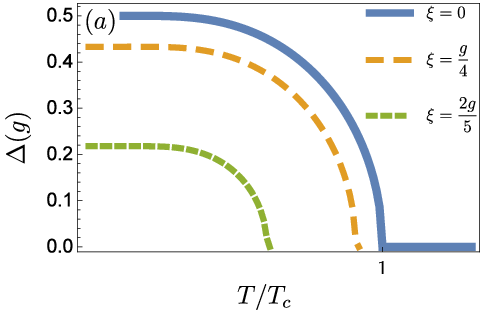
In the case $\omega_{\mathbf{q}}\gg T$, using $V(\mathbf{q})\simeq-g\delta(q)$ yields a separate (transcendental) equation $2E_{\mathbf{k}}=g\tanh\left(\frac{E_{\mathbf{k}}}{2T}\right)$ for each $E_{\mathbf{k}}$. At the Fermi surface the critical temperature is given by $T_{c}(\mathbf{k}_{F})=g/4$, and at $T=0$ the gap function is [32]

A general solution for $\Delta(\mathbf{k})$, as a function of $T$ and $\xi_{\mathbf{k}}$ is shown in Fig. 2 (a).

As a comparison to these results, one can consider the opposite regime, of interaction that is momentum independent $V(\mathbf{q})\simeq-g$. In the case $\omega_{\mathbf{q}}\gg T$, the momentum integral would diverge and the standard procedure, introducing a cutoff $\omega_{D}$, results in $T_{c}=\omega_{D}e^{-1/gN(0)}$. In the case of Eq. (8) the momentum integral does not diverge and can be done analytically, using a typical density of states. The resulting gap function is non zero only for large temperature. A physical interpretation of this scenario is an interesting question, which we do not address in this work.

Discussion. The state described by Eq. (10) has some similarities to the BCS case. The density of states $N(\xi)\propto\Theta(g-2\left|\xi\right|)(\partial\xi_{\mathbf{k}}/\partial\mathbf{k}|_{\xi_{\mathbf{k}}=\xi})^{-1}$ has a gap of $E_{g}=g=4T_{c}$ but no square root singularity. The ratio $E_{g}/T_{c}$ differs by a factor of 1.14 from the BCS result, coming from the lack of integration over momentum/energy. The case of Eq. (9) is rather different. It is valid only in the critical regime of the FE modes, which is mostly $T>0$. It does include a single point in the parameter space with $T=0$, namely the QCP, but at this point $\omega_{0}\rightarrow 0$ and thus $g\rightarrow\infty$. So it is not straight forward to take the limit $T\rightarrow 0$ in order to obtain, for example, the retarded Green’s function, spectral function etc. This might imply that Eq. (9) does not describe any ground state.

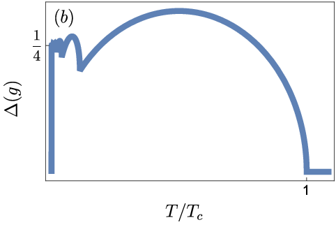
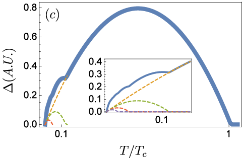
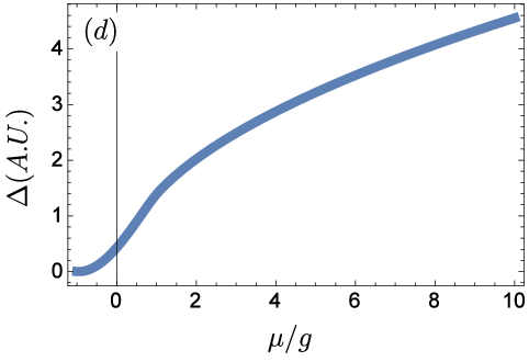
The results in Eqs. (9) and (10) do not depend directly on the density of carriers, in strong contrast to the corresponding expression in BCS theory where $N(0)$ appears in the exponent. This can be attributed to the infinite range of the forward scattering process. The solutions in Eqs. (9) and (10) show possible pairing channels but any observed phenomena, such as persistent current, Meissner effect, Josephson effect etc., might depend on how many channels contribute. In order to study the possible dependence on the doping level and temperature we consider the quantity $\Delta=\sum_{n,\mathbf{k}}\Delta_{n}(\mathbf{k})$, which is plotted in Figs. 2 (c) and (d) as a function of temperature and chemical potential $\mu$ ¹¹ 1 In order to avoid considering the non trivial relation between the Fermi energy and carrier density at finite temperature, we use the grand canonical ensemble, which allows us also to consider negative $\mu$., respectively. The results can be observed experimentally by measuring, for example, the critical current. The qualitative behavior can be inferred at some limits. For a high level of doping $\mu\gg g$ ²² 2 We compare $\mu$ to $g$, so the regime of a high doping level here can correspond to a low level in other contexts and in any case should not be associated with the vanishing SC at increased doping (the other side of the SC dome) we have $\Delta\propto N(0)(T_{c}^{2}-T_{2})$ in the case of Eq. (10) and

in the case of Eq. (9), where in both cases $T_{c}\propto g$. For a low level of doping $\mu\ll g$ we have, in 3 dimensions, $\Delta\propto E_{F}/T_{c}+1$, which implies SC does not vanish for $\mu=0$ and even for $\mu<0$, i.e. an insulator. This result is quite generic, since for $g>-\mu>0$ it can be energetically favored to excite a pair of carriers and allow them to form a bound state. However, this might require extremely strong coupling and low temperature.

The pairing mechanism introduced in this work has the double benefit of being derived from a microscopic model and resulting in unique features that can be experimentally observed. While relying on a physical picture that is different from BCS, this theory still possesses a major advantage of BCS, namely it is analytically tractable. The concrete connection between QCP and SC can be employed as a tool for a theoretical analysis in a wide range of systems. The results might be used to explain pre-pairing observations or the pseudo-gap phenomenon.

Acknowledgments I would like to thank J. M. Edge, T. Kvorning, T. H. Hansson, S. Pershoguba and A.V. Balatsky for helpful discussions. Parts of the results presented in this paper were obtained in collaboration with C. Triola and E. Langmann.

References

- [1] J. Bardeen, L. N. Cooper, and J. R. Schrieffer, Phys. Rev. 108, 1175 (1957).
- [2] D. Eagles, R. Tainsh, and C. Andrikidis, Physica C: Superconductivity 157, 48 (1989).
- [3] X. Lin, Z. Zhu, B. Fauqué, and K. Behnia, Phys. Rev. X 3, 021002 (2013).
- [4] J. Lee, F. Schmitt, R. Moore, S. Johnston, Y.-T. Cui, W. Li, M. Yi, Z. Liu, M. Hashimoto, Y. Zhang, et al., Nature 515, 245 (2014).
- [5] N. Reyren, S. Thiel, A. Caviglia, L. F. Kourkoutis, G. Hammerl, C. Richter, C. Schneider, T. Kopp, A.-S. Rüetschi, D. Jaccard, et al., Science 317, 1196 (2007).
- [6] J. T. Haraldsen, P. Wölfle, and A. V. Balatsky, Phys. Rev. B 85, 134501 (2012).
- [7] D. M. Eagles and P. Lalousis, Journal of Physics C: Solid State Physics 17, 655 (1984).
- [8] D. M. Eagles, Phys. Rev. 145, 645 (1966).
- [9] J. T. Devreese, S. N. Klimin, J. L. M. van Mechelen, and D. van der Marel, Phys. Rev. B 81, 125119 (2010).
- [10] A. G. Swartz, H. Inoue, T. A. Merz, Y. Hikita, S. Raghu, T. P. Devereaux, S. Johnston, and H. Y. Hwang, Proceedings of the National Academy of Sciences 115, 1475 (2018b).
- [11] V. Martelli, J. L. Jiménez, M. Continentino, E. Baggio-Saitovitch, and K. Behnia, Phys. Rev. Lett. 120, 125901 (2018).
- [12] G. Cheng, M. Tomczyk, S. Lu, J. P. Veazey, M. Huang, P. Irvin, S. Ryu, H. Lee, C.-B. Eom, C. S. Hellberg, et al., Nature 521, 196 (2015).
- [13] J. F. Schooley, W. R. Hosler, and M. L. Cohen, Phys. Rev. Lett. 12, 474 (1964).
- [14] Y. Takada, Journal of the Physical Society of Japan 49, 1267 (1980).
- [15] D. van der Marel, J. L. M. van Mechelen, and I. I. Mazin, Phys. Rev. B 84, 205111 (2011).
- [16] L. P. Gor’kov, Proceedings of the National Academy of Sciences 113, 4646 (2016).
- [17] J. Ruhman and P. A. Lee, Physical Review B 94, 224515 (2016).
- [18] L. P. Gor’kov, arXiv preprint arXiv:1610.02062 (2016).
- [19] J. M. Edge, Y. Kedem, U. Aschauer, N. A. Spaldin, and A. V. Balatsky, Phys. Rev. Lett. 115, 247002 (2015).
- [20] Y. Kedem, J.-X. Zhu, and A. V. Balatsky, Phys. Rev. B 93, 184507 (2016).
- [21] A. Stucky, G. Scheerer, Z. Ren, D. Jaccard, J.-M. Poumirol, C. Barreteau, E. Giannini, and D. van der Marel, Scientific Reports 6 (2016).
- [22] C. W. Rischau, X. Lin, C. P. Grams, D. Finck, S. Harms, J. Engelmayer, T. Lorenz, Y. Gallais, B. Fauqué, J. Hemberger, et al., Nature Physics 13, 643 (2017).
- [23] K. Dunnett, A. Narayan, N. Spaldin, and A. Balatsky, arXiv preprint arXiv:1712.08368 (2017).
- [24] S. Rowley, C. Enderlein, J. F. de Oliveira, D. Tompsett, E. B. Saitovitch, S. Saxena, and G. Lonzarich, arXiv preprint arXiv:1801.08121 (2018).
- [25] Y. Wang, A. Abanov, B. L. Altshuler, E. A. Yuzbashyan, and A. V. Chubukov, Phys. Rev. Lett. 117, 157001 (2016).
- [26] S.-G. Jung, S. Seo, S. Lee, E. D. Bauer, H.-O. Lee, and T. Park, Nature communications 9, 434 (2018).
- [27] S. Sachdev, Quantum Phase Transitions (Cambridge University Press, 2011).
- [28] S. Suzuki, J.-i. Inoue, and B. K. Chakrabarti, Quantum Ising Phases and Transitions in Transverse Ising Models, Lecture Notes in Physics, Vol. 862 (Springer Berlin Heidelberg, 2013).
- [29] G. D. Mahan, Many-particle physics, 3rd ed. (Plenum, New York, 2000).
- [30] G. Eliashberg, Sov. Phys. JETP 11, 696 (1960).
- [31] A. Migdal, Sov. Phys. JETP 7, 996 (1958).
- [32] K. Yang and S. L. Sondhi, Phys. Rev. B 62, 11778 (2000).
- [33] G. Varelogiannis, A. Perali, E. Cappelluti, and L. Pietronero, Phys. Rev. B 54, R6877 (1996).
- [34] G. Santi, T. Jarlborg, M. Peter, and M. Weger, Physica C: Superconductivity 259, 253 (1996).
- [35] S. Johnston, I. M. Vishik, W. S. Lee, F. Schmitt, S. Uchida, K. Fujita, S. Ishida, N. Nagaosa, Z. X. Shen, and T. P. Devereaux, Phys. Rev. Lett. 108, 166404 (2012).
- [36] Y. Wang, L. Rademaker, E. Dagotto, and S. Johnston, Phys. Rev. B 96, 054515 (2017).
- [37] L. Rademaker, Y. Wang, T. Berlijn, and S. Johnston, New Journal of Physics 18, 022001 (2016).
- [38] A. Aperis, P. Kotetes, G. Varelogiannis, and P. M. Oppeneer, Phys. Rev. B 83, 092505 (2011).
- [39] In order to avoid considering the non trivial relation between the Fermi energy and carrier density at finite Temperature, we use the grand canonical ensemble, which allow us also to consider negative .
- [40] We compare to , so the regime of a high doping level here can corresponds to a low level in other contexts and in any case should not be associated with the vanishing SC at increased doping (the other side of the SC dome).
Appendices
A The model
Our system comprised of itinerant electrons and electric dipoles that are the source of possible ferroelectricity. The Hamiltonian of the combined system is where , , and are the Hamiltonians for the electrons, the dipoles, their interaction and the direct electron-electron Coulomb interaction. We include here for completeness, even tough it is not included in the main text. The coulomb repulsion lessen superconductivity but has no qualitative effect and including in make the expressions more cumbersome.
The Hamiltonian for a single mode and its coupling to the electrons were derived in the main text. Here we keep the sum over modes throughout the derivation. As mentioned in the main text the modes are assumed to have no interaction between the different directions. In each unit cell , reside three pseudo-spins representing the polarization, i.e. an electric dipole, in the , and directions. Do not confuse the index , which refer to the spatial direction, with the pseudo-spin index referring to different Pauli matrices. The assumption that different modes do not interact means the polarization in one direction, say , does not depend on the polarization in another, say , so we do not have term such as .
The real space Hamiltonians are given by
- [1] R. Roussev and A. J. Millis, Phys. Rev. B 67, 014105 (2003).
- [2] E. Courtens, G. Coddens, B. Hennion, B. Hehlen, J. Pelous, and R. Vacher, Physica Scripta 1993, 430 (1993).
- [3] J. Hemberger, P. Lunkenheimer, R. Viana, R. Böhmer, and A. Loidl, Phys. Rev. B 52, 13159 (1995).