Compassionately Conservative Balanced Cuts for Image Segmentation

The Normalized Cut (NCut) graph partitioning cost function was first introduced over two decades ago to tackle the perceptual grouping problem [18, 19], and its approximate minimization via continuous relaxation into a generalized eigenvector problem has emerged as one of the fundamental techniques of data clustering [13].

The key observation that motivated the normalization of graph cut cost functions is that when graph partitioning is performed by minimizing the sum of the weights of edges that are cut (the Cut cost), the resulting partitions will be unbalanced; vertices that are weakly connected to the rest of the graph are likely to be separated to form singleton partitions, while the rest of the graph vertices are likely to remain in large partitions. Normalizing the cut cost by the degrees of each partition (NCut [18, 19]), the size of each partition (Average Cut [17]), or the minimum of the size of each partition and its complement (Ratio or Cheeger Cut [6]) yield balanced partitions that have similar total degree or size when minimized.

Is it possible that these types of normalization go too far? Consider the example of Figure 1, in which we wish to partition the toy graph into two subgraphs. This graph (1(a)) contains seven vertices and nine edges; all but two of the edges have unit weight, and the two indicated edges have weight $\alpha/2$ for $\alpha\in\left(0,1\right)$. Since $\alpha<1$, the degree of the vertex sharing these two edges is guaranteed to be smaller than the degree of any other vertex in the graph. Hence, as shown in (1(b)), minimizing the Cut cost will separate that weakly-connected vertex from the rest of the graph. Minimizing the NCut cost creates a more balanced partitioning as shown in (1(c)); however, this partitioning will always have a lower-cost NCut than removing the weakly-connected vertex, even when $\alpha$ is infinitesimally small. Perhaps the Ratio Cut (RCut) is a better choice: for this graph, $\alpha=2/3$ is a critical value above which (1(c)) minimizes the RCut cost, and below which (1(b)) yields the minimum. But is there really anything special about $\alpha=2/3$?

If this graph represented an image to be segmented, one would want to use ground-truth segmentation maps from training images to suggest an optimal critical value for $\alpha$, above which the more “balanced” partitioning is desired, and below which the weakly-connected vertex should be separated. The ground truth might dictate that even the Ratio Cut cost provides too much normalization, or instead, that it does not provide enough.

One potential idea is to use the infinite families of balanced cost functions defined by Bühler and Hein [4] and indexed by a parameter $p\in\left(1,\infty\right)$. We refer to these families as the Bühler-Hein $p$-Normalized ($\textrm{BHN}_{p}$) and the Bühler-Hein $p$-Ratio ($\textrm{BHR}_{p}$) Cuts. $\textrm{BHN}_{p}$ is equivalent to NCut for $p=2$ and the Normalized Cheeger (NCh) Cut as $p\rightarrow 1^{+}$, and $\textrm{BHR}_{p}$ is equivalent to RCut for $p=2$ and the Ratio Cheeger (RCh) Cut as $p\rightarrow 1^{+}$, so both families of cut costs can be thought of as interpolating between different normalization factors. However, as shown in Fig. (2), when we minimize $\textrm{BHN}_{p}$ Cut and $\textrm{BHR}_{p}$ Cut for the graph in Fig. (1), there are substantial ranges of $\alpha$ for which no value of $p$ will allow a bifurcation between solutions.

In this paper, we show that although the Bühler-Hein costs provide a mechanism for interpolating between Normalized (or Ratio) Cuts and Normalized (or Ratio) Cheeger Cuts, they do not provide a path for interpolating all the way to the unnormalized Cut cost. However, a different set of infinite families of balanced cost functions can be constructed that do enable such interpolation. Our proposed families are called the Compassionately Conservative Normalized (CCN) Cut and the Compassionately Conservative Ratio (CCR) Cut. Both are indexed by a parameter $\tau\in\left(0,\infty\right)$; $\textrm{CCN}_{\tau}$ is equivalent to NCut for $\tau=2$ and the unnormalized Cut cost for $\tau=0$, and $\textrm{CCR}_{\tau}$ is equivalent to RCut for $\tau=2$ and the unnormalized Cut cost for $\tau=0$. As we can see from Fig. (3), when we minimize $\textrm{CCN}_{\tau}$ and $\textrm{CCR}_{\tau}$ for the graph in Fig. (1), different ranges of $\tau$ can be selected that will allow a bifurcation between solutions for any value of $\alpha$.

This paper makes four novel contributions to graph partitioning in computer vision:

• •

  presenting Compassionately Conservative Balanced (CCB) Cuts: families of cut costs that enable normalizations ranging from Normalized/Ratio Cuts to unnormalized Cuts and can be naturally extended to $k$-way partitionings with $k>2$;

• •

  presenting a continuous relaxation of CCB Cut minimization and illuminating its connection to computing Piecewise Flat Embeddings (PFE) [23];

• •

  presenting an efficient algorithm for solving the relaxed problem via minimizing a succession of reweighted Rayleigh quotients (IRRQ); and

• •

  demonstrating empirical advantages of the CCB Cut costs and the IRRQ minimization algorithm for the application of image segmentation.

Consider an undirected weighted graph $\mathcal{G}=\left(V,E\right)$ that we wish to partition into two disjoint subgraphs $\mathcal{G}_{i}=\left(V_{i},E_{i}\right)$, $i=1,2$, by removing the edges connecting $V_{1}$ and $V_{2}$. A standard cost of partitioning $\mathcal{G}$ is the Cut cost, defined as the total weight of the edges that have been removed:

where the vertex set $V=\left\{v_{1},v_{2},\cdots,v_{n}\right\}$, and $\mathbf{W}$ is the weighted adjacency matrix (or affinity matrix) of $\mathcal{G}$.

Minimizing the Cut cost is undesirable, however, as it can often yield partitionings that simply disconnect one vertex from the rest of the graph [21]. More balanced partitions emerge if the Cut cost is normalized by some function of the total sizes or total degrees (volumes) of the subgraphs. Such balanced cut costs can be expressed generally by:

where $\Theta\!\left(V_{1},V_{2}\right)$ is a symmetric function that decreases with increasing differences in the sizes or degrees of $V_{1}$ and $V_{2}$. A variety of balanced cut costs have been proposed in the literature, including the Normalized Cut [18, 19], Average Cut [17], Ratio Cut [7, 9], and Normalized and Ratio Cheeger Cuts [4, 6].

In Theorem 4.1 of [4], Bühler and Hein show that there exists an infinite family of balanced cut costs that contains Normalized, Average, Ratio, and Cheeger Cuts. If we consider the following function:

for $p>1$ and $v\in\left(0,1\right)$, then $\textrm{BCut}\!\left(V_{1},V_{2}\right)$ with $\Theta\!\left(V_{1},V_{2}\right)=\Phi_{p}\!\left(\left|V_{1}\right|\!/\!\left|V\right|\right)$ is the aforementioned $\textrm{BHR}_{p}$ Cut, and it approaches the Ratio Cheeger Cut as $p\rightarrow 1^{+}$ and equals the Average/Ratio Cuts for $p=2$. If $\Theta\!\left(V_{1},V_{2}\right)=\Phi_{p}\!\left(\textrm{Vol}\!\left(V_{1}\right)\!/\textrm{Vol}\!\left(V\right)\right)$, $\textrm{BCut}\!\left(V_{1},V_{2}\right)$ is the $\textrm{BHN}_{p}$ Cut, and it approaches the Normalized Cheeger Cut as $p\rightarrow 1^{+}$ and equals the Normalized Cut for $p=2$. (The volume of a subgraph is defined as $\textrm{Vol}\!\left(V_{\ell}\right)=\sum_{v_{j}\in V_{\ell}}{d_{j}}$, where $d_{j}=\sum_{m}{w_{j,m}}$ is the degree of vertex $v_{j}$.) Note that this is a rescaling of the balanced cut costs in [4], defined so that the maximum value of $\Theta\!\left(V_{1},V_{2}\right)$ is always unity.

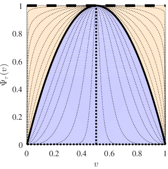
In addition to providing a way to interpolate between Cheeger Cuts and Normalized/Ratio Cuts for $1<p<2$, (3) enables cut costs with normalizations that are slightly more conservative (closer to unity) than Normalized/Ratio Cuts by selecting $p>2$. It is straightforward to show this by noting that:

and so $1>\Phi_{\infty}\!\left(v\right)>\Phi_{2}\!\left(v\right)$ for all $v\in\left(0,1\right)$, $v\neq 1/2$, which can be seen in the left side of Figure 4.

The behavior of (3) as $p\rightarrow\infty$ suggests that there is room to define even more conservative normalization functions. We do so in this paper by considering the following transformation of $\Phi_{p}\!\left(v\right)$:

where $\tau=2/\!\left(p-1\right)$. (The reason for switching parametrizations from $p$ to $\tau$ will be addressed at the end of Section 3.) Clearly $\Psi_{2}\!\left(v\right)=\Phi_{2}\!\left(v\right)$, and so Normalized/Ratio Cuts arise from employing (5) in place of (3) for $\tau=2$. More interestingly, however, is that $\Psi_{0}\!\left(v\right)=1$, and so for $0<\tau<2$, defining $\textrm{BCut}\!\left(V_{1},V_{2}\right)$ with $\Theta\!\left(V_{1},V_{2}\right)=\Psi_{\tau}\!\left(\left|V_{1}\right|\!/\!\left|V\right|\right)$ or $\Psi_{\tau}\!\left(\textrm{Vol}\!\left(V_{1}\right)\!/\textrm{Vol}\!\left(V\right)\right)$ provides a way to interpolate between Normalized/Ratio Cuts and Cuts with no normalization at all. This behavior of increasing $\Psi_{\tau}\!\left(v\right)$ as $\tau\rightarrow 0^{+}$ can be seen in the right side of Figure 4.

Of pedagogical interest is that $\lim_{\tau\rightarrow\infty}{\Psi_{\tau}\!\left(v\right)}=\delta\!\left(v-1/2\right)$, and so as $\tau\rightarrow\infty$, employing (5) to define $\Theta\!\left(V_{1},V_{2}\right)$ would yield balanced cut costs that diverge whenever the sizes or degrees of $V_{1}$ and $V_{2}$ are unequal. Since our interest in this paper is to explore the impact of cut costs having more conservative normalizations than Normalized/Ratio Cuts, we will restrict our attention to the use of $\Psi_{\tau}\!\left(v\right)$ for $\tau\in\left(0,2\right)$.

In addition to enabling a greater range of conservative normalizations, the use of (5) in place of (3) yields an added benefit: the resulting Balanced Cut costs can be directly extended to form costs of partitionings into $k>2$ subgraphs. (As discussed in [4], it is not obvious whether such a direct extension to the Bühler-Hein cut costs exists.) If we now consider that we wish to partition $\mathcal{G}$ into $k$ disjoint subgraphs $\mathcal{G}_{i}=\left(V_{i},E_{i}\right)$, $i=1,2,\ldots,k$, then an unbalanced way to measure the cost of the partitioning is the multiway cut cost, defined in terms of pairwise cut costs as:

The family of multiway balanced cut costs that we propose is described generally by the Compassionately Conservative Balanced Cut:

where $\bm{\pi}=\left[\pi_{1},\ldots,\pi_{n}\right]^{\mathbf{T}}$ is a user-defined vector of positive weights. If $\bm{\pi}=\mathbf{1}_{n}$, then $\sum_{v_{j}\in V_{\ell}}{\pi_{j}}=\left|V_{\ell}\right|$, and we refer to (7) as the Compassionately Conservative Ratio Cut ($\textrm{CCR}_{\tau}$). If $\bm{\pi}=\mathbf{d}$ (the degree vector), then $\sum_{v_{j}\in V_{\ell}}{\pi_{j}}=\textrm{Vol}\!\left(V_{\ell}\right)$, and we refer to (7) as the Compassionately Conservative Normalized Cut ($\textrm{CCN}_{\tau}$). With some algebraic manipulation, it is straightforward to see that (7) is a generalization of (2); when $k=2$, (7) reduces to (2) with $\Theta\!\left(V_{1},V_{2}\right)=\Psi_{\tau}\!\left(\sum_{v_{j}\in V_{1}}{\pi_{j}}\middle/\sum_{v_{j}\in V}{\pi_{j}}\right)$. Furthermore, (7) generalizes multiclass cut costs presented in the research literature; $\textrm{CCB}_{2}$, $\textrm{CCR}_{2}$, and $\textrm{CCN}_{2}$ are scaled versions of the Multiclass Penalized Cut [24], the Multiclass Ratio Cut [20], and the Multiclass Normalized Cut [22, 20], respectively, and so choosing $\tau\in\left(0,2\right)$ generates Multiclass Balanced Cut costs that interpolate between (6) and any of these previously developed costs.

As with many balanced cut costs, minimizing the CCB Cut is NP-hard. However, we can formulate a continuous relaxation of $\textrm{CCB}_{\tau}$ for all $\tau>0$. Unfortunately, the spectral clustering relaxation of $\textrm{BHN}_{p}$ and $\textrm{BHR}_{p}$ in terms of the second eigenvector of the graph $p$-Laplacian [4] is of no help; it is only tight as $p\rightarrow 0^{+}$ (and therefore not for $\tau\in\left(0,2\right)$), and furthermore, CCB Cuts are not even members of the Bühler-Hein family of cuts except for when $\tau=p=2$. Hence, we must identify a different relaxation.

To do so, we first reformulate $\textrm{CCB}_{\tau}$ to express it in terms of an $n\times k$ indicator matrix $\mathbf{X}$ so that $X_{i,j}=1$ if $v_{i}\in V_{j}$ and $X_{i,j}=0$ otherwise. If $\mathbf{x}_{i}$ is the $i^{\textrm{th}}$ column of $\mathbf{X}$, then $\sum_{v_{j}\in V_{i}}{\pi_{j}}$ can be written in terms of the diagonal matrix $\bm{\Pi}=\textrm{diag}\!\left(\bm{\pi}\right)$ as $\mathbf{x}_{i}^{\mathbf{T}}\bm{\Pi}\mathbf{x}_{i}$, and the pairwise cut cost between $V_{i}$ and $V\backslash V_{i}$ can be written as $\textrm{Cut}\!\left(V_{i},V\backslash V_{i}\right)=\mathbf{x}_{i}^{\mathbf{T}}\mathbf{W}\left(\mathbf{1}-\mathbf{x}_{i}\right)=\mathbf{x}_{i}^{\mathbf{T}}\mathbf{d}-\mathbf{x}_{i}^{\mathbf{T}}\mathbf{W}\mathbf{x}_{i}=\mathbf{x}_{i}^{\mathbf{T}}\mathbf{D}\mathbf{x}_{i}-\mathbf{x}_{i}^{\mathbf{T}}\mathbf{W}\mathbf{x}_{i}=\mathbf{x}_{i}^{\mathbf{T}}\mathbf{L}\mathbf{x}_{i}$, where $\mathbf{L}=\mathbf{D}-\mathbf{W}$. This allows us to express (7) as:

Minimizing (7) is equivalent to minimizing (8) subject to the constraint that $\mathbf{X^{T}X}$ is positive diagonal, which ensures that none of the $V_{i}$’s will collapse to the empty set.

To guide us towards an appropriate $\textrm{CCB}_{\tau}$ relaxation, we first consider how the Multiclass Penalized Cut ($\textrm{CCB}_{2}$) can be relaxed. Using an argument similar to Yu and Shi [22], we see that if $\mathbf{Y}=\mathbf{X}\!\left(\mathbf{X^{T}\bm{\Pi}X}\right)^{-1/2}$, then $\mathbf{Y^{T}\bm{\Pi}Y}=\mathbf{I}$ and (7) is equivalent to a scalar multiple of $\textrm{tr}\!\left(\mathbf{Y^{T}LY}\right)$. Hence, the solution to minimizing a relaxed version of $\textrm{CCB}_{2}$ is $\mathbf{\tilde{Y}}=\mathbf{UQ}$, where $\mathbf{U}$ is the $n\!\times\!k$ matrix whose columns are the orthonormal eigenvectors $\mathbf{u}_{2}$, $\ldots$, $\mathbf{u}_{k+1}$ corresponding to the smallest nontrivial eigenvalues of $\bm{\Pi}^{-1/2}\mathbf{L}\bm{\Pi}^{-1/2}$, and $\mathbf{Q}$ is an arbitrary $k\!\times k$ orthogonal matrix. The optimal solution $\mathbf{\tilde{X}}$ to (7) with $\tau=2$ can then be approximated by $k$-means clustering [15], nonmaximal suppression [22] or Procrustean rounding [24] on $\mathbf{\tilde{Y}}$.

Note that if we define $\mathbf{\hat{y}}_{i}$ to be the transpose of the $i^{\textrm{th}}$ row of $\mathbf{Y}$, then minimizing the relaxed version of $\textrm{CCB}_{2}$ is equivalent to solving the constrained minimization problem:

which, when $\bm{\pi}=\mathbf{d}$, is identical to the Laplacian Eigenmaps (LE) problem [3] for computing embeddings of data that are assumed to lie on a manifold. The balance constraint $\mathbf{Y^{T}\bm{\Pi}1}=\mathbf{0}$ is necessary to avoid eigenvectors of $\bm{\Pi}^{-1/2}\mathbf{L}\bm{\Pi}^{-1/2}$ corresponding to the trivial eigenvalue.

Turning our attention now to the more general case where $\tau>0$, if we define $\alpha_{\ell}=\left(\sum_{i}{\pi_{i}x_{i,\ell}^{2}}\right)^{-1/2}$ for $\ell=1,\ldots,k$, and we note that $\left(\mathbf{X^{T}\bm{\Pi}X}\right)^{-1/2}=\textrm{diag}\!\left(\bm{\alpha}\right)$, we can write:

Hence, the relaxation of (8) is obtained by dropping the condition that $\mathbf{Y}=\mathbf{X}\!\left(\mathbf{X^{T}\bm{\Pi}X}\right)^{-1/2}$ and solving the constrained minimization problem:

Note that the balance constraint $\mathbf{Y^{T}\bm{\Pi}1}=\mathbf{0}$ is only necessary for the case $\tau=2$.

Remarkably, in the special case where $\bm{\pi}=\mathbf{d}$ and $\tau=1$, (11) is exactly the Piecewise Flat Embedding (PFE) problem [23], whose solution is an embedding in which the data are naturally clustered due to the promotion of sparsity in the differences between rows of $\mathbf{Y}$. It is for this reason that we choose to parametrize CCB Cuts in terms of $\tau$ and not $p$: solutions to the relaxed versions of $\textrm{CCB}_{\tau}$ for $\tau\in\left(0,1\right]$ can be expected to be piecewise constant, consistent with the sparse nature of solutions to $\ell_{\tau}$-minimization problems for $\tau\in\left(0,1\right]$.

While (11) with $\tau=2$ has a solution that can be written in terms of the eigenvectors corresponding to the smallest $k$ nontrivial eigenvalues of $\bm{\Pi}^{-1/2}\mathbf{L}\bm{\Pi}^{-1/2}$, no analytical form of the solution is known for $\tau\neq 2$. In [23], Yu et al. proposed approximating the solution to (11) with $\tau=1$ via the Splitting Orthogonality Constraint (SOC) algorithm [14], which requires an initial estimate of $\mathbf{Y}$ and performs a nested iteration with parameters at each level that must be tuned. While it is possible to partially generalize this approach to handle (11) with $\tau>1$, $\mathcal{J}_{\tau}\!\left(\mathbf{Y}\right)$ is non-convex for $\tau\in\left(0,1\right)$, and so the SOC algorithm is not applicable in this regime. Furthermore, even in the regime in which it is applicable, the use of splitting in the algorithm formulation means that the solutions will not strictly satisfy the orthogonality constraint $\mathbf{Y^{T}DY}=\mathbf{I}$.

Here, we propose an alternative algorithm for solving (11) that can be applied for all $\tau\in\left(0,2\right]$, that does not require an initial estimate of $\mathbf{Y}$, and that does strictly satisfy the orthogonality constraint. Our alternative algorithm is motivated from the Iteratively Reweighted Least Squares (IRLS) algorithms commonly used to solve $\ell_{1}$-minimization problems [8]. In IRLS, $\ell_{1}$-minimization is performed by iteratively solving a succession of weighted least-squares ($\ell_{2}$-minimization) problems, with the weights updated at each iteration so as to decrease the impact of large residual errors. IRLS algorithms do require initialization, but it is the weights that must be initialized as opposed to the solution. Weights are typically initialized to unity (although they can be initialized differently by an expert user), and in specific cases [8], IRLS algorithms have provable convergence guarantees.

In our relaxed problem (11), the presence of the orthogonality constraint renders IRLS algorithms invalid. However, solutions to (11) can be approximated by iteratively solving a series of constrained weighted $\ell_{2}$-minimization problems, each of the form:

where $\mathbf{\Gamma}$ is the $n\times n$ matrix of weights (with entries $\gamma_{i,j}$) that is updated at each iteration in a manner similar to IRLS.

To establish a connection between (11) and (12), we first eliminate the balance constraint from (12) using the result of the following Lemma, which is proved in Appendix C:

Using this Lemma allows us to solve (12) by first solving:

and then computing $\mathbf{Y}=\bm{\aleph}\!\left(\mathbf{\hat{G}}\right)$.

An analogy to IRLS suggests that under the assumption that component-wise differences in the embedding do not vanish, the best choice of weights for (12) would be $\gamma_{i,j}=\left\|\mathbf{\hat{y}}_{i}^{\ast}-\mathbf{\hat{y}}_{j}^{\ast}\right\|^{\tau}_{\tau}/\left\|\mathbf{\hat{y}}_{i}^{\ast}-\mathbf{\hat{y}}_{j}^{\ast}\right\|^{2}_{2}$ for $i\neq j$, where $\mathbf{Y}^{\ast}$ is the solution to (11). This choice of weights would yield $\mathcal{J}_{2}^{\mathbf{\Gamma}}\!\left(\mathbf{Y}^{\ast}\right)=\mathcal{J}_{\tau}\!\left(\mathbf{Y}^{\ast}\right)$. In practice, however, $\mathbf{Y}^{\ast}$ is unknown, and many of the component-wise differences in the embedding will vanish. Hence, we propose using regularized weights as suggested in [8]:

and we update $\varepsilon$ according to the schedule prescribed by [8], which suggests:

where $r\!\left(\mathbf{Y}\right)_{\kappa}$ is the $\kappa^{\textrm{th}}$ largest element of $\left\{w^{1/2}_{i,j}\!\left\|\mathbf{\hat{y}}_{i}-\mathbf{\hat{y}}_{j}\right\|_{2},\forall i,j=1,\ldots,n\right\}$.

Combining the steps of solving (12) and updating (14)–(15) into a sequence of iterations yields Algorithm 1 for computing the solution to (11). Since (12) is equivalent to (13), and (13) can be transformed into an unconstrained minimization of a Rayleigh Quotient, we term this algorithm Iteratively Reweighted Rayleigh Quotient (IRRQ) Minimization.

Unlike SOC, IRRQ requires tuning of only a single hyperparameter $\kappa$, it can be used for any $\tau\in\left(0,2\right)$, and it guarantees a solution in which the orthogonality constraint is strictly enforced. Furthermore, IRRQ does not require a preprocessing step to estimate an initial clustering; rather, only the weights $\gamma_{i,j}$ must be initialized, and they can all be initialized to unity. Interestingly, this initialization is equivalent to implicitly using an initial clustering that corresponds to the solution of the relaxed NCut problem. This is because $\mathcal{J}_{2}^{\mathbf{11^{T}}}\!\left(\mathbf{Y}\right)$ is equivalent to the LE objective function $\mathcal{J}_{2}\!\left(\mathbf{Y}\right)$ in (9). If different initializations are desired, for instance, by computing an initial embedding $\mathbf{Y}^{\left(0\right)}$ using a Gaussian Mixture Model as in [23], these can be incorporated by setting the initial weights to be $\gamma_{i,j}^{\left(0\right)}=\left\|\mathbf{\hat{y}}_{i}^{\left(0\right)}-\mathbf{\hat{y}}_{j}^{\left(0\right)}\right\|_{\tau}^{\tau}/\left\|\mathbf{\hat{y}}_{i}^{\left(0\right)}-\mathbf{\hat{y}}_{j}^{\left(0\right)}\right\|_{2}^{2}$ or $\gamma_{i,j}^{\left(0\right)}=\left[w_{i,j}\!\left\|\mathbf{\hat{y}}_{i}^{\left(0\right)}-\mathbf{\hat{y}}_{j}^{\left(0\right)}\right\|_{2}^{2}+\varepsilon_{0}^{2}\right]^{-1+\tau/2}$.

To investigate the performance of CCB Cuts for image segmentation, we segment the 200 test images in the BSDS500 dataset [1], each of which has a variety of manually-labeled segmentations with different numbers of segments that can be used as ground truth. We explore three different affinity constructions for each image:

• •

  Lab: a Gaussian kernel on squared Euclidean distances in $\textrm{L}^{*}\textrm{a}^{*}\textrm{b}^{*}$ color space;

• •

  mPb: an exponentiated negative maximum of the multiscale probability of boundary (mPb) using the code provided with the BSDS500 dataset [1]; and,

• •

  PMI: an exponentiated version of a statistic related to pointwise mutual information (PMI) used in crisp boundary detection [12].

We use a $10$-pixel radius to define neighborhoods for affinity construction. For efficiency, we downsample each affinity matrix by two scale levels (and subsequently upsample the computed embeddings) using the strategy in [2, 16].

Figure 6 illustrates segmentation results on a BSDS500 test image for both multi-way and hierarchical 2-way segmentation using various types of balanced cuts. Although different segmentations appear to have different numbers of regions, many of the regions are small/singleton, and all segmentation results have the same number of regions. Figure 6 shows how hierarchical 2-way segmentation using CCN Cuts with $\tau=1$ does not exhibit the iterative “chopping” behavior common to hierarchical NCuts minimization.

Compassionately Conservative Balanced Cuts enable normalizations ranging from Normalized/Ratio Cuts to unnormalized Cuts, allowing a tradeoff between generating partitions that are too similar in size/degree and avoiding all singletons. They can be directly applied to the $k$-way partitioning problem for any $k\geq 2$, and their minimization can be relaxed into a problem that can be solved by minimizing a succession of Rayleigh quotients. Image segmentation experiments show that minimizing the CCB Cut yields more accurate results than minimizing NCuts/RCuts and generates regions having greater variability in size/degree.

References

- [1] P. Arbeláez, M. Maire, C. Fowlkes, and J. Malik. Contour detection and hierarchical image segmentation. IEEE Trans. Pattern Analysis and Machine Intelligence, 33(5):898–916, May 2011.
- [2] P. Arbeláez, J. Pont-Tuset, J. Barron, F. Marques, and J. Malik. Multiscale combinatorial grouping. In Proc. Computer Vision and Pattern Recognition, CVPR, pages 328–335, 2014.
- [3] M. Belkin and P. Niyogi. Laplacian eigenmaps for dimensionality reduction and data representation. Neural computation, 15(6):1373–1396, 2003.
- [4] T. Bühler and M. Hein. Spectral clustering based on the graph p-Laplacian. In Proc. International Conference on Machine Learning, ICML, pages 81–88. ACM, 2009.
- [5] T. Bühler, S. S. Rangapuram, S. Setzer, and M. Hein. Constrained fractional set programs and their application in local clustering and community detection. In Proc. International Conference on Machine Learning, ICML, pages 624–632, 2013.
- [6] J. Cheeger. A lower bound for the smallest eigenvalue of the laplacian. In Proceedings of the Princeton Conference in Honor of Professor S. Bochner, pages 195–199, 1969.
- [7] C.-K. Cheng and Y.-C. A. Wei. An improved two-way partitioning algorithm with stable performance. IEEE Trans. Computer-Aided Design of Integrated Circuits and Systems, 10(12):1502–1511, 1991.
- [8] I. Daubechies, R. DeVore, M. Fornasier, and C. S. Güntürk. Iteratively reweighted least squares minimization for sparse recovery. Communications on Pure and Applied Mathematics, 63(1):1–38, 2010.
- [9] L. Hagen and A. B. Kahng. New spectral methods for ratio cut partitioning and clustering. IEEE Trans. Computer-Aided Design of Integrated Circuits and Systems, 11(9):1074–1085, 1992.
- [10] M. Hein and T. Bühler. An inverse power method for nonlinear eigenproblems with applications in 1-spectral clustering and sparse PCA. In Advances in Neural Information Processing Systems, NIPS, pages 847–855, 2010.
- [11] M. Hein and S. Setzer. Beyond spectral clustering - tight relaxations of balanced graph cuts. In Advances in Neural Information Processing Systems, NIPS, pages 2366–2374, 2011.
- [12] P. Isola, D. Zoran, D. Krishnan, and E. H. Adelson. Crisp boundary detection using pointwise mutual information. In Proc. European Conference on Computer Vision, ECCV, pages 799–814. Springer, 2014.
- [13] A. K. Jain. Data clustering: 50 years beyond K-means. Pattern Recognition Letters, 31(8):651–666, 2010.
- [14] R. Lai and S. Osher. A splitting method for orthogonality constrained problems. Journal of Scientific Computing, 58(2):431–449, 2014.
- [15] A. Y. Ng, M. I. Jordan, and Y. Weiss. On spectral clustering: Analysis and an algorithm. In Advances in Neural Information Processing Systems, NIPS, pages 849–856, 2002.
- [16] J. Pont-Tuset, P. Arbeláez, J. T. Barron, F. Marques, and J. Malik. Multiscale combinatorial grouping for image segmentation and object proposal generation. IEEE Trans. Pattern Analysis and Machine Intelligence, 39(1):128–140, 2017.
- [17] S. Sarkar and P. Soundararajan. Supervised learning of large perceptual organization: Graph spectral partitioning and learning automata. IEEE Trans. Pattern Analysis and Machine Intelligence, 22(5):504–525, 2000.
- [18] J. Shi and J. Malik. Normalized cuts and image segmentation. In Proc. Computer Vision and Pattern Recognition, CVPR, pages 731–737, Jun 1997.
- [19] J. Shi and J. Malik. Normalized cuts and image segmentation. IEEE Trans. Pattern Analysis and Machine Intelligence, 22(8):888–905, Aug 2000.
- [20] U. Von Luxburg. A tutorial on spectral clustering. Statistics and computing, 17(4):395–416, 2007.
- [21] Z. Wu and R. Leahy. An optimal graph theoretic approach to data clustering: theory and its application to image segmentation. IEEE Trans. Pattern Analysis and Machine Intelligence, 15(11):1101–1113, Nov 1993.
- [22] S. X. Yu and J. Shi. Multiclass spectral clustering. In Proc. International Conference on Computer Vision, ICCV, pages 313–319, 2003.
- [23] Y. Yu, C. Fang, and Z. Liao. Piecewise flat embedding for image segmentation. In Proc. International Conference on Computer Vision, ICCV, pages 1368–1376, 2015.
- [24] Z. Zhang and M. I. Jordan. Multiway spectral clustering: A margin-based perspective. Statistical Science, 23(3):383–403, 2008.