Shake genus and slice genus
Abstract.
An important difference between high dimensional smooth manifolds and smooth 4-manifolds that in a 4-manifold it is not always possible to represent every middle dimensional homology class with a smoothly embedded sphere. This is true even among the simplest 4-manifolds: obtained by attaching an -framed 2-handle to the 4-ball along a knot in . The -shake genus of records the minimal genus among all smooth embedded surfaces representing a generator of the second homology of and is clearly bounded above by the slice genus of . We prove that slice genus is not an invariant of , and thereby provide infinitely many examples of knots with -shake genus strictly less than slice genus. This resolves Problem 1.41 of [Kir97]. As corollaries we show that Rasmussen’s invariant is not a -trace invariant and we give examples, via the satellite operation, of bijective maps on the smooth concordance group which fix the identity but do not preserve slice genus. These corollaries resolve some questions from [4MK16].
1. Introduction
One of the key differences between smooth 4-manifolds and higher dimensional smooth manifolds is the ability to represent any middle dimensional homology class with a smoothly embedded sphere. For 4-manifolds this is not always possible even in the simplest case: four-manifolds obtained by attaching an -framed 2-handle to the 4-ball along a knot in . We call such a manifold the -trace of . The -shake genus of , denoted , measures this failure to find a sphere representative by recording the minimal genus among smooth embedded generators of the second homology of .
Recall that the slice genus of , denoted , is defined to be the minimal genus of a smooth properly embedded surface such that . When we attach a 2-handle to along , any such can be capped off to a closed surface of the same genus. So we see that for all integers and knots the -shake genus is bounded above by the slice genus. Since is embedded in a restrictive manner ( intersects the cocore of the handle in one point) one might expect that the -shake genus can be strictly less than the slice genus. Indeed for such examples are well-known [Akb77, Lic79, Akb93, AJOT13, CR16]. All of these examples rely on the same proof technique: produce two knots and with diffeomorphic to , then show that . This paper concerns the case .
There are a few issues with using the proof outline to show that there exist such that . A longstanding conjecture of Akbulut and Kirby, Problem 1.19 of [Kir97], held that if the 3-manifolds and obtained by 0-framed Dehn surgery on knots and are homeomorphic, then and are (smoothly) concordant. Since arises naturally as , any attempt to use the argument to show there exist such that must disprove this conjecture along the way. It is a priori possible to show that there exist knots with without exhibiting a counterexample to the Akbulut Kirby conjecture but to do so one would need to demonstrate that there exists a knot with and so that for any smooth embedded minimal genus surface generating there is no description of consisting of only a and handle in which can be isotoped to meet the cocore of the handle transversely in a point. The existence of such a knot seems to be a subtle problem; it is not resolved here.
In 2015 Yasui disproved the Akbulut-Kirby conjecture [Yas15], and it was later demonstrated by A. N. Miller and the author that there exist non-concordant knots with diffeomorphic -traces [MP18]. These results give some evidence that that it might in fact be possible to show that there exist with by producing knots and with diffeomorphic to and .
Some concerns with that outline remain; first, there is a brief classical argument, see [KM78], showing that if a knot shares a 0-trace with a slice knot then is slice. As such, the standard outline cannot be used to show that there exist 0-shake slice knots which are not slice; the existence of such knots remains open. Second, the -surgery of a knot, and hence the -trace, determines fundamental slice genus bounds such as the Tristram-Levine signatures, Casson-Gordon signatures, and signature invariants associated to the filtration of [COT03]. In fact there was only one smooth concordance invariant known not to be a -trace invariant, and that invariant does not give slice genus bounds, see [MP18]. Nevertheless, we have
Theorem 1.1.
There exist infinitely many pairs of knots and such that is diffeomorphic to and .
Corollary 1.2.
There exist infinitely many knots with .
This solves problem 1.41 of [Kir97].
The constructive half of the proof of Theorem 1.1 relies on a reinterpretation of a classical technique of Lickorish [Lic79] and Brakes [Bra80] to produce and with diffeomorphic to . Lickorish and Brakes’ technique can be used to produce all of the knots that have been used to show for in the literature. However, all the knots considered in any of the literature have and and as such cannot be used to prove Theorem 1.1.
With our new perspective (Theorem 2.1) we produce pairs of knots with diffeomorphic 0-traces which a priori should be expected to have large slice genus. In Theorem 2.3 we then give a more restrictive construction allowing us to build such a pair where , surprisingly, has some prescribed small slice genus. This second construction is non-symmetric in and , so one still expects that is large. We give an infinite family where this occurs, as well as several isolated examples. To give lower bounds on we use Rasmussen’s invariant. Hence
Corollary 1.3.
Rasmussen’s invariant is not a 0-trace invariant
This addresses question 12 of [4MK16]. It is still unknown whether Ozsváth-Szabó’s invariant is an invariant of the 0-trace of .
Let denote smooth concordance and knots in be the concordance group. Any pattern in a solid torus a induces a well-defined map by taking where acts on knots by the satellite operation. Since one is interested in understanding one might hope that sometimes induces an automorphism; in fact it unknown whether a satellite operator can ever induce a homomorphism of and it is conjectured that it cannot [SST16]. More generally, one asks what sort of maps on can be obtained via the satellite operation. With an eye toward better understanding , this is in particular an interesting question when attention is restricted to satellite operators with winding number 1.
It has been shown that winding number 1 satellite operators can induce non-surjective maps [Lev16] and interesting bijective maps [GM95][MP18], and that there exist patterns such that but with for some [CFHH13]. It is still unknown whether winding number 1 satellite operators can induce non-injective maps [CR16]. Problem 7 of [4MK16] asked whether there exist winding number one patterns such that but with for some ; we resolve this as a corollary of our main theorem.
Corollary 1.4.
There exist satellite operators such that and such that induces a bijection on but such that does not preserve slice genus.
Satellite operators which induce bijections that fix the identity give candidates for automorphisms of . Motivated by checking whether the examples used to prove Corollary 1.4 are automorphisms, we give a pair of obstructions to a satellite map inducing a homomorphism on . One of the obstructions is given below, the second is somewhat technical to state and is relegated to Section 4. While these obstructions are not particularly difficult and may be known to experts, we cannot find proofs in the literature so we produce them here.
Theorem 1.5.
Let be a winding number pattern and suppose that there exists some knot and additive slice genus bound such that
Then is not a homomorphism.
Corollary 1.6.
The satellite operators used to prove Corollary 1.4 do not induce automorphisms on .
In a similar spirit, we show
Theorem 1.7.
Suppose a pattern induces a homomorphism on . If has winding number 0 then has stable slice genus 0 for all . If has winding number one then has stable slice genus 0 for all .
The only known examples of knots with stable slice genus are the amphichiral knots, which have 2-torsion in . As such, Theorem 1.7 can be read as evidence that winding number 0 and 1 satellite operators never induce interesting homomorphisms. See Section 4 for further discussion.
All manifolds, submanifolds, maps of manifolds and concordances are smooth throughout this work, all homology has integer coefficients and all knots and manifolds are taken to be oriented. We will use to denote diffeomorphic manifolds, to denote isotopic links, and to denote concordant knots. We will assume familiarity with handle calculus, for the details see [GS99].
Acknowledgements
The author previously explored many of these tools and objects in joint work with Allison N. Miller [MP18] and that collaboration, as well as many subsequent insightful conversations, informs this work. Additionally, the author is grateful to Allison for pointing out an error in an early proof of Theorem 1.5 and for comments on a draft of this paper. Conversations with Jeff Meier were clarifying and motivating and we are also grateful to Tye Lidman for helpful conversations.
We would like to acknowledge the developer of the Kirby Calculator [Swe11] which we found helpful and sanity preserving while developing the examples in this work. Finally, the author is hugely grateful to her adviser, John Luecke, for extraordinary generosity with his encouragement, expertise, and time.
The author was partially supported by an NSF GRFP fellowship.
2. Constructing knots with diffeomorphic traces
We begin by constructing pairs of knots with diffeomorphic traces. Theorem 2.1 was motivated by an inside-out take on the well-known dualizable patterns construction.
Let be a three component link with (blue, green, and red) components and such that the following hold: the sublink is isotopic in to the link where denotes a meridian of , the sublink is isotopic to the link , and lk. From we can define an associated four manifold by thinking of as a 1-handle, in dotted circle notation, and and as attaching spheres of 0-framed 2-handles. See Figure 4 for an example of such a handle description. In a moment we will also define a pair of knots and associated to .
Theorem 2.1.
.
Proof.
Isotope to a diagram in which has no self crossings (hence such that bounds a disk in the diagram) and in which is a single point. Slide over as needed to remove the intersections of with . After the slides we can cancel the two handle with attaching circle with the one handle and we are left with a handle description for a 0-framed knot trace; this knot is .
To construct and see , perform the above again with the roles of and reversed. ∎
Remark 2.2.
By modifying the framing hypotheses in Theorem 2.1 this technique can be easily modified to produce knots and with for any integer .
For a link in , define to be the mirror of with its orientation reversed. Two -component links and are said to be strongly concordant if they cobound a smoothly embedded surface in such that is a disjoint union of annuli and and . When we omit the word strongly.


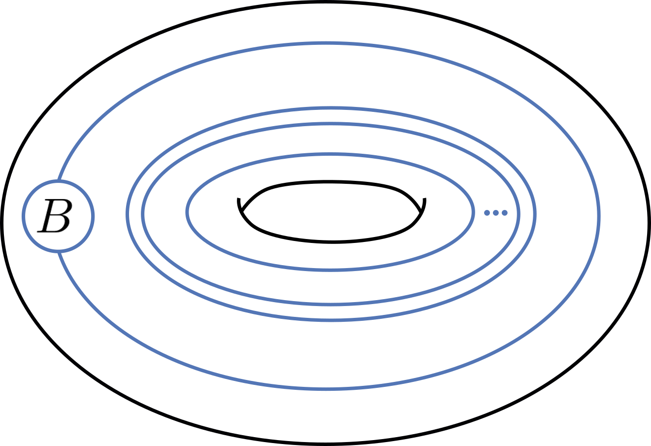
Theorem 2.3.
Proof.
Since is split, there exist finitely many crossing changes of with which change into the link in Figure 1. As such there is a finite sequence of bands of , as in Figure 2, which change into the link in Figure 1. Then there is a diagram of obtained by performing the dual bands to given diagram of ; isotope to this diagram and decorate it with the bands . Then slide across at all points of so that we can cancel the 2-handle with the one handle. We obtain a diagram of decorated with bands, and such that when these bandings of are performed we obtain the link , where is the pattern in Figure 3. Since is slice we obtain that the link is strongly concordant to , hence is concordant to . ∎

Example 2.4.
Let be an integer and be the decorated link on the left hand side of Figure 4, which describes a four manifold , and observe that satisfies the hypotheses of Theorem 2.3. After the indicated slides we obtain a diagram of as the 0-trace of a knot we call . By Theorem 2.3, is concordant to which we see is isotopic to the right-hand trefoil for all .

We then isotope to get a handle diagram for as the 0-trace of a knot we call . See Figure 5.
Remark 2.5.
In Figure 4 we have illustrated bands such that banding along in the left hand diagram changes into a three component link split from , where two components are isotopic to , as in the proof of Theorem 2.3. We also kept track of through the diffeomorphism. In practice neither exhibiting nor keeping track of the bands is necessary; we have included it here to build intuition for the proof of Theorem 2.3 and demonstrate how Theorem 2.3 can be used to give an explicit description of the implied concordance.
The diagram we give of in Figure 4 can certainly be simplified, but since we will only be concerned with up to concordance and we understand by Theorem 2.3, we don’t pursue this. This illustrates the usefulness of Theorem 2.3; if one wants to compare the concordance properties of knots with diffeomorphic traces one can get a tractable pair by choosing so that remains relatively simple (in crossing number perhaps, or whatever is convenient) and since we understand it does not matter if the knot is complicated.

3. Rasmussen’s invariant calculations
In [Kho00], Khovanov introduced a link invariant which takes the form of a bigraded abelian group. We refer to this group as the Khovanov homology , and will sometimes find it convenient to refer to the Poincare polynomial of this group, which is
Later, Lee showed that can be viewed as the page of a spectral sequence which converges to [Lee08] and Rasmussen used this to define an integer valued knot invariant [Ras10]. It will suffice for this work to recall the following properties of .
Theorem 3.1 ([Ras10]).
For any knot in , the following hold:
- (1)
- (2)
The map induces a homomorphism from to .
- (3)
Corollary 3.2 ([Ras10]).
Suppose and are knots that differ by a single crossing change, from a positive crossing in to a negative one in . Then .

Proof of Theorem 1.1.
For a fixed let and be the knots from Example 2.4. By Theorem 2.1 , and as remarked in Example 2.4, for all . For we will bound the slice genus of from below by bounding from below. See Figure 7 for a somewhat reduced diagram of with approximately 40 crossings. We make use of the JavaKh routines, available at [KAT] to compute . These routines produce Poincare polynomial
| (1) |
Remark 3.3.
It is not hard to check that for all . Hence all bounds in the above proof are sharp.
We now produce another isolated example of a pair of knots with and . This example could also be expanded to infinite families as done with Example 2.4, but we do not pursue that here. This and the the knots in Example 2.4 are only special in that they have with reasonably small crossing number, allowing us to compute . We anticipate that Theorem 2.3 can be used to give abundant examples of knots with diffeomorphic traces and distinct slice genera.
Example 3.4.

Let be the decorated link in the left hand side of Figure 8. By Theorems 2.1 and 2.3, gives a handle decomposition for where is concordant to the right hand trefoil. By performing the slides indicated in the left hand side of Figure 8 one obtains a knot with , not pictured. In the right hand side of Figure 8 we give a diagram of a knot with fewer crossings; we claim is isotopic to . The isotopy between the diagram of described and the diagram of given is non-trivial, we provide two options for the careful reader to confirm the existence of an isotopy. First, they can use Snappea [Wee01] to confirm that the diagrams present isotopic knots. Alternatively they can use the Kirby calculator [Swe11] to view the diffeomorphism which we have located on the author’s website [Pic] and can check that this diffeomorphism sends a 0-framed copy of to . We warn that the diffeomorphism is tedious.
Having confirmed that it suffices to compute . As before we rely on the JavaKh routines and item 3 of 3.1. We suppress the output of JavaKh and present the conclusion, which is that . Since one checks that we conclude and .
4. Bijective maps on which do not preserve slice genus, and some satellite homomorphism obstructions
4.1. Definitions and notation
Let be an oriented link in a parametrized solid torus . By the usual abuse of notation, we use to refer to both this map and its image. Define for some , oriented so that is homologous to a non-negative multiple of . We call the (algebraic) winding number of . Define the geometric winding number of to be the minimal number of intersections of with the meridional disk for over all patterns in the isotopy class of .
Given a pattern , define to be the pattern obtained from by reversing the orientation of both and ; note that has diagram obtained from a diagram of by changing all crossings and the orientation of .
For any knot in there is a canonical embedding given by identifying with such that is sent to the null-homologous curve on . Then specifies an oriented knot in , denoted and called the satellite of by . As such the pattern gives a map from knots in knots in , which we will also refer to as . It is not hard to show that descends to a well-defined map .
4.2. Bijective operators not preserving slice genus
Theorem 4.1 (Proposition 6.13 of [CR16]).
For a knot in , if and only if for all winding number one satellite operators with slice.
If one ignores the ‘bijective’ conclusion, then Corollary 1.4 follows immediately from Corollary 1.2 and Theorem 4.1. It is also possible, though quite tedious, to use the techniques of Cochran-Ray’s proof of Theorem 4.1 to construct an explicit pattern , not necessarily bijective, which lowers the slice genus of the knots from the proof of Theorem 1.1. Instead, we show in this section that dualizable patterns, a classical technique for constructing knots with diffeomorphic 0-traces, readily yield such a which is bijective.
In order to prove Corollary 1.4 and give the examples, we state the facts we require about dualizable patterns now. The proof of Proposition 4.2 requires recalling the dualizable patterns construction and is thus located in the Appendix. It will suffice for this work to recall the following properties of dualizable patterns; we give the definition in the Appendix.
Proposition 4.2.
The proof of the above is constructive; in particular given the proof illustrates how to write down an associated dualizable pattern .
Theorem 4.3 (Proposition 2.4 of [GM95], Theorem 1.12 of [MP18]).
For any dualizable pattern and knot in , we have
In other words, dualizable patterns induce bijective maps on .
Proposition 4.4 (Proposition 4.3 of [MP18]).
If patterns are both dualizable then so is .
Definition 4.5.
For a pattern , define to be the geometric winding number one pattern with .
Remark 4.6.
All geometric winding number one patterns are dualizable.

Proof of Corollary 1.4.
Let and be the knots from the proof of Theorem 1.1 and let be the dualizable patterns with and as in Proposition 4.2. The pattern is illustrated in Figure 9. Define the pattern . By Proposition 4.4 and Remark 4.6 is dualizable, hence by Theorem 4.3 is bijective on , and we see that is slice. We conclude by observing
where the concordance follows from Theorem 4.3.
∎
4.3. Satellite homomorphism obstructions
Satellite operators which induce bijections that fix the identity are a priori candidates for automorphisms of . Motivated by studying this for our examples, we prove Theorems 1.5 and 4.8.
We use the shorthand to denote and define an additive slice genus bound to be any knot invariant with and for all knots and . The classical knot signature, Tristam-Levine signatures, J. Rasmussen’s invariant, Oszvath-Szabo’s invariant and many other concordance invariants from the package all give examples of additive slice genus bounds. The slice genus is not an additive slice genus bound.
We will require
Proposition 4.7 (Proposition 6.3 of [CH14]).
For any winding number satellite operators and there is a constant such that for all knots
The proposition follows from observing that in there exists some genus cobordism between and , and taking . For details, see [CH14].
Proof of Theorem 1.5.
Suppose does induce a homomorphism. Then for all we have
for some positive which is independent from .
By Proposition 4.7 there exists a constant such that where is the cable operator. But we also have
Hence
By taking large we get a contradiction. ∎
Theorem 4.8.
Suppose has winding number and that there exists a knot , a winding number pattern , an additive slice genus bound , and a slice genus bound such that
- (1)
- (2)
for all knots .
Then is not a homomorphism.
Remark 4.9.
(2) is a technical condition. When , we always have (2) by taking and to be the identity pattern. When we never have (2), which is consistent since the trivial pattern is a winding number 0 homomorphism which lowers slice genus of infinitely many . If and behaves sufficiently well on cables then we have (2) by taking an appropriate cable and . For example when taking to be the cable works.
Proof.
Suppose is a homomorphism. By hypothesis we have
for some and all . By Proposition 4.7 there exists a constant such that
where is the cable operator. Since by hypothesis
we get
By taking large, we get a contradiction. ∎
Taken together, Theorems 1.5 and 4.8 indicate loosely that any winding number satellite homomorphism must have for all knots , at least insofar as can be detected by any additive slice genus bound.
We conclude by proving Theorem 1.7 as a final application of these ideas.
Definition 4.10 (See [Liv10]).
The stable four genus of a knot is defined to be
It is not known whether there exist any non-amphichiral knots with or whether implies that is torsion on [Liv10]. It is interesting then that the existence of certain satellite homomorphisms gives rise to abundant examples of knots with stable four genus 0 as follows.
Proof of Theorem 1.7.
Suppose and are any winding number satellite homomorphisms. By Proposition 4.7 there is some constant with for all knots and integers . Since and are homomorphisms . Hence , so has stable genus 0. The conclusions follow by observing that the identity and zero maps arise as winding number 1 and 0 satellite homomorphisms, respectively. ∎
References
- [4MK16] Problem list. In Conference on 4-manifolds and knot concordance, Max Planck Institute for Mathematics, Oct. 17-21 2016.
- [AJOT13] Tetsuya Abe, In Dae Jong, Yuka Omae, and Masanori Takeuchi. Annulus twist and diffeomorphic 4-manifolds. In Mathematical Proceedings of the Cambridge Philosophical Society, volume 155, pages 219–235. Cambridge University Press, 2013.
- [Akb77] Selman Akbulut. On -dimensional homology classes of -manifolds. Math. Proc. Cambridge Philos. Soc., 82(1):99–106, 1977.
- [Akb93] S Akbulut. Knots and exotic smooth structures on 4-manifolds. Journal of Knot Theory and Its Ramifications, 2(01):1–10, 1993.
- [Bra80] W. R. Brakes. Manifolds with multiple knot-surgery descriptions. Math. Proc. Cambridge Philos. Soc., 87(3):443–448, 1980.
- [CFHH13] Tim Cochran, Bridget Franklin, Matthew Hedden, and Peter Horn. Knot concordance and homology cobordism. Proceedings of the American Mathematical Society, 141(6):2193–2208, 2013.
- [CH14] Tim D Cochran and Shelly Harvey. The geometry of the knot concordance space. arXiv preprint arXiv:1404.5076, 2014.
- [COT03] Tim D. Cochran, Kent E. Orr, and Peter Teichner. Knot concordance, Whitney towers and -signatures. Ann. of Math. (2), 157(2):433–519, 2003.
- [CR16] Tim D. Cochran and Arunima Ray. Shake slice and shake concordant knots. J. Topol., 9(3):861–888, 2016.
- [GM95] Robert E. Gompf and Katura Miyazaki. Some well-disguised ribbon knots. Topology Appl., 64(2):117–131, 1995.
- [GS99] Robert E. Gompf and András I. Stipsicz. -manifolds and Kirby calculus, volume 20 of Graduate Studies in Mathematics. American Mathematical Society, Providence, RI, 1999.
- [KAT] The knot atlas. http://katlas.org/.
- [Kho00] Mikhail Khovanov. A categorification of the Jones polynomial. Duke Math. J., 101(3):359–426, 2000.
- [Kir97] Problems in low-dimensional topology. In Rob Kirby, editor, Geometric topology (Athens, GA, 1993), volume 2 of AMS/IP Stud. Adv. Math., pages 35–473. Amer. Math. Soc., Providence, RI, 1997.
- [KM78] Robion Kirby and Paul Melvin. Slice knots and property . Invent. Math., 45(1):57–59, 1978.
- [Lee08] Eun Soo Lee. On khovanov invariant for alternating links. arXiv preprint math.GT/0210213, 2008.
- [Lev16] Adam Simon Levine. Nonsurjective satellite operators and piecewise-linear concordance. In Forum of Mathematics, Sigma, volume 4. Cambridge University Press, 2016.
- [Lic79] WB Raymond Lickorish. Shake slice knots. In Topology of Low-Dimensional Manifolds, pages 67–70. Springer, 1979.
- [Liv10] Charles Livingston. The stable 4–genus of knots. Algebraic & Geometric Topology, 10(4):2191–2202, 2010.
- [MP18] Allison N Miller and Lisa Piccirillo. Knot traces and concordance. Journal of Topology, 11(1):201–220, 2018.
- [Pic] home. https://www.ma.utexas.edu/users/lpiccirillo/. (Accessed on 02/26/2018).
- [Ras10] Jacob Rasmussen. Khovanov homology and the slice genus. Inventiones mathematicae, 182(2):419–447, 2010.
- [SST16] Problem list. In Synchronisation of smooth and topological 4-manifolds, Banff International Research Station, Banff, Canda, Feb. 21-26 2016.
- [Swe11] Frank Swenton. Kirby calculator. URL: http://community. middlebury. edu/˜ mathanimations/kirbycalculator/[cited April 16, 2015], 2011.
- [Wee01] Jeff Weeks. Snappea: A computer program for creating and studying hyperbolic 3-manifolds, 2001.
- [Yas15] Kouichi Yasui. Corks, exotic 4-manifolds and knot concordance. arXiv preprint arXiv:1505.02551, 2015.
5. Appendix
Herein we define dualizable patterns, which are the fundamental object used in the original construction of knots with diffeomorphic traces, and prove Proposition 4.2. The definition of dualizable patterns was inspired by examples of Akbulut [Akb77] and was developed and formalized in work of Lickorish [Lic79] and Brakes [Bra80] independently at around the same time. Several recent papers on the subject of constructing knots with diffeomorphic traces, including one by the author, have erroneously failed to reference Lickorish’s work.
To define dualizable patterns, we fix some conventions. For a pattern define to be a meridian for , oriented such that the linking number of and is 1, and define for some , oriented so that is homologous to a non-negative multiple of . Finally define the longitude of to be the unique framing curve of in which is homologous to a positive multiple of in .
Definition 5.1.
Define by , where is an arbitrary orientation preserving embedding. Then for any curve , we can define a knot in by
We warn the reader that Definition 5.2 is somewhat non-standard; for the equivalence to the standard definition see [MP18].
Definition 5.2.
A pattern in a solid torus is dualizable if and only if is isotopic to in .
Since for a dualizable pattern is isotopic to in we have that is a solid torus. By defining to be the image of in we equip with a natural parametrization. As such we can make the following definition.
Definition 5.3.
Define to be restricted to

Proof of Proposition 4.2.
We begin by proving the first assertion. Suppose satisfies the hypotheses of Theorem 2.1, and let be the decorated link which presents the handle decomposition in the statement of Theorem 2.1. Let denote the diffeomorphism of described in the proof of Theorem 2.1 obtained from sliding over , then canceling and to obtain , and let denote the analogous diffeomorphism used to obtain .
We will consider two other natural handle decompositions of , described by decorated links and respectively. To obtain from , isotope so that has no self crossings in the diagram and so that is a single point. Then slide under the one handle (across ) as needed until has no self crossings in the diagram. Let denote the number of slides this required, counted with sign. Then slide G across -times as indicated in the left hand side of Figure 10. At this point the framing on is 0 and , but perhaps . If this is the case, slide B across until . Define to be the decorated link associated to the handle decomposition at this point and define to be the diffeomorphism of just described.
The decorated link and diffeomorphism are defined in the same way, but with the roles of and reversed.
Considering now the link in the boundary of the one-handlebody in the handle description , we see that both and are isotopic to (to see this for consider its image under ). As such gives a dualizable pattern which we’ll call , and it’s associated dual pattern . Since we can cancel and in , we see that is diffeomorphic to ; let denote this handle canceling diffeomorphism. Similarly let denote the canceling diffeomorphism from to .
Now we claim that . To see this, observe that the orientation preserving diffeomorphism sends the surgery dual for to the surgery dual for , preserving the framings corresponding to the respective surgeries. By performing these surgeries, yields a map taking to , hence . That follows similarly.
The proof of the second statement is similar. Given a dualizable pattern with dual pattern , one can write down decorated link and diffeomorphism as in the proof of the first statement. From we can obtain another handle decomposition of ; slide across until is isotopic to . If this sequence of slides required slides, counted with sign, then perform another slides of over , as in the right hand side of Figure 10. Define to be the decorated link associated to the handle decomposition at this point and define to be the diffeomorphism of just described.
Observe that satisfies the hypothesis of Theorem 2.1, and as before let denote the diffeomorphism of obtained from sliding over , then canceling and to obtain , and let denote the analogous diffeomorphism used to obtain .
From we use the diffeomorphism from before to define another handle diagram of . By the definition of the diffeomorphism from before gives a diffeomorphism from to . We then check that and as in the proof of the first statement.
∎