Flag fault-tolerant error correction, measurement, and quantum computation
for cyclic CSS codes
Abstract
Flag qubits have recently been proposed in syndrome extraction circuits to detect high-weight errors arising from fewer faults. The use of flag qubits allows the construction of fault-tolerant protocols with the fewest number of ancillas known to-date. In this work, we prove some critical properties of CSS codes constructed from classical cyclic codes that enable the construction of a flag fault-tolerant error correction scheme. We then develop fault-tolerant protocols as well as a family of circuits for flag fault-tolerant error correction and operator measurement, requiring only four ancilla qubits and applicable to cyclic CSS codes of distance 3. The measurement protocol can be further used for logical Clifford gate implementation via quantum gate teleportation. We also provide examples of cyclic CSS codes with large encoding rates.
pacs
03.67.PpI Introduction
Fault-tolerant quantum computation is an essential component in building a large scale quantum computer. It enables arbitrarily low logical error rates, despite all operations (including those used to perform error correction) may be noisy, as long as the noise strength is below a constant but sufficiently small threshold value [1, 2, 3, 4]. The value of the threshold depends on several factors, including the underlying quantum error correcting code, the design of the fault-tolerant gadgets and the error correction protocol, the speed of quantum measurements and classical processing of the error syndromes, and the underlying physical noise. Currently, the surface code appears to be a strong candidate for fault-tolerant quantum computation given its high threshold value as well as the geometric locality of the gates used in the syndrome extraction circuits [5, 6, 7, 8].
Meanwhile, low logical error rates requires large qubit and gate overheads [9, 10, 11]. Therefore, a fault-tolerant protocol that uses fewer ancilla qubits (and thus lower overheads) is easier to realize experimentally. A fault-tolerant protocol limits the number of physical errors in each code block arising from a single fault. Recently, Chao and Reichardt [12, 13] showed that fault-tolerant error correction (FTEC) as well as fault-tolerant quantum computation can be achieved using only two extra ancilla qubits for perfect distance-3 codes. The idea is to use flag qubits to detect high-weight errors arising from a single fault. Furthermore, Reichardt showed that stabilizer measurements with flag qubits for the Steane code can be parallelized to reduce the circuit depths [14]. In [15], FTEC protocol using very few flag qubits were developed for several families of stabilizer codes of arbitrary distance. For example, color codes with a hexagonal lattice and arbitrary distance require only four ancilla qubits in the FTEC scheme. The protocol in [15] can be used with LDPC (low density parity check) codes to achieve constant overhead [16, 17, 18]. Flag qubits were further used to fault-tolerantly prepare magic states with very low overhead compared to previous distillation schemes when Clifford gates are noisy [19]. Lastly in [20], it was shown how flag qubits can be used to fault-tolerantly prepare GKP states.
The idea behind flag-FTEC [12] is that high-weight errors arising from a single fault have special structure. Despite their high weight, these errors can be alerted using few flag qubits and distinguished by subsequent syndrome measurements. However, there is no general theory what codes admit the flag technique. An interesting family of quantum codes consists of CSS codes constructed from classical cyclic codes. These codes have cyclic structures, each stabilizer generator is either -type or -type, and some of these codes have high encoding rates. These properties make them a good choice for fault-tolerant quantum computation (see Section VII).
In this work, we generalize the flag technique to the family of cyclic CSS codes by exploiting the cyclic structure in the high-weight errors arising from a single fault. We build on the previous flag-FTEC schemes and obtain a new flag-FTEC scheme applicable to cyclic CSS codes of distance 3. In particular, we construct circuits for measuring the error syndromes using flag qubits which require only four ancilla qubits (see Fig. 3). The circuit uses a particular ordering of the CNOT gates which is independent of the underlying stabilizer code. Our work further expands the code families where flag-FTEC schemes can be used with very few ancilla qubits. Moreover, the number of required ancilla qubits is independent of the weights of the stabilizers being measured. Finally, we provide a flag fault-tolerant (flag-FT) operator measurement protocol for cyclic CSS codes, which can be further used for Clifford gate implementation and other applications.
The paper is organized as follows: In Section II we review the basic properties of flag error correction and CSS codes. Key definitions which are used in several parts of the paper are introduced. We define the notion of distinguishable errors and consecutive error sets which are key components of our flag-FTEC scheme. We conclude the section by stating Lemma 1, an important building block for constructing our flag-FTEC scheme. In Section III we review basic properties of classical cyclic codes, then state Lemmas 2 and 3. Using the lemmas, we state and prove Theorem 2 which is the final ingredient required to construct our flag-FTEC scheme for CSS codes constructed from classical cyclic codes. In Section IV we describe the syndrome extraction circuit used in our flag-FTEC protocol and proceed by describing the protocol in detail as well as explaining how it satisfies the fault-tolerance criteria. In Section V we provide a flag-FT measurement protocol for Pauli operators, and its possible applications are discussed in Section VI. Examples of distance-3 cyclic CSS codes are given in Section VII. Lastly, we discuss our results and directions for future work in Section VIII.
II Flag error correction with CSS codes
CSS codes form one of the most studied families of quantum codes since they have nice properties for fault-tolerant quantum computation. It has been shown recently that the technique of flag-FTEC can be applied to several families of codes [12, 15], but it remains open whether the techniques can also be applied to general CSS codes. In this section, we will analyze the idea behind flag techniques and provide the conditions which make CSS codes suitable for flag-FTEC in Lemma 1. This lemma will be a main ingredient for our theorem for cyclic CSS codes in the next section.
We first define CSS codes. They are constructed from classical binary linear codes [21] as follows: An classical linear code encodes bits in and has distance (the minimum Hamming weight of the codewords). It corrects up to errors. The code is defined by the parity check matrix which consists of independent rows that are orthogonal to every codeword. The dual code of consists of codewords that are orthogonal to all codewords in . Note that is generated by , that is, each codeword in is a linear combination of rows of .
A quantum stabilizer code [22, 23] encodes logical qubits in physical qubits. It is the simultaneous eigenspace of commuting, independent, Pauli operators. These Pauli operators multiplicatively generate a group called the stabilizer group for the code, and the Pauli operators are called the stabilizer generators. The code has distance (see [22]) and it can correct errors acting on up to qubits. Let denote the single-qubit Pauli operators. A Pauli operator on qubits, given by up to a phase, has a symplectic representation which is the -bit string . The symplectic representation of a stabilizer code is an binary matrix where the row is the symplectic representation of the generator. The CSS codes first proposed in [24, 25] can be defined in the stabilizer formalism as follows:
Definition 1.
An stabilizer code is a CSS code if the generators can be chosen such that the code has symplectic representation
| (1) |
where is an matrix and B is an matrix for some and with . and are called and stabilizer matrices.
In other words, a CSS code is a stabilizer code whose generators can be chosen to be either tensor products of and or of and . The generators of -type and -type are called and stabilizers, respectively. With this choice of generators, the errors and errors can be detected separately.
Theorem 1.
CSS code construction [23]
Let be an classical linear code with parity check matrix and be an classical linear code with parity check matrix . Suppose that , or equivalently, . Then, the following binary matrix
| (2) |
is the symplectic representation of an stabilizer code with and .
In an EC protocol, the syndrome measurement corresponds to the measurement of all stabilizer generators. Consider an CSS code which can correct errors of maximum weight . Each generator is either -type or -type stabilizer, and it acts non-trivially on qubits where . We can assume that, up to qubit permutations, the stabilizer being measured is of the form or . The ideal circuits for measuring weight- stabilizers and weight- stabilizers are shown in Fig. 1(a).


However, the EC protocol involving the aforementioned circuit has a drawback. Suppose the circuit is not perfect, and each location (a state preparation step, a gate, or a measurement) can have a fault. Suppose that faults happen. In some cases, these faults can result in an error of weight greater than in the output state of the circuit, which may not be correctable anymore. This circuit spreads errors and is not generally suitable for building EC protocols with an important property called fault tolerance [26], defined as follows:
Definition 2.
Fault-tolerant error correction [26]
For , an error correction protocol using a distance- stabilizer code is -fault-tolerant if the following two conditions are satisfied:
- 1.
For an input codeword with error of weight , if faults occur during the protocol with , ideally decoding the output state gives the same codeword as ideally decoding the input state.
- 2.
For faults during the protocol with , no matter how many errors are present in the input state, the output state differs from a codeword by an error of at most weight .
An error on the input state might have weight , which means that it is incorrectable. Anyhow, if the number of faults is , the second condition in Definition 2 requires that the state after correction must differ from any valid codeword by an error of weight . (One possible way to construct a FTEC protocol satisfying both conditions in Definition 2 is using the minimal weight correction, defined later in Definition 9.)
Ideally decoding is equivalent to performing fault-free error correction. The conditions above are simultaneously required in order to ensure that low-weight errors do not spread and become incorrectable as well as to prevent errors from accumulating between different error correction rounds.
Generally, FTEC protocols may require a lot of ancilla qubits to avoid the spread of errors within a code block. Chao and Reichardt introduced the idea of flag qubits in [12] to reduce the number of ancilla qubits being used in FTEC. They also provided some circuit constructions to fault-tolerantly extract syndromes for various distance-3 perfect stabilizer codes using only two ancilla qubits. To see how the flag-FTEC works, let us examine the circuit shown in Fig. 2 which is modified from the circuit in Fig. 1(a).

A flag qubit is introduced in Fig. 2 to detect a fault that can lead to data error of weight . If any pair of higher-weight errors detected by the flag qubit are either equivalent (up to multiplication of some stabilizer) or have different syndromes, it is possible to construct a flag-FTEC protocol which corrects higher weight errors (that arise from a single fault) using information from the flag qubit and subsequent syndrome measurements.
The idea of flag-FTEC is further developed in [15], and the general conditions for flag-FTEC applicable to stabilizer codes of arbitrary distance are provided. In particular, the flag-FTEC condition for a stabilizer code which can correct up to one error is as follows:
Definition 3.
Flag-1 FTEC condition [15]
Consider a stabilizer code generated by which can correct up to one error. Let be the set of all possible errors arising from any single fault that can cause a circuit for measuring to flag. For every generator , all pairs of errors in must either have different syndromes or be equivalent up to multiplication of some stabilizer.
Showing that a code along with appropriate syndrome extraction circuits satisfy the general conditions for flag-FTEC can be quite challenging. Reference [15] provides a sufficient condition which implies the general flag-FTEC conditions, and a FTEC protocol using flag qubits and applicable to stabilizer codes of arbitrary distance satisfying such condition was developed. This sufficient condition can be much easier to verify, and several code families were shown to satisfy the general flag-FTEC conditions. However, not all CSS codes satisfy this sufficient condition.
As was shown in [12], for codes which do not satisfy the sufficient condition in [15], errors are spread in the measurement circuits in a way that depends on which stabilizer generators are measured, and also on the ordering of the CNOT gates used in the measurement circuits for these generators. Therefore, these specific designs in the protocol may affect the fulfillment of the flag-FTEC conditions. With an appropriate permutation of the CNOT gates of the syndrome extraction circuits, Chao and Reichardt proved that the family of quantum Hamming codes satisfied the flag-1 FTEC condition. In this work, we prove some properties of cyclic CSS codes and show that it is possible to construct syndrome extraction circuits which satisfy the flag-1 FTEC condition in Definition 3 for cyclic CSS codes of distance 3.
Reference [15] develops the notation of -flag circuits and shows that any flag-FTEC protocol will require the use of them. We generalize their definition as follows:
Definition 4.
t-flag circuit
Let be an stabilizer code with generators , be a weight- Pauli operator which commutes with all ’s, and be a circuit that implements a projective measurement of in the absence of faults. We say that is a -flag circuit if all of the following holds:
- 1.
the circuit does not flag without faults, and
- 2.
the circuit flags whenever a set of faults in leads to an error on the output with where the minimization is over , the group generated multiplicatively by and the stabilizer generators ’s.
In this paper, we will use certain properties of cyclic CSS codes to develop a flag-FTEC protocol. In particular, a single fault in the syndrome extraction circuits of CSS codes produces errors with special properties which allow us to distinguish consecutive errors. To proceed with the analysis, we introduce some useful definitions and lemmas. We start by the definition of distinguishable errors as follows:
Definition 5.
Distinguishable errors
Let be an stabilizer code and let and be -qubit Pauli errors with syndromes and . We say that and are distinguishable by if . Otherwise we say that they are indistinguishable. In addition, if any pair of errors from an error set are distinguishable by , we says that is distinguishable by .
The circuit in Fig. 2 is a 1-flag circuit since it will flag (the flag-qubit measurement outcome is -1) if there is a single fault causing data error of weight . From the flag-FTEC condition in Definition 3, our goal is to distinguish all possible higher-weight errors by subsequent stabilizer measurements. Note that the set of higher-weight errors depends on the choice of generators and the permutation of CNOT gates, and only some choices and permutations will lead to a distinguishable error set. Some CSS codes that satisfy the sufficient condition in [15] can be used in a flag-FTEC protocol11 1 Note that for such codes, the order of the CNOT gates in a -flag circuit is not important.. However, whether flag-FTEC techniques can be applied to general CSS codes is still unknown.
Observe that permuting the CNOT gates in the measurement circuit is equivalent to permuting columns of the stabilizer matrices. In order to find CSS code families such that flag-FTEC techniques can be used, we will consider fixing the CNOT gates of syndrome extraction circuits in the normal permutation, (i.e., applying CNOT gates from top to bottom as in Fig. 2)22 2 Note that for some specific codes, it is certainly possible to find circuits with fewer ancilla qubits by choosing an appropriate permutation of the CNOT gates.. Subsequently, we will find conditions that need to be satisfied by the and stabilizer matrices.
Assume that a faulty CNOT gate can cause a 2-qubit error of the form where are Pauli errors on the control and the target qubits, respectively. Consider a circuit for measuring stabilizers of the form with the normal permutation of CNOT gates as in Fig. 2 where . A single fault at a CNOT location can result in the following types of errors:
- (a)
If an error from a faulty CNOT gate is of the form where and , then the data error is of weight and the flag outcome is .
- (b)
If an error from a faulty CNOT gate is where and , the data error is of the form where . In the cases where the data error has weight , the flag outcome is .
- (c)
If an error from a faulty CNOT is where and , the data error is of the form where . In the cases where the data error has weight , the flag outcome is .
Data errors of the form (b) or (c) arise due to the propagation of errors from the target to control qubit of CNOT gates. In addition, if a faulty CNOT gate causes the error , this can be viewed as an error caused by the preceding CNOT gate. Let and be sets of errors corresponding to the flag outcome and , respectively. Consider an CSS code constructed from two classical codes and as in Theorem 1. It is obvious that is distinguishable by if . The distinguishability of errors of the form (b) in depend on the classical code . Also, any error of the form (c) in can be considered as a product of an error of the form (b) and a weight-1 -type error. Therefore, if the distance of is and the code can distinguish all errors in the the form (b), then is distinguishable by . The same argument can also be applied to circuits for measuring stabilizers.
We can see that the ability of the code to distinguish errors of the form (b) is crucial in a flag-FTEC protocol. In order to develop a flag-FTEC protocol for cyclic CSS codes, the following definitions will be very useful:
Definition 6.
Left cyclic-shift
Let be an -qubit Pauli operator and . The -qubit left cyclic-shift of the operator P, denoted by , is defined as
| (3) | ||||
| (4) |
Definition 7.
Consecutive error set
Let be the number of qubits and . A consecutive- error set and a consecutive- error set are sets of the form
| (5) | ||||
| (6) |
A consecutive error product set is defined as
| (7) |
In order to distinguish all errors in each consecutive error set, the and stabilizer matrices must satisfy the conditions in the following lemma:
Lemma 1.
Let be a CSS code constructed from the classical cyclic codes and following Theorem 1 with parity check matrices and of the form
| (8) |
| (9) |
and let , , and be consecutive- error set, consecutive- error set, and consecutive error product set, respectively. Then,
- 1.
is distinguishable by iff for all such that , there exists such that .
- 2.
is distinguishable by iff for all such that , there exists such that .
- 3.
is distinguishable by iff both and are distinguishable by .
A proof of Lemma 1 is given in Appendix A.
Note that consecutive error sets in Lemma 1 are defined on qubits. In particular, consecutive error sets defined on qubits are distinguishable iff the submatrices of and corresponding to measurements on qubits satisfy similar conditions. In the next section, we will show that the cyclic symmetry of cyclic CSS codes can simplify the conditions in Lemma 1.
III Cyclic CSS codes and error distinguishability
In Section II, the conditions for distinguishing errors in the consecutive error sets are given in Lemma 1. Notice that there are some sufficient conditions for distinguishability in Statements 1 and 2 that are similar, different only by some qubit shift. It is possible to simplify Lemma 1 if the CSS code has cyclic symmetry. In this section, we begin by stating the definition of classical cyclic codes and outlining some of their properties. Afterwards, Lemmas 2 and 3 will be given, and Theorem 2 which is the main theorem in this work will be proved.
Definition 8.
Classical cyclic code [21]
Let be a classical binary linear code of length . is cyclic if any cyclic shift of a codeword is also a codeword, i.e., if is in a codeword, then so is .
Let be a classical cyclic code of length . There exists a unique generator polynomial which is also a unique monic polynomial of minimal degree in such that is generated by the generator matrix
| (10) |
The polynomial is called the check polynomial of . The parity check matrix of is
| (11) |
It is known that any classical Hamming code can be made cyclic [21]. Thus, a cyclic CSS code can be constructed from permuting columns of a quantum Hamming code’s stabilizer matrices. In [27], it was shown how to construct a cyclic CSS code from two classical cyclic codes.
By the symmetries of a cyclic code, we can show in the following lemma that the left cyclic-shift of operators in the generating set also generates the same code.
Lemma 2.
Let be a CSS code constructed from the classical cyclic codes and following Theorem 1. Suppose that the stabilizer group of can be generated by , then the stabilizer group of can also be generated by for any .
The proof of Lemma 2 is given in Appendix A.
In the previous section, Lemma 1 gives sufficient and necessary conditions for a CSS code to be able to distinguish all errors in the consecutive error sets. The conditions can be simplified by using the symmetry of cyclic codes as follows:
Lemma 3.
Let be a CSS code constructed from the classical cyclic codes and (following Theorem 1) with parity check matrices and ,
| (12) | ||||
| (13) |
Let , and let , , and be consecutive- error set, consecutive- error set, and consecutive error product set, respectively. Then,
- 1.
is distinguishable by iff for all , there exists such that .
- 2.
is distinguishable by iff for all , there exists such that .
- 3.
is distinguishable by iff both and are distinguishable by .
The cyclic symmetry of and can simplify Lemma 1, resulting in fewer sufficient conditions for distinguishability in Statements 1 and 2; we can fix in Lemma 1 to be and choose . This reduces the number of error pairs in consecutive error sets to be distinguished. Moreover, all statements in Lemma 3 can also be applied to consecutive error sets of any . A proof of Lemma 3 is given in Appendix A.
Now we are ready to prove a main theorem in this work.
Theorem 2.
Let be an CSS code constructed from the classical cyclic code and the classical cyclic code , , and be a consecutive error product set. If both , then is distinguishable by .
Proof.
Suppose by contradiction that is not distinguishable by . Then, at least one of and is not distinguishable by . Similar analysis applies to either case, so, suppose is not distinguishable by . We next invoke Lemma 3, and to do so, let the cyclic code has parity check matrix
| (14) |
where for all and . By Statement 1 of Lemma 3, we know that is indistinguishable by iff there exists such that for all ; i.e., there exists a pair of errors in which cannot be distinguished by any generator of . For , we have
| (15) |
Using Lemma 2, we obtain a new generating set for where each generator is the 1-qubit left cyclic-shift of the old one. Applying the above to the new generator set, we have
| (16) |
Now repeating the left cyclic shifts gives
| (17) | ||||
From Eqs. 15 and 16, ; from Eqs. 16 and 17, , and so on, until we obtain (in other words, for all ). Let , the greatest common divisor of and . The conditions become
| (18) |
for all . Repeating the above steps for all , we obtain
| (19) |
for all , .
From the above, we see that any error of the form (where ) commutes with all stabilizer generators. Now let us consider two cases:
- •
Case 1: At least one operator of the form is not in the stabilizer.
In this case, the distance of the code is at most two. Since (see Theorem 1), this contradicts our assumption that both .
- •
Case 2: All operators of the form are in the stabilizer.
In this case, there exists a set of coefficients such that , where is the -type generator corresponding to the row of . This means that the -part of is a codeword in . Since by the construction of CSS codes, we have that the -part of is a codeword in . Because the distance of classical codes is given by the minimum Hamming weight of the codewords, we have that which contradicts our assumption that .
∎
Although consecutive error product set is distinguishable by any cyclic CSS code satisfying Theorem 2, we cannot construct an FTEC protocol using the circuit in Fig. 2 directly since the possible errors might not be in the consecutive form without qubit permutation. Moreover, permuting qubits will break the cyclic symmetry and might no longer be distinguishable. In the next section, we will use Theorem 2 to find a 1-flag circuit for distance-3 cyclic CSS codes that can be used in a fault-tolerant protocol satisfying Definition 2. We point out that since in Lemma 1 are chosen to be in the set , if a cyclic CSS code can correct errors of weight , then the flag circuits should be designed such that if there are faults during the FTEC protocol, an error of weight cannot occur.
IV Fault-tolerant error correction protocol for distance-3 cyclic CSS codes

Fault-tolerant error correction is one of the most important building blocks for fault-tolerant quantum computation. In this section, a flag-FTEC protocol for distance-3 cyclic CSS codes is developed 33 3 Note that our protocol and circuit can also be applied to higher distance codes if we only consider correcting errors introduced by at most one fault.. A 1-flag circuit for cyclic CSS codes of distance 3 which is required for the flag-FTEC protocol is provided in Fig. 3 (see Definition 4 for the definition of a -flag circuit). Here we adapt the idea of localizing circuit faults from [12].
Suppose that the stabilizer generator being measured is of the form
where and are integers. The sub-block consists of qubits, which are from the ’th qubit to the ’th qubit.
Notice that the blue, green and orange CNOT gates in the circuit of Fig. 3 always come in pairs. This is to ensure that when fault-free, the circuit implements a projective measurement of the stabilizer without flagging. In what follows, we will refer to the first blue, green or orange CNOT of a pair as an opening CNOT and the second blue, green or orange CNOT as a closing CNOT. Given these definitions, we have the following claim:
Claim 1.
During the measurement of using the circuit in Fig. 3, the following can occur:
- 1.
If there are no faults, none of the ancilla qubits will flag.
- 2.
A fault at a CNOT location resulting in a error is equivalent to the prior CNOT failing resulting in an error (here acts on the target qubit).
- 3.
Suppose that a fault occurs on one of the red CNOT’s and causes a error on the ancilla . If the fault occurs on sub-block where , only the ancillas and will flag.
- 4.
Suppose that a fault occurs on a blue or green CNOT. Let the control qubit be the ancilla . If it is the opening CNOT and causes a error on ancilla , the ancillas , , and will flag. If it is the closing CNOT and causes a error on the ancilla , the ancillas and will flag. However if the fault occurs on a blue or green CNOT’s at the boundary 44 4 By boundary we are referring to either the first blue CNOT after the sub-block or the last green CNOT after the sub-block., if the opening CNOT of is faulty, and will flag, and if the closing CNOT of is faulty, only will flag.
- 5.
A fault occurring at an orange CNOT gate will not cause a data qubit error (since a spreading to all qubits is equivalent to the stabilizer being measured). Furthermore, only the ancilla can flag in this case (depending on whether the error was of the form or and also whether it occurred on the opening or closing orange CNOT).
From the above claim, one can verify that a single fault resulting in a data qubit error with where will always cause at least one flag qubit to flag (see Definition 4). Thus the circuit in Fig. 3 is a 1-flag circuit. Note that an analogous claim can be made for -type stabilizers.
Before describing the FTEC protocol, we require one more definition:
Definition 9.
Minimum weight correction
Given the syndrome of an error , we let be a minimal weight correction of .
Note that many errors can lead to the same syndrome. In particular, errors corresponding to the same syndrome differ by some multiplication of stabilizers or logical operators. If error is correctable, applying can correct such error as we expected. However, if is not correctable (i.e., ), applying will project the codeword back to the coding subspace, but the resulting codeword may differ from the original codeword by some logical operation. This property of minimal weight correction is required so that the FTEC protocol satisfy the second FTEC condition in Definition 2.
Using Theorems 2, 1 and 9, we now describe a FTEC protocol that satisfies Definition 2 for distance-3 cyclic CSS codes using a procedure adapted from [15]. In what follows, we define to be the syndrome obtained during round (either using flag or non-flag circuits), where and are the syndromes obtained from -type and -type stabilizers, respectively.
FTEC Protocol:
Let be an cyclic CSS code satisfying Theorem 2 with stabilizer group . Let be the 1-flag circuit of Fig. 3 for stabilizer . Repeat the syndrome measurement (measurement of all stabilizer generators) using the 1-flag circuits until one of the following is satisfied:
- 1.
If the syndrome is repeated twice in a row and there are no flags, apply .
- 2.
If there are no flags and the syndromes and differ, repeat the syndrome measurement using non-flagged circuits. Apply the correction .
- 3.
If does not flag but flags (with ) during round one, stop. Repeat the syndrome measurement using non-flag circuits and apply . If there are no flags in the first round but in round two flags and does not flag, stop. Apply .
- 4.
If flags at round anytime during the protocol, stop and do one of the following:
- (a)
If does not flag for all , repeat the syndrome measurement using non-flag circuits. Apply .
- (b)
If there is only one such that flags (with ), apply to the data if the stabilizer being measured is a stabilizer or if it is an stabilizer, where . Repeat the syndrome measurement using non-flag circuits yielding syndrome .
- i.
If the stabilizer being measured is a stabilizer and there is an element in where that satisfies , apply followed by . Otherwise, apply .
- ii.
If the stabilizer being measured is an stabilizer and there is an element in where that satisfies , apply followed by . Otherwise, apply .
- i.
- (c)
If there is an such that and flag, perform the same sequence operations as in 4(b).
- (a)
To see that the above protocol satisfies Definition 2, we will assume that there is at most one fault during the protocol. If a fault in any of the CNOT gates introduces a error on ancilla , then and at least one (with ) will flag (unless the first orange CNOT introduces an error of the form or the last orange CNOT introduces an error of the form which in both cases, there will be no data qubit error). If there is only one flag during round one, either or , then the fault could either have been caused by a measurement error, idle qubit error on the ancilla or , or an error on the control qubit of the CNOT gate interacting with or . However in all three cases, the error could not have spread to the data. By repeating the syndrome measurement and applying , both criteria of Definition 2 will be satisfied. Note that if flags during round two, then the syndrome obtained during round one corresponds to the data qubit error (since there could not have been a measurement error giving the wrong syndrome during the first round), so correcting using will again satisfy Definition 2.
Next, let us consider the case where none of the ancillas flag. By the circuit construction, a single fault can introduce an error with . If the same syndrome is repeated twice in a row, then applying can result in a data error of weight at most one. If , then a fault occurred in either the first or second round. Thus repeating the syndrome measurement a third time and applying will remove the data errors or project the code back to the coding subspace.
Next we consider the case where a fault happens on a red CNOT introducing a error on the ancilla and a error on the data qubit where . If the fault occurs on the sub-block, then will flag and there will be only one such that flags. Applying where to the data if the stabilizer being measured is a stabilizer (or if it is an stabilizer) guarantees that the resulting error is a product of -type error from and an -type error of weight at most 1 (or a product of -type error from and a -type error of weight at most 1). By Theorem 2, errors in the set (or ) can be distinguished. Thus applying the correction in 4(b) of the protocol will remove the error if there are no input errors. However, if there is an input error, then applying will project the code back to the coding subspace.
Lastly, if a fault occurs on a blue or green CNOT, then from Claim 1 either the case in 4(b) or 4(c) will be satisfied. However in both cases, the error will spread to the data in the same way. Hence the correction proposed in 4(c) will satisfy the fault-tolerance criteria of Definition 2.
A list of possible faults during the flag-FTEC protocol and corresponding correction procedures is given in Table 2 in Appendix B.
V Fault-tolerant measurement protocol for distance-3 cyclic CSS codes
Besides FTEC, there are other important components for fault-tolerant computation: FT state preparation, FT measurement, and FT quantum gate implementation. In this section, we provide a flag-FT measurement protocol for distance-3 cyclic CSS codes. The measurement protocol plays an important role in fault-tolerant quantum computation on cyclic CSS codes since it can also be used as a subroutine for FT state preparation, FT quantum gate implementation, and other techniques, described later in Section VI.
The flag-FT protocol provided in this section is similar to the flag-FTEC protocol in Section IV except that the idea of consecutive error correction is developed so that it is applicable not only to stabilizer measurements but also to measurements of any Pauli operator commuting with all generators. We begin by introducing the definition of fault-tolerant non-destructive measurement adapted from [26] as follows:
Definition 10.
Fault-tolerant non-destructive measure- ment
For , a non-destructive measurement protocol using a distance- stabilizer code is -fault-tolerant if the following two conditions are satisfied:
- 1.
For an input codeword with error of weight , if faults occur during the measurement protocol with , ideally decoding the output state after measurement gives the same state as ideally decoding the input state and then performing ideal non-destructive measurement. The result obtained from measuring the input codeword is the same as that of an ideal measurement on the ideally-decoded input state.
- 2.
For an input codeword with error of weight , if faults occur during the measurement protocol with , the output state differs from a codeword by an error of at most weight .
(Here we need to modify Definition 10 from the usual definition of fault-tolerant (destructive) measurement since we would like to obtain both measurement result and post-measurement state. These ingredients are important in the applications discussed in Section VI.)
Suppose that the operator being measured commutes with all generators and is of the form
| (20) |
where and are integers and . The sub-block consists of qubits acted on by . A 1-flag circuit for operator measurement is similar to the circuit given in Fig. 3, while the measurements of , , and operators correspond to CNOT gates, the gates shown in Fig. 1(b), and the gates shown in Fig. 4. With the slight modification where CNOT gates are replaced by the gates for measuring , one can verify that Claim 1 is also applicable in this setting.

Using Theorem 2 and Claim 1, we now describe a flag-FT measurement protocol that satisfies Definition 10 for distance-3 cyclic CSS codes. Here we define to be the measurement result obtained from operator measurement (using either flag or non-flag circuits) during round , and define to be the syndrome obtained from syndrome measurement (using either flag or non-flag circuits) during round of error correction. The protocol is as follows:
Flag-FT Operator Measurement Protocol:
Let be an cyclic CSS code satisfying Theorem 2. Let be the 1-flag circuit of Fig. 3 for measuring a Pauli operator of the form
| (21) |
where commutes with all generators of . Repeat the operator measurement using the 1-flag circuits until one of the following is satisfied:
- 1.
If first two operator measurement results coincide and there are no flags, perform the syndrome measurement twice using 1-flag circuits for flag-FTEC.
- (a)
If and there are no flags during both syndrome measurement rounds, output .
- (b)
If or at least one flag qubit flags during the syndrome measurement, apply the correction described by the flag-FTEC protocol of Section IV, then output .
- (c)
If and there are no flags during the syndrome measurement, apply the correction . Repeat the operator measurement using a non-flag circuit, then output .
- (a)
- 2.
If and there are no flags, perform one syndrome measurement round using non-flag circuits for error correction and apply . Repeat the operator measurement using a non-flag circuit, then output .
- 3.
If does not flag but flags (with ) during round one, stop. Repeat the operator measurement using a non-flag circuit then output . If there are no flags during round one but flags and does not flag during round two, output .
- 4.
If flags at round anytime during the protocol, stop and do one of the followings:
- (a)
If does not flag for all , repeat the operator measurement using a non-flag circuit and output .
- (b)
If there is only one such that flags (with ), apply to the data, where . Perform the syndrome measurement using non-flag circuits for error correction yielding syndrome .
- i.
If , apply that satisfies where , followed by .
- ii.
If , apply that satisfies where , followed by .
- iii.
If , apply that satisfies where .
Afterwards, repeat the operator measurement using a non-flag circuit, then output .
- i.
- (c)
If there is an such that and flag, perform the same sequence of operations as in 4(b).
- (a)
To see that Definition 10 is satisfied, we will assume that the weight of an input error and the number of faults during the protocol satisfy . Similar to the FTEC protocol, and at least one (with ) will flag whenever a fault in any CNOT gate causes error on . If there is no flags, a single fault can introduce error of weight at most one. If the measurement result is repeated twice, then there is no fault in the circuits. However, the measurement result might be incorrect due to the input error. By performing full syndrome measurement twice with flag circuits, we can determine from and whether these is no input error, there is a fault during syndrome measurement, or there is an input error of weight 1. The procedure in 1(a), 1(b), and 1(c) can correct possible errors and output the right operator measurement result with corresponding codeword after projective measurement.
Now let us consider the case that there is no flags but . This is the case where a fault occurred in either the first or second round. Therefore, performing error correction and repeating the operator measurement can give the correct result.
Next, consider the case that there is only one flag, either or with . The fault could be a measurement error, idle qubit error on the ancilla or , or an error on the control qubit of the CNOT gate interacting with or . Repeating the operator measurement can give the right result. Note that if flags during round two, then the result obtained during round one corresponds to the right outcome.
Now let us consider the case where a fault happens on a red CNOT introducing a error on the ancilla and a error on the data qubit where . If the fault occurs on the sub-block, then and only one with will flag. Applying to the data guarantees that the resulting error is in the form (where ). If (or ), the resulting error is a product of consecutive error in (or ) and -type error (or -type error) of weight one, where . If , the resulting error is a consecutive error in . By Theorem 2, errors in , , and are distinguishable. Therefore, performing a full syndrome measurement followed by appropriate error correction as in 4(b) will remove the error, and repeating the operator measurement gives the correct outcome. The case that a fault occurs on a blue or green CNOT corresponds to either 4(b) or 4(c), and the same correction procedure can be applied.
A list of possible faults during the flag-FT operator measurement protocol and corresponding correction procedures is given in Table 3 in Appendix B.
The flag-FT measurement protocol described above is for a measurement of an operator commuting with all generators which acts in one code block. Surprisingly, the protocol also works for an operator acting on two or more code blocks. The measurement of such operator can be done by treating parts of the operator acting on different code blocks as operators from different sub-blocks. For example, let and be cyclic CSS codes of distance 3 satisfying Theorem 2, and let and be Pauli operators acting on and , respectively. The measurement of on the code can be done by using a 1-flag circuit given in Fig. 3, where and are treated as operators from the different sub-blocks. Observe that if flags and at least one flags (the 4(b) or 4(c) case), the resulting error after appropriate operation will become a consecutive error on either first or second code blocks. Since and are both cyclic, we can determine the error by performing subsequent syndrome measurement on only or , depending on the sub-block in which the fault occurs. After that, the correct measurement result can be obtained by a subsequent operator measurement.
VI Applications of fault-tolerant operator measurement protocol
A measurement of an operator commuting with all generators can be used as a subroutine in numerous quantum information processing techniques such as state preparation and quantum gate implementation. Since the fault-tolerant measurement protocol described in Section V is applicable on two or more code blocks, information processing between code blocks is possible. In this section we briefly describe some important techniques which make fault-tolerant computation on cyclic CSS codes possible, including logical EPR state preparation, teleportation, and quantum computation on logical qubits.
Let us consider an EPR state . This is a +1 eigenstate of operators and . Let and be and cyclic CSS codes satisfying Theorem 2 with stabilizer generating sets and , respectively. Suppose that we want to prepare a state
| (22) |
which is an EPR state between the logical qubit of and the logical qubit of . This can be done by performing projective measurements with respect to stabilizer generators and logical operators and on a totally mixed state, where and (or and ) are logical (or logical ) operators on logical qubit of and logical qubit of , respectively. Since the measurement protocol described in Section V is a fault-tolerant protocol, the state in Eq. 22 can be prepared fault-tolerantly.
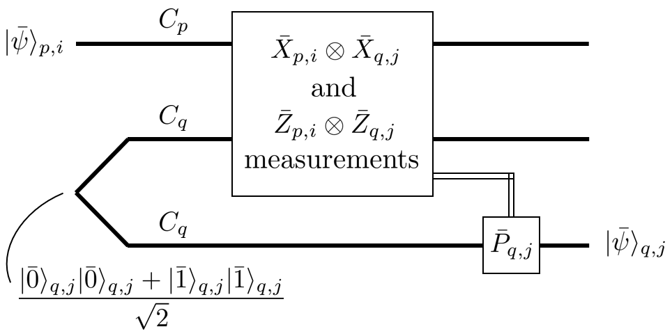
In conventional quantum teleportation, an EPR state and Bell measurement are required. Here we will examine a process to fault-tolerantly perform quantum teleportation of logical data between two code blocks. The scheme for logical qubit teleportation is shown in Fig. 5(a). Suppose that we would like to teleport the logical qubit of to the logical qubit of , first an EPR state prepared on is required. The logical qubit teleportation can be done by performing a Bell measurement with respect to and between and the first block of . The teleported logical qubit can be obtained in the second block of by operating an appropriate logical Pauli operator depending on the Bell measurement result. Note that the Bell measurement can be done fault-tolerantly using the measurement protocol in Section V, and logical Pauli operators are transversal (therefore, fault tolerant). Thus, fault-tolerant teleportation between two code blocks can be achieved.
Now let us consider fault-tolerant computation on cyclic CSS codes. It is known that for any error correcting code, by the Eastin-Knill theorem [28], at least one logical gate in a universal gate set cannot be implemented transversely. For such gates, other fault-tolerant techniques must be performed, which can require a significant amount of resources. Fortunately, fault-tolerant implementations of logical Clifford gates on distance-3 cyclic CSS codes can be achieved via quantum gate teleportation (see [29] for the details of quantum gate teleportation). For example, suppose that we would like to perform a logical Hadamard gate on the code . This can be achieved by preparing a codeword which is an eigenstate of and on , performing logical qubit teleportation, and operating a logical Pauli operator depending on the result from the Bell measurement in qubit teleportation as illustrated in Fig. 5(b). Also, logical and logical CNOT gates on any logical qubits can be performed in a similar way. The Clifford group can be generated by [30, 31]. Thus, our scheme is applicable to any Clifford operation. It is known that universal quantum computation can be achieved by Clifford gates and any other gate not in the Clifford group [32]. However, performing logical non-Clifford gates will require different techniques such as the ones presented in [19].

VII Examples of cyclic CSS codes
In this section, some examples of cyclic CSS codes satisfying Theorem 2 are given. A first example is the quantum Hamming code. This code is constructed from a classical [7,4,3] Hamming code (with ). A check polynomial of the [7,4,3] Hamming code in cyclic form is
| (23) |
In fact, any classical Hamming code can be made cyclic [21]. Thus, any CSS code constructed from a classical Hamming code with satisfies Theorem 2, and can be used in the flag-FTEC protocol and the flag-FT measurement protocol described in this work.
Another example of cyclic CSS codes satisfying Theorem 2 is the code constructed from a classical [30,22,3] cyclic code with a check polynomial
| (24) |
The [30,22,3] code and other classical codes satisfying are given in Table 1 of [27]. (A method of finding the check polynomial of a classical cyclic code is discussed in [21].) One possible choice of logical operators for the code is given in Table 1. The advantages of the code are that its encoding rate is high (), and the logical operators of the first ten logical qubits have a simple form, which make them easily accessible.
VIII Discussion and conclusion
In this work we used the symmetries of CSS codes constructed from classical cyclic codes to prove that errors written in consecutive form (as in Definition 7) can be distinguished. From these properties, we can obtain a 1-flag circuit along with a flag-FTEC protocol which satisfies the fault-tolerance criteria of Definition 2 when there is at most one fault. The 1-flag circuit requires only four ancilla qubits. This number does not grow as the block length gets larger, making our protocol advantageous in the implementation where resources are limited. We note that not all cyclic CSS codes are Hamming codes and therefore the methods in [12] (which apply to perfect codes) cannot be directly applied, thus providing further motivation for our work.
In general, cyclic CSS codes do not satisfy the sufficient condition required for flag fault-tolerance presented in [15] (one example is the family of Hamming codes which can be made cyclic). Nevertheless, using the techniques presented in this paper, a flag-FTEC protocol can still be achieved.
Furthermore, we have shown how logical Pauli operators of cyclic CSS codes can be fault-tolerantly measured using the flag techniques discussed in Section V. The flag-FT operator measurement protocol satisfies the fault-tolerance criteria of Definition 10 when there is at most one fault. We then showed in Section VI how one can fault-tolerantly perform quantum gate teleportation to implement logical Clifford operators on any given logical qubit for codes which encode multiple logical qubits. Examples of cyclic CSS codes with large encoding rates are provided in Section VII.
Note that for all CSS codes, the stabilizer generators being measured are of the form or up to qubit permutations. Thus data qubit errors arising from faulty CNOT gates will be expressed in consecutive form. The errors of this form are distinguishable iff the sub-matrices of the and stabilizers satisfy Lemma 1. In our work, we use the symmetry of the cyclic codes to simplify Lemma 1 into Lemma 3. We believe that Lemma 1 can be simplified by using symmetries found in other families of quantum codes. With appropriate -flag circuits and operations depending on the flag measurement outcome, this may lead to new flag fault-tolerant protocols.
Another interesting avenue is finding non-cyclic quantum codes for which a version of Theorem 2 can be applied. We note that for such codes, the same 1-flag circuit as in Fig. 3 along with the flag-FTEC protocol of Section IV and the flag-FT measurement protocol of Section V can be used. The reason is that the key property used by these schemes is based on the distinguishability of consecutive errors.
Note that there are quantum cyclic codes which are not CSS codes for which flag fault-tolerant schemes are still possible. For instance, a flag-FTEC protocol for the code was devised in [12]. We believe that it could be interesting to generalize the ideas presented in this work to non-CSS cyclic quantum codes. However, we leave this problem for future work.
The flag fault-tolerant protocols for cyclic CSS codes presented in this work are based on the assumption that the qubit measurement and state preparation must be fast since we reuse some flag qubits in the protocols (as we can see in Fig. 3). If we do not reuse flag qubits, however, the number of required ancillas will be for an operator being measured of the form instead of .
One important feature of flag fault-tolerant protocols is that the number of required ancillas is very small compared to other fault-tolerant schemes. We believe that if fewer ancillas are required, the accuracy threshold will increase since the number of locations will decrease in total. However, we should point out that subsequent syndrome measurements are also required in a flag fault-tolerant protocol and may increase the total number of locations in the protocol. The answer of whether the accuracy threshold for a flag fault-tolerant protocol is greater or smaller compared to other fault-tolerant schemes is still unknown.
Lastly, we point out that cyclic CSS codes which satisfy the condition in Theorem 2 are not limited to distance-3 codes. Therefore, interesting future work would be to use the methods of [15] to obtain flag fault-tolerant schemes for higher-distance codes. In particular, the main challenge stems from finding -flag circuits as in Fig. 3 for .
IX Acknowledgements
T.T. acknowledges the support of The Queen Sirikit Scholarship under The Royal Patronage of Her Majesty Queen Sirikit of Thailand. C.C. acknowledges the support of NSERC through the PGS D scholarship. D.L. is supported by an NSERC Discovery grant and a CIFAR research grant via the Quantum Information Science program.
References
- [1] P. W. Shor, “Fault-tolerant quantum computation,” Proceedings., 37th Annual Symposium on Foundations of Computer Science, pp. 56–65, 1996.
- [2] D. Aharonov and M. Ben-Or, “Fault-tolerant quantum computation with constant error,” in Proceedings of the twenty-ninth annual ACM symposium on Theory of computing, pp. 176–188, ACM, 1997.
- [3] J. Preskill, “Reliable quantum computers,” Proceedings of the Royal Society of London. Series A: Mathematical, Physical and Engineering Sciences, vol. 454, no. 1969, pp. 385–410, 1998.
- [4] E. Knill, R. Laflamme, and W. H. Zurek, “Threshold accuracy for quantum computation,” arXiv: quant-ph/9610011, 1996.
- [5] E. Dennis, A. Kitaev, A. Landhal, and J. Preskill, “Topological quantum memory,” Journal of Mathematical Physics, vol. 43, pp. 4452–4505, 2002.
- [6] A. G. Fowler, M. Mariantoni, J. M. Martinis, and A. N. Cleland, “Surface codes: Towards practical large-scale quantum computation,” Phys. Rev. A, vol. 86, p. 032324, Sep 2012.
- [7] Y. Tomita and K. M. Svore, “Low-distance surface codes under realistic quantum noise,” Phys. Rev. A, vol. 90, p. 062320, Dec 2014.
- [8] A. G. Fowler, A. C. Whiteside, A. L. McInnes, and A. Rabbani, “Topological code autotune,” Phys. Rev. X, vol. 2, p. 041003, Oct 2012.
- [9] A. Paetznick and B. W. Reichardt, “Fault-tolerant ancilla preparation and noise threshold lower boudds for the 23-qubit golay code,” Quantum Info. Comput., vol. 12, pp. 1034–1080, Nov. 2012.
- [10] C. Chamberland, T. Jochym-O’Connor, and R. Laflamme, “Overhead analysis of universal concatenated quantum codes,” Phys. Rev. A, vol. 95, p. 022313, Feb 2017.
- [11] R. Takagi, T. J. Yoder, and I. L. Chuang, “Error rates and resource overheads of encoded three-qubit gates,” Phys. Rev. A, vol. 96, p. 042302, Oct 2017.
- [12] R. Chao and B. W. Reichardt, “Quantum error correction with only two extra qubits,” Phys. Rev. Lett., vol. 121, p. 050502, Aug 2018.
- [13] R. Chao and B. W. Reichardt, “Fault-tolerant quantum computation with few qubits,” npj Quantum Information, vol. 4, no. 1, p. 42, 2018.
- [14] B. W. Reichardt, “Fault-tolerant quantum error correction for Steane’s seven-qubit color code with few or no extra qubits,” arXiv e-prints, p. arXiv:1804.06995, Apr 2018.
- [15] C. Chamberland and M. E. Beverland, “Flag fault-tolerant error correction with arbitrary distance codes,” Quantum, vol. 2, p. 53, Feb. 2018.
- [16] A. A. Kovalev and L. P. Pryadko, “Fault tolerance of quantum low-density parity check codes with sublinear distance scaling,” Phys. Rev. A, vol. 87, p. 020304, Feb 2013.
- [17] D. Gottesman, “Fault-tolerant quantum computation with constant overhead,” Quantum Info. Comput., vol. 14, pp. 1338–1372, Nov. 2014.
- [18] J. P. Tillich and G. Zémor, “Quantum ldpc codes with positive rate and minimum distance proportional to the square root of the blocklength,” IEEE Transactions on Information Theory, vol. 60, pp. 1193–1202, Feb 2014.
- [19] C. Chamberland and A. W. Cross, “Fault-tolerant magic state preparation with flag qubits,” Quantum, vol. 3, p. 143, May 2019.
- [20] Y. Shi, C. Chamberland, and A. W. Cross, “Fault-tolerant preparation of approximate GKP states,” arXiv e-prints, p. arXiv:1905.00903, May 2019.
- [21] F. J. MacWilliams and N. J. A. Sloane, The theory of error-correcting codes. North-Holland, New York, 1977.
- [22] D. Gottesman, “Class of quantum error-correcting codes saturating the quantum Hamming bound,” Phys. Rev. A, vol. 54, pp. 1862–1868, 1996.
- [23] D. Gottesman, Stabilizer Codes and Quantum Error Correction. PhD thesis, California Institute of Technology, 1997.
- [24] A. R. Calderbank and P. W. Shor, “Good quantum error-correcting codes exist,” Phys. Rev. A, vol. 54, pp. 1098–1105, Aug 1996.
- [25] A. W. Steane, “Multiple-Particle Interference and Quantum Error Correction,” Proc. Roy. Soc. Lond., vol. 452, pp. 2551–2577, 1996.
- [26] P. Aliferis, D. Gottesman, and J. Preskill, “Quantum accuracy threshold for concatenated distance-3 codes,” Quantum Info. Comput., vol. 6, no. 2, pp. 97–165, 2006.
- [27] R. Li and X. Li, “Quantum codes constructed from binary cyclic codes,” International Journal of Quantum Information, vol. 02, no. 02, pp. 265–272, 2004.
- [28] B. Eastin and E. Knill, “Restrictions on transversal encoded quantum gate sets,” Phys. Rev. Lett., vol. 102, p. 110502, 2009.
- [29] D. Gottesman and I. L. Chuang, “Demonstrating the viability of universal quantum computation using teleportation and single-qubit operations,” Nature, vol. 402, no. 6760, p. 390, 1999.
- [30] A. R. Calderbank, E. M. Rains, P. W. Shor, and N. J. Sloane, “Quantum error correction and orthogonal geometry,” Physical Review Letters, vol. 78, no. 3, p. 405, 1997.
- [31] D. Gottesman, “Theory of fault-tolerant quantum computation,” Phys. Rev. A, vol. 57, no. 1, p. 127, 1998.
- [32] G. Nebe, E. M. Rains, and N. J. Sloane, “The invariants of the clifford groups,” Designs, Codes and Cryptography, vol. 24, no. 1, pp. 99–122, 2001.
Appendix A Proof of the lemmas
Proof of Lemma 1: We will prove that is distinguishable by iff for all such that , there exists such that . Consider errors and where . Let be error syndromes corresponding to errors and , respectively. By Definition 5, and are distinguishable by iff , i.e., there exists such that (here corresponds to the component of and ). From the parity check matrix , the component of and is given by
| (25) | ||||
| (26) |
From Eqs. 25 and 26, we have that
| (27) |
Thus, is distinguishable by iff for all such that , there exists such that
| (28) |
The proof of the statement for is similar.
Now we will proof that is distinguishable by iff both and are distinguishable by . Let and , where . Observe that any element of is of the form where and . The syndrome of is . If is distinguishable by , i.e., for all choices of such that , then we have that any pair of and and any pair of and are distinguishable. Conversely, if any pair of and and any pair of and are distinguishable, then any pair of and will have different syndromes. This implies Statement 3.
Proof of Lemma 2: Suppose that the stabilizer group of can be generated by . Since is a CSS code, we will first assume that the generators ’s are either -type or -type, denoted as or . Let and be and stabilizer matrices of the code in symplectic representation, and let and be the classical codes generated by and , respectively. Observe that any element of in symplectic representation is of the form where and . For any choice of , let (or ) be the parity check matrix corresponding to ’s (or ’s). We find that the code generated by (or generated by ) differs from (or ) by an -step left cyclic permutation. However, since and are cyclic codes, we have that and . Therefore, and generate the same stabilizer group for any .
In general, some generators of the stabilizer group of might be neither -type nor -type. The following transformations of the generators preserve the stabilizer group, and the last set of generators is the cyclic shifts of the original: (1) Transform the given generators to either -type or -type. This corresponds to appropriate reversible row operations on the binary symplectic representation of to obtain the block diagonal form,
| (29) |
(2) Cyclic shifts of these new generators also generate the same stabilizer group. (3) Reversing the transformation in step (1) (now applied to the generators after step (2)) preserves the stabilizer group. The resulting generators are cyclic shifts of the original.
Proof of Lemma 3: First we will prove that is distinguishable by iff for all , there exists such that . Applying Lemma 1, we would like to prove that for all such that , there exists such that iff for all , there exist such that .
By choosing and , the proof is trivial.
Assume by contradiction that there exists a pair of with such that for all ; i.e., there exists a pair of errors and which cannot be distinguished by any generator of . Let be generated by . By Lemma 2, we can construct a new generator set of where for all . Let the -part of be . Note that and . The assumption implies that and cannot be distinguished by any as well. This gives
| (30) |
or equivalently,
| (31) |
Let . Therefore, there exists such that for all .
The proof of statement for is similar to the proof of statement for , while the proof of statement for is similar to the proof of Statement 3 in Lemma 1.
| Type of faults | Correction procedure |
|---|---|
| No fault | 1 |
| Qubit or measurement fault on | 1 or 2 |
| Qubit or measurement fault on | 1 or 4(a) |
| Qubit or measurement fault on | 1 or 3 |
| Red CNOT fault with or error on the target qubit | 2 |
| Red CNOT fault with or error on the target qubit | 4(b) |
| Blue or green CNOT fault with or error on the target qubit | 1 or 2 or 3 |
| Blue or green CNOT fault with or error on the target qubit | 4(b) or 4(c) |
| Orange CNOT fault with or error on the target qubit | 1 or 2 or 4(a) |
| Orange CNOT fault with or error on the target qubit | 2 or 4(a) |
| Type of faults | Correction procedure |
|---|---|
| —— No fault during operator measurement —— | |
| No input error, no fault during syndrome measurement | 1(a) |
| No input error, one fault during syndrome measurement | 1(b) or 1(c) |
| weight-1 input error, no fault syndrome measurement | 1(c) |
| —— One fault during operator measurement —— | |
| Qubit or measurement fault on | 2 |
| Qubit or measurement fault on | 4(a) |
| Qubit or measurement fault on | 3 |
| Red CNOT fault with or error on the target qubit | 2 |
| Red CNOT fault with or error on the target qubit | 4(b) |
| Blue or green CNOT fault with or error on the target qubit | 1(a) or 2 or 3 |
| Blue or green CNOT fault with or error on the target qubit | 4(b) or 4(c) |
| Orange CNOT fault with or error on the target qubit | 1(a) or 2 or 4(a) |
| Orange CNOT fault with or error on the target qubit | 2 or 4(a) |
We already proved statements for , , and . We will generalize the statements to , , and for any . Let by a cyclic CSS code generated by . Observe that by qubit reordering, is distinguishable by iff is distinguishable by . Since and are the same code by Lemma 2, we have that is distinguishable by for any iff is distinguishable by . The proof is also applied to and .
Appendix B Lists of possible faults during FTEC and FT operator measurement protocols
The lists of possible faults during the flag-FTEC protocol (see Section IV) and the flag-FT operator measurement protocol (see Section V) are given in Tables 2 and 3, respectively. The corresponding correction procedure for each type of faults refers to the step of either flag-FTEC protocol or flag-FT operator measurement protocol. Here we assume that in the flag-FTEC protocol and in the flag-FT operator measurement protocol, where is the number of input errors and is the number of faults.