Correcting the Mistaken Identification of Nonequilibrium Microscopic Work

In this work, we are mainly interested in an interacting system $\Sigma$ in the presence of a medium $\widetilde{\Sigma}$ as shown in Fig. 1; the latter will be taken to be a collection of two parts: a work source $\widetilde{\Sigma}_{\text{w}}$ and a heat source $\widetilde{\Sigma}_{\text{h}}$, both of which can interact with the system $\Sigma$ directly but not with each other. We will continue to use $\widetilde{\Sigma}$ to refer to both of them together. The collection $\Sigma_{0}=\Sigma\cup\widetilde{\Sigma}$ forms an isolated system, which we assume to be stationary, with all of of its observables such as its energy $E_{0}$, its volume $V_{0}$, its number of particles (we assume a single species) $N_{0}$ constant in time, even if there may be internal changes going on when its parts are out of equilibrium. These internal changes require some internal variables for their description [1, 2, 3]. In the following, we will assume $\widetilde{\Sigma}$ to be always in equilibrium (which requires it to be extremely large compared to $\Sigma$) so that any irreversibility going on within $\Sigma_{0}$ is ascribed to $\Sigma$ alone, and is caused by processes such as dissipation due to viscosity, internal inhomogeneities, etc. that are internal to the system. Moreover, we assume additivity of volume, a weak interaction between, and quasi-independence of, $\Sigma$ and $\widetilde{\Sigma}$; the last two conditions ensure that the energies and entropies are additive [4, 5, 8, 7, 6] but also impose some restriction on the size of $\Sigma$ in that it cannot be too small. In particular, the size should be at least as big as the correlation length for quasi-independence as discussed earlier [5, 8, 7]. In this work, we will assume that all required conditions necessary for the above-mentioned additivity are met.

All quantities pertaining to $\Sigma$ carry no suffix; those for $\widetilde{\Sigma}$ carry a tilde, while those of $\Sigma_{0}$ carry a suffix $0$. As $\widetilde{\Sigma}$ is always in equilibrium, all its fields have the same value as for $\Sigma_{0}$ so that its temperature, pressure, etc. are shown as $T_{0},P_{0}$, etc. as seen in Fig. 1. To simplify our discussion, we are going to mostly restrict our discussion to two parameters in the Hamiltonian; however, later in Secs. IX-X, we will consider a general set $\mathbf{W}$ of work parameters. In equilibrium (EQ), the state of $\Sigma$ is described by two observables $E$ and $V$ of which $V$ appears as a parameter in its Hamiltonian $\mathcal{H}(\mathbf{z},V)$; here, $\mathbf{z}$ is the collection of coordinates and momenta of the $N$ particles. Throughout this work, $N$ is kept fixed so we will not exhibit it unless necessary. We can manipulate $V$ from the outside through $\widetilde{\Sigma}_{\text{w}}$, which exerts an external ”force” such as the pressure to do some ”work.” For this work, $V$ is a symbolic representation of an externally controlled parameter, which is commonly denoted by $\lambda$ in the current literature and whose nature is determined by the experimental setup. Thus, $V$ here should be considered a parameter in a wider sense than just the volume and $P$ its conjugate force; see Fig. (2).

The EQ entropy is a state function $S(E,V)$. Away from EQ, we also need an additional set of independent extensive internal variables to specify the state [1, 2, 3]; we take a single variable $\xi$ for our study to simplify the presentation [9]. In this case, $V$ and $\xi$ appear as parameters in the Hamiltonian $\mathcal{H}(\mathbf{z},V,\xi)$. However, the discussion can be readily extended to many internal variables. The force conjugate to $\xi$ is known as the affinity and conventionally denoted by $A$ [1, 2, 3]. A NEQ state for which its entropy is a state function $S(E,V,\xi)$ is said to be an internal equilibrium (IEQ) state [4, 5]. We will only consider IEQ states in this work for simplicity. It is well known that the energy $E=\mathcal{H}_{V,\xi}$ does not change at fixed $V$ and $\xi$ as $\mathbf{z}$ evolves in accordance with Hamilton’s equations of motion. Therefore, $\mathbf{z}$ plays no role in the performance of work so we will usually not exhibit it unless clarity is needed.

Focus on the Hamiltonian $\mathcal{H}(V,\xi)$ provides us with the advantage of obtaining a microscopic description of NEQ thermodynamics, where a central role is played by the microscopic work-Hamiltonian relation at the level of microstates $\left\{\mathfrak{m}_{k}\right\}$ of a NEQ system $\Sigma$. The work relation is a key ingredient in developing a microscopic NEQ statistical thermodynamics, where the emphasis is in the application of the first law in diverse branches including but not limited to nonequilibrium work theorems, [10, 11, 12, 13] stochastic thermodynamics, [14, 15] and quantum thermodynamics, [16, 17] to name a few. Once microscopic work is identified, microscopic heat can also be identified by invoking the first law. This makes identifying work of primary importance in NEQ thermodynamics. Unfortunately, this endeavor has given rise to a controversy about the actual meaning of NEQ work, which apparently is far from settled [18, 19, 20, 21, 22, 23, 24, 25, 26, 27, 28, 13, 10].

The above controversy is distinct from the confusion about the meaning of work and heat in classical nonequilibrium thermodynamics [29, 30] involving a system-intrinsic (SI) or medium-intrinsic (MI) description, the latter only recently having been clarified [31, 32, 4, 5, 6, 7, 8]; see Sec. III for more details and clarification.

The SI-work $dW$ is the work done by the system and the MI-work $d\widetilde{W}$ is the work done by the medium. At the level of microstates, one is faced with the fact that both of these works $dW_{k}$ and $d\widetilde{W}_{k}$ cannot be related to the change $dE_{k}$ in the microstate energy of $\mathfrak{m}_{k}$. Indeed, as pointed out recently [33], the identification of microscopic work has proven erroneous in that the external work $d\widetilde{W}_{k}$, an MI quantity for $\mathfrak{m}_{k}$, is identified with the SI energy change $dE_{k}$ for $\mathfrak{m}_{k}$, whereas in a NEQ state, the thermodynamics of the medium and the system are very different. As pointed above, it is $\Sigma$ that experiences dissipation [29, 30, 34], which is partly responsible for the irreversible entropy generation $d_{\text{i}}S$ in the system. This dissipation is not captured by $d\widetilde{W}_{k}$ in its current formulation as we will see in this work. This is related to a surprising fact hitherto unappreciated that at the microscopic level, $d\widetilde{W}_{k}$ and $dE_{k}$ always differ in a thermodynamic system, even when dealing with a reversible process as shown by a thermodynamic example in Sec. VII.2. In fact, they differ even for a purely mechanical system as shown by the mechanical example in Sec. VII.1.

Jarzynski Equality: As we will show here (this has been briefly reported earlier [33]), not recognizing this subtle fact has given rise to the ”mistaken identity”

$$d\widetilde{W}_{k}\overset{?}{=}dE_{k},$$

(1)

between an MI-work and SI-energy change in the current literature; see for example Jarzynski [11] who exploits the mistaken identity to prove by now the famous Jarzynski equality (JE) discussed below in Sec. III.3.

Following Prigogine [2], see also Fig. (1) and Sec. II for clarification, we partition

$$dE_{k}=d_{\text{e}}E_{k}+d_{\text{i}}E_{k},$$

(2)

in which $d_{\text{e}}E_{k}\equiv d\widetilde{W}_{k}$ represents the change caused by the exchange with $\widetilde{\Sigma}$ through external work and $d_{\text{i}}E_{k}$ represents the change caused by internal processes going on within $\Sigma$. As the work $dW_{k}$ is the work done by $\mathfrak{m}_{k}$ at the expense of its energy loss, we have $dW_{k}=-dE_{k}$ as we will establish here. We will show by examples and arguments that $d_{\text{i}}E_{k}\neq 0$ is ubiquitous not only in purely mechanical systems but also in a reversible process and is necessary for dissipation. The main thesis of this work to be established here is the following

The same conclusion also applies to the accumulation $\Delta_{\text{i}}E_{k}\neq 0$ along a trajectory, which is the path $\gamma$ taken by the $k$th microstate $\mathfrak{m}_{k}$ during a NEQ process $\mathcal{P}_{0}$ over a time interval $\left(0,\tau\right)$. The energy changes $dE_{k},d_{\text{e}}E_{k}$ and $d_{\text{i}}E_{k}$ occur during a segment of $\mathcal{P}_{0}$ between $t$ and $t+dt$, while $\Delta E_{k},\Delta_{\text{e}}E_{k}$ and $\Delta_{\text{i}}E_{k}$ are cumulative changes over the entire trajectory $\gamma$; see Sec.V for more details.

Quantum and Stochastic Thermodynamics: In a seminal paper laying down the foundation of quantum thermodynamics, Alicki [17, cf. Eq. (2.4) there] identifies the average work $d\widetilde{W}$, the average of $d\widetilde{W}_{k}$, done by external forces with the average of $dE_{k}$ in accordance with Eq. (1). In a paper of similar importance for stochastic thermodynamics, Sekimoto [14, cf. Eqs. (2.7)-(2.9) there] also identifies the change $dE_{k}$ in the energy $E_{k}$ by work variables with the work $d\widetilde{W}_{k}$ done by the external system.

What is Accomplished: The recent report [33] was very compact. This work is designed to elaborate on what was reported, to provide the missing details and more. Throughout the work, we include an internal varaiable as a work variable. The main emphasis here will be to demonstrate the ubiquitous nature of $d_{\text{i}}E_{k}$, whose existence has not been previously appreciated. Not recognizing its existence has resulted in the above mistaken identification. It is the force imbalance between the internal and external forces that generates $d_{\text{i}}E_{k}$ and is very common in almost processes, even a reversible one as we will demonstrate. This is the most important outcome of the our approach, which emphasizes the importance of SI-quantities (such as $dE_{k}=-dW_{k}$) that are very different from the MI-quantities (such as $d_{\text{e}}E_{k}=d\widetilde{W}_{k}$) in any process, even a reversible one. The use of generalized work as isentropic change $dW=-dE_{S}$ allows us to calculate microscopic work $dW_{k}$, which changes $dE_{k\text{ }}$but not $p_{k}$. On the other hand, the generalized heat $dQ_{k}$ does not change $dE_{k}$ but changes $p_{k}$. This proves to be a great simplification and allows us to treat $dW_{k}$ and $dQ_{k}$ as purely a mechanical and a stochastic concept, respectively. In addition, as $\mathfrak{m}_{k}$ uniquely determines $E_{k}$ for a fixed work set $\mathbf{W}$, we find that $dE_{k}$ is uniquely determined by $d\mathbf{W}$ and not by the nature of the work process. This provides a simplification in evaluating the cumulative change $\Delta W_{k}$ and allows us to prove a new work theorem, both for the exclusive and the inclusive Hamiltonian. This work theorem is very general and we apply it successfully to the free expansion.

The layout of the paper is the following. In the next section, we introduce the extension of Prigogine’s notation as it may be unfamiliar to many readers. In Sec. III, three important concepts of NEQ quantities that will play a central role in this work: the concepts of SI- and MI-quantities, and that of microwork. In Sec. IV, we give two alternate versions of the first law using the MI- and SI-quantities, and introduce thermodynamic forces and their role in dissipation that does not seem to have been appreciated in the field. A new concept of force imbalance is also introduced that plays an important role in microscopic thermodynamics but has been hitherto overlooked. It is one of the central new quantities that is ubiquitous and needs to be incorporated in any process, EQ or NEQ. In Sec. V, we introduce a new approach to investigate NEQ thermodynamics at the microscopic level by using microstates. Here, we introduce a different way of looking at work and heat, which we call generalized work and generalized heat, that has only recently been developed but proves very useful for a microscopic understanding of statistical thermodynamics. The generalized work is isentropic and the generalized heat satisfies the Clausius equality $dQ=TdS$ even for an irreversible process. This makes generalized work a purely mechanical quantity. The stochasicity arises from heat but not from work. This results in a clear division between work and heat, making them independent quantities as we explain here. In the next section, we introduce exclusive and inclusive Hamiltonians. It is the latter Hamiltonian that is used by Jarzynski, but we find basically no formal difference between the two. In Sec. VII, we consider two different models, a mechanical and a thermodynamic, to explain various different kinds of NEQ work and heat. In Sec. VIII, we show how internal variables emerge in a system’s Hamiltonian. We particularly pay attention to the relative velocity that induces a force that is dissipative, i.e., frictional and contributes to the dissipative work. In Sec. IX, we finally develop our theoretical framework for NEQ statistical thermodynamics and introduce statistical formulation of various quantities. In Sec. X, we propose a new work theorem both for an exclusive and an inclusive Hamiltonian, which differs from the Jarzynski formulation. The latter is well known for its failure for free expansion. Therefore, we apply the new theorem to free expansion and show that it holds in Sec. XI. Indeed, we argue that the new theorem works for any arbitrary process and not just the free expansion. In the last section, we give a brief summary of our results.

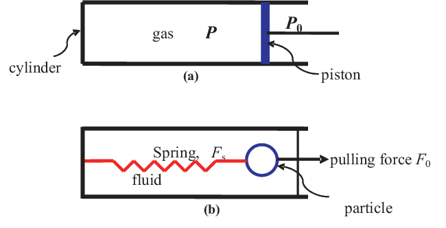
In a NEQ state, the thermodynamics of the medium and the system are very different. As pointed above, it is $\Sigma$ that experiences dissipation [29, 30, 34], which is partly responsible for the irreversible entropy generation $d_{\text{i}}S$ in the system as we will see in Eq. (35). To clarify the difference between the SI-description and the MI-description, we consider the pressure-volume work and the work done by some internal variable $\xi$ as an example; see the gas confined in a cylinder with one end closed and a movable piston on the other end in Fig. 2(a). The internal variable may describe the nonuniformity of the gas in an irreversible process. It should be recalled that a system in EQ must be uniform [5, 35] so any nonuniformity will result in a NEQ state. The work in the two descriptions is the

$$\text{SI-work }dW=PdV+Ad\xi$$

(12)

done by $\Sigma$ (SI) or the

$$\text{MI-work}\emph{\ }d\widetilde{W}=-P_{0}dV$$

(13)

done by $\widetilde{\Sigma}$ (MI) in terms of the instantaneous pressure $P$ of $\Sigma$ or $P_{0}~$of $\widetilde{\Sigma}$, and their volume change $dV$ or $-dV$, respectively, where we have used the additivity of the volume $V_{0}=V+\widetilde{V}$ and the fact that $d\widetilde{V}=-dV$ to ensure a constant $V_{0}$. Notice that $d\widetilde{W}$ does not contain any contribution from the internal variable since $A_{0}=0$ [1, 2]. It represents the MI-work done on the system by $\widetilde{\Sigma}$ and its negative denotes the exchange work between $\widetilde{\Sigma}$ and $\Sigma$ as the MI-work done by $\Sigma$ against $\widetilde{\Sigma}$; we denote it by

$$d_{\text{e}}W=-d\widetilde{W}=P_{0}dV.$$

Let $d\widetilde{Q}$ denote the heat added to the medium $\widetilde{\Sigma}$, here by the system. Then, $d_{\text{e}}Q=-d\widetilde{Q}$ is the heat transferred (exchanged) to $\Sigma$ by $\widetilde{\Sigma}$ and $d_{\text{e}}W=-d\widetilde{W}$ is the work transferred (exchanged) by $\Sigma$ to $\widetilde{\Sigma}$. Both $d_{\text{e}}Q$ and $d_{\text{e}}W$ refer to energy flows across the boundary between $\Sigma$ and $\widetilde{\Sigma}$ (see the exchange $d_{\text{e}}X$ in Fig. 1), and are determined by the process of transfer that depends on the combined properties of $\Sigma$ and $\widetilde{\Sigma}$. They are customarily used to express the first law for $\Sigma$

$$dE=d_{\text{e}}Q-d_{\text{e}}W$$

(14)

Our sign convention is that $d_{\text{e}}Q$ is positive when it is added to $\Sigma$, and $d_{\text{e}}W$ is positive when it is transferred to $\widetilde{\Sigma}$. Once, work has been identified, the use of the first law allows us to uniquely determine the heat.

The above macroscopic concepts of work represent thermodynamic averages (this will become more clear later) [35, 30, 34, 36]. This allows us to identify the microscopic analogs $dW_{k}$ and $d\widetilde{W}_{k}$ of $dW$ and $d\widetilde{W}$, respectively, at the level of $k$th microstates $\mathfrak{m}_{k}$. The thermodynamic average connection, see also Sec. V, is the following:

$$dW=\left\langle dW\right\rangle\doteq{\textstyle\sum\nolimits_{k}}p_{k}dW_{k},d\widetilde{W}=\left\langle d\widetilde{W}\right\rangle\doteq{\textstyle\sum\nolimits_{k}}p_{k}d\widetilde{W}_{k},$$

(15)

which also introduces thermodynamic averaging $\left\langle\cdot\right\rangle$ with respect to the instantaneous microstate probabilities $\left\{p_{k}\right\}$. For the energy change $dE_{k}$, we have its average given by

$$dE_{S}=\left\langle dE\right\rangle\doteq{\textstyle\sum\nolimits_{k}}p_{k}dE_{k};$$

(16)

the reason for the special symbol becomes once we recall the definition of entropy $S$:

$$S=-\left\langle\ln p\right\rangle\doteq-{\textstyle\sum\nolimits_{k}}p_{k}\ln p_{k}.$$

(17)

As the above three averages are at fixed $p_{k}$’s, they are evaluated at fixed entropy. This is shown by the suffix $S$ in $dE_{S}$. This quantity will turn out to have an important role in our theory.

We will refer to $dW_{k}$ in the following as microstate work or microwork in short (but not $d\widetilde{W}_{k}$). One can then determine the accumulated work $\Delta W_{k},\Delta\widetilde{W}_{k}$ and $\Delta E_{k}$ along some path $\gamma$ followed by the microstate in some process $\mathcal{P}_{0}$ by simply integrating $dW_{k}$ but without the probabilities:

$$\Delta W_{k}\doteq{\textstyle\int\nolimits_{\gamma}}dW_{k},\Delta\widetilde{W}_{k}\doteq{\textstyle\int\nolimits_{\gamma}}d\widetilde{W}_{k},\Delta E_{k}\doteq{\textstyle\int\nolimits_{\gamma}}dE_{k}.$$

(18)

We observe that $dW_{k},d\widetilde{W}_{k}$ and $dE_{k}$ are defined regardless of the probability $p_{k}$. Because of this, we wish to emphasize the following important point, which we present as a

This condition will prove useful when we consider free expansion of a classical gas in Sec. XI.

Traditional formulation of NEQ statistical mechanics and thermodynamics [35, 36] takes a mechanical approach in which $\Sigma$ follows its classical or quantum mechanical evolution dictated by its SI-Hamiltonian $\mathcal{H}(V,\xi)$ [9]; the interaction with $\widetilde{\Sigma}$ is usually treated as a very weak stochastic perturbation. However, investigating microwork (SI approach) is very convenient as $p_{k}$’s do not change. Unfortunately, this description has been overlooked by the current practitioners in the field who have consistently used a MI-description for work by using the external approach but then mistakenly confuse it with its SI-analog; see Eq. (1).

As $\Delta\widetilde{W}_{k}$ is not affected by the internal state ($P,A$, and $\left\{p_{k}\right\}$) of $\Sigma$, it is a choice candidate for studying work fluctuations and for the Jarzynski process. By setting the MI-works $d\widetilde{W}_{k},\Delta\widetilde{W}_{k}$ equal to the SI-changes $dE_{k},\Delta E_{k}$, respectively,

$$d\widetilde{W}_{k}=dE_{k},\Delta\widetilde{W}_{k}=\Delta E_{k},$$

(19)

[compare with Eq. (1)] Jarzynski developed the following famous nonequilibrium work relation, the JE, using a very clever averaging $\left\langle\cdot\right\rangle_{0}$

$$\left\langle e^{-\beta_{0}\Delta\widetilde{W^{\prime}}}\right\rangle_{0}\doteq{\textstyle\sum\nolimits_{k}}p_{k0}e^{-\beta_{0}\Delta\widetilde{W^{\prime}}_{k}}=e^{-\beta_{0}\Delta F^{\prime}}~$$

(20)

for a Jarzynski process (we use a prime now reserved for the inclusive approach discussed in Sec. VI). In Eq. (20), where an externally driven nonequilibrium process $\mathcal{P}_{0}$ between two equilibrium states, the initial state A${}_{\text{eq}}$ and the final state B${}_{\text{eq}}$, at the same inverse temperature $\beta_{0}$ is considered, $\left\langle\cdot\right\rangle_{0}$ refers to a special averaging with respect to the canonical probabilities of the initial state A${}_{\text{eq}}$:

$$p_{k0}^{\prime}\doteq e^{-\beta_{0}E_{k}^{\prime}}/Z_{\text{in}}^{\prime}(\beta_{0});$$

here, the suffix $0$ refers to the initial state A${}_{\text{eq}}$, $Z_{\text{in}}^{\prime}(\beta_{0})$ the initial equilibrium partition function for the system, $\Delta\widetilde{W^{\prime}}_{k}$ the cumulative work done on $\mathfrak{m}_{k}$ during $\mathcal{P}_{0}$, and $\Delta F^{\prime}$ the change in the free energy over $\mathcal{P}_{0}$ [37]. However, the average $\left\langle\cdot\right\rangle_{0}$ in Eq. (20) does not represent a thermodynamic average [compare with Eq. (53)] over $\mathcal{P}_{0}$ as recently pointed out [37]. The inverse temperature along $\mathcal{P}_{0}$ may not always exist or may be different than $\beta_{0}$ due to irreversibility [18, 38]. The process $\mathcal{P}_{0}$ consists of two stages: in the driving stage $\mathcal{P}$, external work is done ($\Delta\widetilde{W}_{k}^{\prime}\neq 0$), and the reequilibration stage $\overline{\mathcal{P}}\doteq\mathcal{P}_{0}\backslash\mathcal{P}$ ($\mathcal{P}_{0}=\mathcal{P\cup}\overline{\mathcal{P}}$) in which $\Sigma$ is in thermal contact with the heat bath $\widetilde{\Sigma}_{\text{h}}$ at $\beta_{0}$, during which no work is done ($\Delta\widetilde{W}_{k}^{\prime}\equiv 0$); $\widetilde{\Sigma}_{\text{h}}$ may or may not be present during $\mathcal{P}$. The equality is not obeyed for free expansion of a classical gas for which $\Delta\widetilde{W^{\prime}}_{k}\equiv 0$ but $\Delta F^{\prime}\neq 0$ as previously observed [20, 21, 22].

For the IEQ entropy $S(E,V,\xi)$, the Gibbs fundamental relation [36] is given by

$$dS=(dE+PdV+Ad\xi)/T,$$

(21)

where

$$1/T=\partial S/\partial E,P=T\partial S/\partial V,A=T\partial S/\partial\xi$$

are the inverse temperature, pressure and the affinity of the system that represent its fields. As $S$ is a SI-quantity, the above fields are also SI-quantities. In EQ, the affinity vanishes, which means that $S$ no longer depends on $\xi$. In other words, $\xi$ is no longer independent of $E$ and $V$ in EQ so we can write it as $\xi_{\text{eq}}\equiv\xi(E,V)$. Otherwise, $\xi$ is an independent variable in NEQ states. We can rewrite Eq. (21) as

$$dE=TdS-PdV-Ad\xi.$$

(22)

We see that the first term on the right side of the equation represents the change in the energy due to the entropy, while the last two terms represent the isentropic change $dE_{S}$ in the energy; see Eq. (16). These changes represent SI-changes in $E$ and play an important role in our approach. In particular, as $V$ and $\xi$ are work variables that we collectively denote by $\mathbf{W}$, we see from Eq. (12) that $\left.dE\right|_{S}$ is nothing but the SI-work $dW$. Thus,

$$TdS=dE-dE_{S}\equiv dE_{\mathbf{W}}\text{,}$$

(23)

where $dE_{\mathbf{W}}$ represents the change $dE$ at fixed $\mathbf{W}$. For brevity, we will call $dE_{\mathbf{W}}$ the isometric change in which all work variables are held fixed. Thus, we arrive at the following conclusion:

The conclusion allows us to express the first law in an alternative form using SI-quantities as we discuss below.

Using the exchange work $d_{\text{e}}W=-d\widetilde{W}=P_{0}dV$, the (MI) work done by $\Sigma$ against $\widetilde{\Sigma}$, and the work partition

$$dW=d_{\text{e}}W+d_{\text{i}}W,$$

(24)

we identify $d_{\text{i}}W$. We also introduce the exchange heat $d_{\text{e}}Q=-d\widetilde{Q}=T_{0}d_{\text{e}}S$ between $\widetilde{\Sigma}$ and $\Sigma$, which represents a MI-quantity. Defining

$$d_{\text{i}}Q\doteq d_{\text{i}}W$$

(25)

to emphasize the well-known fact that internal work can also be treated as internal heat, we introduce

$$dQ=d_{\text{e}}Q+d_{\text{i}}Q$$

(26)

so that the conventional MI-form of the first law in Eq. (14) can also be written in an SI-form

$$dE=dQ-dW.$$

(27)

From now on, we will refer to $dW$ and $dQ$ ($d_{\text{e}}W$ and $d_{\text{e}}Q$) as generalized work and generalized heat (exchange work and exchange heat), respectively, so that no confusion can arise.

If we compare this form with Eq. (22), we recognize that the last two terms there is $dW$ above. Hence, the first term $TdS$ there is nothing but $dQ$ introduced above. This provides us with an important consequence of our approach [31, 32, 4, 5, 6, 7, 8] in which

$$dQ=TdS;$$

(28)

compare with Eq. (23). In other words, $dQ$ is nothing but the isometric change $\left.dE\right|_{\mathbf{W}}$ in $E$: it is the change when no work is done ($dW=0$). The relation $dQ=TdS$ is very interesting in that it not only turns the well-known Clausius inequality $d_{\text{e}}Q=T_{0}d_{\text{e}}S\leq$ $T_{0}dS$ into an equality but also makes the generalized work $dW$ in Eq. (27) isentropic, whereas $d_{\text{e}}W=-d\widetilde{W}$ is not. This aspect of $dW$ will prove useful later. Moreover, Eq. (27) allows us to uniquely identify generalized heat and work; this work is always isentropic and this heat is always isometric. On the other hand, the MI-heat and the MI- work suffer from ambiguity; see, for example, Kestin [30]. We summaries these important observations here as

It is important to draw attention to the following important fact. We first recognize that the first law in Eq. (14) really refers to the change in the energy caused by exchange quantities. Therefore, $dE$ on the left truly represents $d_{\text{e}}E$; see Eq. (7). Accordingly, we write Eq. (14) as

$$d_{\text{e}}E=d_{\text{e}}Q-d_{\text{e}}W.$$

(29)

Subtracting this equation from Eq. (27), we obtain the identity

$$d_{\text{i}}E=d_{\text{i}}Q-d_{\text{i}}W\equiv 0,$$

(30)

where we have used Eq. (8). The above equation is nothing but the identity in Eq. (25). However, the analysis also demonstrates the important fact that the first law can be applied either to the exchange process or to the interior process. In the last formulation, it is also applicable to an isolated system.

The analog of $d_{\text{i}}W$ between two nearby equilibrium states is well known in classical thermodynamics and is usually called the dissipated work; see for example, p. 12 in Woods [34]. The dissipated work $(P-P_{0})dV$ is the difference between the generalized work $dW=PdV$ and the reversible work $dW_{\text{rev}}=P_{0}dV$ done by $\Sigma$ between the same two equilibrium states and is always nonnegative in accordance with Theorem 17 that will be proved later in its general form (which refers to $d_{\text{i}}W$ between any two nearby arbitrary states that need not necessarily be equilibrium states). If they are not, then the procedure described by Wood to determine dissipated work cannot work as there is no reversible path connecting two nonequilibrium states. This makes our approach for introducing $d_{\text{i}}W=dW-d_{\text{e}}W$ much more general.

We rewrite $dE$ in Eq. (27) as

$$dW=TdS-dE=-dF+(T-T_{0})dS,$$

where

$$F=E-T_{0}S$$

(31)

is the Helmholtz free energy; note the presence of $T_{0}$ and not $T$ in $F$. As $(T-T_{0})dS\leq 0$ established later, see Eq. (71), we conclude

$$dW\leq-dF,$$

(32)

as a consequence of the second law. It is also easy to see from this that

$$d\widetilde{W}\geq dF+d_{\text{i}}W\geq dF,$$

(33)

where we have used the fact that $d_{\text{i}}W\geq 0$, which is again a consequence of the second law as shown in Theorem 17. Similar inequalities also hold in the inclusive approach:

$$dW^{\prime}\leq-dF^{\prime},d\widetilde{W^{\prime}}\geq dF^{\prime}.$$

(34)

We first turn to the relationship of dissipation with the entropy generation $d_{\text{i}}S$ for $\Sigma$. The general result for the present case is

$$Td_{\text{i}}S=\frac{(T_{0}-T)}{T_{0}}d_{\text{e}}Q+(P-P_{0})dV+Ad\xi\geq 0;$$

(35)

see, for example, Ref. [2]. In accordance with the second law in Eq. (6), each term on the right of the first equation must be nonnegative. The first term is due to heat exchange $d_{\text{e}}Q$ with $\widetilde{\Sigma}$ at different temperatures, the second term is the irreversible work due to pressure imbalance and the third term is the irreversible work due to $\xi$. It is customary to think of $A$ as the instantaneous ”force” associated with the ”displacement” $d\xi$. As the affinity $A_{0}=0$ for $\widetilde{\Sigma}$, $A-A_{0}\equiv A$ also denotes the affinity imbalance. Therefore, the last two terms above denote dissipated work, which is customarily called dissipation; the first term is not considered part of it. Therefore, in this work, we will use dissipation to denote the dissipated work.

It is clear that the root cause of dissipation is a ”force imbalance” $P(t)-P_{0},A(t)-A_{0}\equiv A(t)$, etc. [30, 34, 31, 32, 4, 5, 6, 7, 8, 33] between the external and the internal forces performing work, giving rise to an internal work $d_{\text{i}}W$ due to all kinds of force imbalances, which is not captured by using the MI-work $d\widetilde{W}$ unless we recognize that there must be some nonvanishing force imbalance to cause dissipation. The irreversible or dissipated work is [30, 34, 2]

$$d_{\text{i}}W=(P-P_{0})dV+Ad\xi\geq 0,$$

(36)

which is generated within $\Sigma$; we give a general proof of this result (see Eq. (84)) in Theorem 17. The pressure and affinity imbalance $P-P_{0}\$and $A-A_{0}\equiv A$ are commonly known as thermodynamic forces driving the system towards equilibrium.

If we include the relative velocity between the subsystem $\Sigma_{\text{p}}$ formed by the piston and the subsystem $\Sigma_{\text{gc}}$ of the gas and the cylinder ($\Sigma=\Sigma_{\text{p}}\cup\Sigma_{\text{gc}}$), we must account for [5] an additional term $-\mathbf{V\cdot}d\mathbf{P}_{\text{p}}$ in $d_{\text{i}}W$ due to the relative velocity $\mathbf{V}$:

$$d_{\text{i}}W=(P-P_{0})dV-\mathbf{V\cdot}d\mathbf{P}_{\text{p}}+Ad\xi.$$

(37)

This is reviewed in Sec. VIII. We will come back to this term later when we consider the motion of a particle attached to a spring; see Fig. 2(b).

The irreversible work is present even if there is no temperature difference such as in an isothermal process as long as there exists some nonzero thermodynamic force. The resulting irreversible entropy generation is then given by

$$Td_{\text{i}}S=d_{\text{i}}W\geq 0.$$

(38)

We summarize this as a conclusion [2]:

As $\mathcal{H}$ depends on $V$ and $\xi$ as parameters, $E_{k}$ also depends on them as parameters so we write it as $E_{k}(V,\xi)$. Then the thermodynamic energy is given by

$$E=\left\langle E\right\rangle\doteq{\textstyle\sum\nolimits_{k}}p_{k}E_{k}(V,\xi).$$

(39)

The dependence of $p_{k}$ is not important. Now, we have

$$dE=d\left\langle E\right\rangle={\textstyle\sum\nolimits_{k}}p_{k}dE_{k}+{\textstyle\sum\nolimits_{k}}E_{k}dp_{k};$$

(40)

here,

$$dE_{k}\doteq(\partial E_{k}/\partial V)dV+(\partial E_{k}/\partial\xi)d\xi.$$

(41)

As $\left\{p_{k}\right\}$ is not changed in the first sum, it is evaluated at fixed entropy of $\Sigma$ [31, 8] so this isentropic sum must be identified with $-dW$:

$$dW=-\left\langle dE\right\rangle\doteq-{\textstyle\sum\nolimits_{k}}p_{k}dE_{k};$$

(42)

the summand must denote $dW_{k}$; compare with Eq. (15):

$$dW_{k}=-dE_{k}.$$

(43)

It follows from Eq. (2) that

$$d_{\text{e}}W_{k}=-d_{\text{e}}E_{k},d_{\text{i}}W_{k}=-d_{\text{i}}E_{k}.$$

(44)

We also find that $dW$ only changes $E_{k}$’s but not $p_{k}$’s. The second sum in $dE$ must be identified with the generalized heat $dQ$

$$dQ\doteq{\textstyle\sum\nolimits_{k}}E_{k}dp_{k}=TdS,$$

(45)

see Eq. (27). It is possible to express $dQ$ also as an average by introducing Gibbs index of probability [36]

$$\eta_{k}\doteq\ln p_{k}.$$

(46)

We have

$$dQ=\left\langle dQ\right\rangle=\left\langle Ed\eta\right\rangle\doteq{\textstyle\sum\nolimits_{k}}p_{k}E_{k}d\eta_{k},$$

(47)

so that we can formally introduce a quantity

$$dQ_{k}\doteq E_{k}d\eta_{k}$$

(48)

for $\mathfrak{m}_{k}$, which we will refer to as microstate heat or microheat in short. It also changes the probability at fixed $E_{k}$. Thus, both $dQ$ and $dQ_{k}$ are stochastic quantities. We should emphasize that our concept of microstate heat is very different from the concept of heat currently used in the literature.

We also observe that the generalized heat $dQ$ and $dQ_{k}$ only changes $p_{k}$’s, but not $E_{k}$’s. Therefore, the following aspects of the generalized quantities will be central in our discussion later, which we present as two conclusions:

The following conclusion also follows from the above general discussion.

The force imbalance necessary for irreversibility has its root in a similar imbalance at the microstate level [33]. We only have to recall Eq. (15) and to recognize that

$$P={\textstyle\sum\nolimits_{k}}p_{k}P_{k},A={\textstyle\sum\nolimits_{k}}p_{k}A_{k},$$

(50)

where $P_{k}\doteq-\partial E_{k}/\partial V,A_{k}\doteq-\partial E_{k}/\partial\xi$ are the instantaneous pressure and affinity associated with $\mathfrak{m}_{k}$ at that time $t$. (We can similarly introduce $\mathbf{V}_{k}$ if we are interested in it.) It follows from Eq. (41) that $dE_{k}=-dW_{k}$. Using Eqs. (43) and (44), along with (12), (13), (24) and (36), we conclude that

	$\displaystyle dW_{k}$	$\displaystyle=-dE_{k}=P_{k}dV+A_{k}d\xi,$		(51a)
	$\displaystyle d\widetilde{W}_{k}$	$\displaystyle=-d_{\text{e}}W_{k}=d_{\text{e}}E_{k}=-P_{0}dV,$		(51b)
	$\displaystyle d_{\text{i}}W_{k}$	$\displaystyle=-d_{\text{i}}E_{k}=(P_{k}-P_{0})dV+A_{k}d\xi.$		(51c)
The important point to note is that the force imbalances $P_{k}-P_{0}$ and $A_{k}$ determine the internal changes $d_{\text{i}}E_{k}$ or $d_{\text{i}}W_{k}$ for $\mathfrak{m}_{k}$. On the other hand, $dE_{k}$ is determined by the SI-fields $P_{k}$ and $A_{k}$, while $d_{\text{e}}E_{k}$ is determined by the MI-field $P_{0}$. From now on, we will reserve the use of force imbalance to denote it only at the microstate level. At this level, it appears as a mechanical force imbalance. In contrast, we will refer to macroscopic force imbalance from now on as thermodynamic forces. We will in the following see that there are reasons to make a clear distinction between the two; compare Conclusion 7 with Conclusion 11.

The following comment for various microscopic works in Eq. (51) should be obvious: the average of Eq. (51a) gives Eq. (12), the average of Eq. (51b) yields Eq. (13), and the average of Eq. (51c) gives Eq. (36). This helps us extend Conclusion 7 for thermodynamic forces to a new conclusion valid only for mechanical force imbalances $P_{k}-P_{0}$ and $A_{k}$ to accommodate the possibility when they result in

$${\textstyle\sum\nolimits_{k}}p_{k}(P_{k}-P_{0})=0,{\textstyle\sum\nolimits_{k}}p_{k}A_{k}=0,$$

(52)

even if $P_{k}-P_{0}$ and $A_{k}$ are nonzero. In this case, the system is in EQ despite the fact that the force imbalance is present. Indeed, we will see later that the presence of force imbalance is a ubiquitous phenomenon and must be incorporated even if they result in zero thermodynamic forces. The new conclusion is the following:

Consider a path $\gamma$ taken by the $k$th microstate $\mathfrak{m}_{k}$ during a NEQ process $\mathcal{P}_{0}$ and $dW_{k}$ and $d\widetilde{W}_{k}$ during $t$ and $t+dt$ along $\gamma$. The net works $\Delta W_{k}$ and $\Delta\widetilde{W}_{k}$ is the integral over $\gamma$ as shown in Eq. (18). The thermodynamic works are averages $\left\langle\cdot\right\rangle$ over $\left\{p_{k}\right\}$ (not to be confused with $\left\langle\cdot\right\rangle_{0}$ in Eq. (20)):

	$\displaystyle dW$	$\displaystyle=\left\langle dW\right\rangle={\textstyle\sum\limits_{k}}p_{k}dW_{k},~d\widetilde{W}=\left\langle d\widetilde{W}\right\rangle={\textstyle\sum\limits_{k}}p_{k}d\widetilde{W}_{k},$
	$\displaystyle\Delta W$	$\displaystyle={\textstyle\int\nolimits_{\gamma}}dW={\textstyle\int\nolimits_{\gamma}}\left\langle dW\right\rangle={\textstyle\int\nolimits_{\gamma}}{\textstyle\sum\limits_{k}}p_{k}dW_{k}~\mathbf{,}$		(53)
	$\displaystyle\Delta\widetilde{W}$	$\displaystyle={\textstyle\int\nolimits_{\gamma}}d\widetilde{W}={\textstyle\int\nolimits_{\gamma}}\left\langle d\widetilde{W}\right\rangle={\textstyle\int\nolimits_{\gamma}}{\textstyle\sum\limits_{k}}p_{k}d\widetilde{W}_{k}~\mathbf{.}$

Let us focus on the exclusive approach and express exchange quantities microscopically. Using the partition of $dE_{k}$ in $dW_{k}$, we have

$$d_{\text{e}}W=-{\textstyle\sum\nolimits_{k}}p_{k}d_{\text{e}}E_{k},\ d_{\text{i}}W=-{\textstyle\sum\nolimits_{k}}p_{k}d_{\text{i}}E_{k}\geq 0.$$

Similarly, using $dp_{k}\equiv d_{\text{e}}p_{k}+d_{\text{i}}p_{k}$ from Eq. (11), we have

$$d_{\text{e}}Q={\textstyle\sum\nolimits_{k}}E_{k}d_{\text{e}}p_{k},\ d_{\text{i}}Q={\textstyle\sum\nolimits_{k}}E_{k}d_{\text{i}}p_{k}\geq 0,$$

and

$$d_{\text{e}}S=-{\textstyle\sum\nolimits_{k}}\ln p_{k}d_{\text{e}}p_{k},\ \ d_{\text{i}}S=-{\textstyle\sum\nolimits_{k}}\ln p_{k}d_{\text{i}}p_{k}\geq 0.$$

We finally have

	$\displaystyle\Delta_{\text{e}}W$	$\displaystyle=-{\textstyle\sum\nolimits_{k}}{\textstyle\int\nolimits_{\gamma}}p_{k}d_{\text{e}}E_{k},\Delta_{\text{i}}W=-{\textstyle\sum\nolimits_{k}}{\textstyle\int\nolimits_{\gamma}}p_{k}d_{\text{i}}E_{k}\geq 0,$
	$\displaystyle\Delta_{\text{e}}Q$	$\displaystyle={\textstyle\sum\nolimits_{k}}{\textstyle\int\nolimits_{\gamma}}E_{k}d_{\text{e}}p_{k},\ \Delta_{\text{i}}Q={\textstyle\sum\nolimits_{k}}{\textstyle\int\nolimits_{\gamma}}E_{k}d_{\text{i}}p_{k}\geq 0,$		(54)
	$\displaystyle\Delta W$	$\displaystyle=-{\textstyle\sum\nolimits_{k}}{\textstyle\int\nolimits_{\gamma}}p_{k}dE_{k},\Delta Q={\textstyle\sum\nolimits_{k}}{\textstyle\int\nolimits_{\gamma}}E_{k}dp_{k},$

along with $\Delta_{\text{i}}W=\Delta_{\text{i}}Q$. The equation for $\Delta W$ above and its differential form $dW$ provide the correct identification at the microscopic level of the SI-quantities, and must be used to account for irreversibility.

References

- [1] S.R. de Groot and P. Mazur, nonequilibrium Thermodynamics, First Edition, Dover, New York (1984).
- [2] D. Kondepudi and I. Prigogine, Modern Thermodynamics, John Wiley and Sons, West Sussex (1998).
- [3] G.A. Maugin, The Thermodynamics of Nonlinear Irreversible Behaviors: An Introduction, World Scientific, Singapore (1999).
- [4] P.D. Gujrati, Phys. Rev. E 81, 051130 (2010); P.D. Gujrati, arXiv:0910.0026.
- [5] P.D. Gujrati, Phys. Rev. E 85, 041128 (2012); P.D. Gujrati, arXiv:1101.0438.
- [6] P.D. Gujrati, Phys. Rev. E 85, 041129 (2012); P.D. Gujrati, arXiv:1101.0431.
- [7] P.D. Gujrati, arXiv:1304.3768.
- [8] P.D. Gujrati, Entropy, 17, 710 (2015).
- [9] How the entropy and the Hamiltonian develops a dependence on is explained by an example in Sec. VIII.
- [10] G.N. Bochkov and Yu.E. Kuzovlev, Sov. Phys. JETP 45, 125 (1977); ibid 49, 543 (1979).
- [11] C. Jarzynski, Phys. Rev. Lett. 78, 2690 (1997); C.R. Physique 8, 495 (2007).
- [12] G.E. Crooks, Phys. Rev. E 60, 2721 (1999).
- [13] L.P. Pitaevskii, Physics-Uspekhi 54, 625 (2011).
- [14] K. Sekimoto, J. Phys. Soc. Japan, 66, 1234 (1997).
- [15] U. Seifert, Eur. Phys. J. B 64, 423 (2008).
- [16] H. Spohn and J.L. Lebowitz, Adv. Chem. Phys. 38, 109 (1978).
- [17] R. Alicki, J. Phys. A 12, L103 (1979).
- [18] E.G.D. Cohen and D. Mauzerall, J. Stat. Mech. P07006 (2004); Mol. Phys. 103, 21 (2005).
- [19] C. Jarzynski, J. Stat. Mech. P09005 (2004).
- [20] J. Sung, arXiv:cond-mat/0506214v4.
- [21] D.H.E. Gross, arXiv:cond-mat/0508721v1.
- [22] C. Jarzynski, arXiv:cond-mat/0509344v1.
- [23] L. Peliti, J. Stat. Mech. P05002 (2008).
- [24] J.M.G. Vilar and J.M. Rubi, Phys. Rev. Lett. 101, 020601 (2008).
- [25] J. Horowitz and C. Jarzynski, Phys. Rev. Lett. 101, 098901 (2008).
- [26] J.M.G. Vilar and J.M. Rubi, Phys. Rev. Lett. 101, 098902 (2008).
- [27] L. Peliti, Phys. Rev. Lett. 100, 098903 (2008).
- [28] J.M.G. Vilar and J.M. Rubi, Phys. Rev. Lett. 100, 098904 (2008).
- [29] E. Fermi, Thermodynamics, Dover, New York (1956).
- [30] J. Kestin, A course in Thermodynamics, McGraw-Hill Book Company, New York (1979).
- [31] P.D. Gujrati, arXiv:1105.5549.
- [32] P.D. Gujrati, arXiv:1206.0702.
- [33] P.D. Gujrati, arXiv:1702.00455.
- [34] L.C. Woods, The Thermodynamics of Fluids Systems, Oxford University Press, Oxford (1975).
- [35] L.D. Landau, E.M. Lifshitz, Statistical Physics, Vol. 1, Third Edition, Pergamon Press, Oxford (1986).
- [36] J.W. Gibbs, Elementary Principles in Statistical Mechanics, Charles Scribner’s Sons, N.Y. (1902).
- [37] P.D. Gujrati, arXiv:1802.08084.
- [38] W. Muschik, arXiv:1603.02135; Continuum Mech. Thermodyn., DOI 10.1007/s00161-016-0517-y (online).
- [39] P.D. Gujrati, Iakov Boyko and Tyler Johnson, arXiv:1512.08744.
- [40] Bender, Brody and Meister, J. Phys. A 33, 4427 (2000).