Arbitrary-Order Time-Accurate Semi-Lagrangian Spectral Approximations of the Vlasov-Poisson System

L. Fatone Address: Dipartimento di Matematica, Università degli Studi di Camerino, Italy; e-mail: lorella.fatone@unicam.it D. Funaro Address: Dipartimento di Scienze Fisiche, Informatiche e Matematiche, Università degli Studi di Modena
e Reggio Emilia, Italy; e-mail: daniele.funaro@unimore.it Address: Istituto di Matematica Applicata e Tecnologie Informatiche, Consiglio Nazionale
delle Ricerche, via Ferrata 1, 27100 Pavia, and G. Manzini Address: Group T-5, Applied Mathematics and Plasma Physics, Theoretical Division,
Los Alamos National Laboratory, Los Alamos, NM, USA; e-mail: gmanzini@lanl.gov

Abstract

The Vlasov-Poisson system, modeling the evolution of non-collisional plasmas in the electrostatic limit, is approximated by a Semi-Lagrangian technique. Spectral methods of periodic type are implemented through a collocation approach. Groups of particles are represented by the Fourier Lagrangian basis and evolve, for a single timestep, along an high-order accurate representation of the local characteristic lines. The time-advancing technique is based on Taylor developments that can be, in principle, of any order of accuracy, or by coupling the phase space discretization with high-order accurate Backward Differentiation Formulas (BDF) as in the method-of-lines framework. At each timestep, particle displacements are reinterpolated and expressed in the original basis to guarantee the order of accuracy in all the variables at relatively low costs. Thus, these techniques combine excellent features of spectral approximations with high-order time integration. Series of numerical experiments are performed in order to assess the real performance. In particular, comparisons with standard benchmarks are examined.

1 Introduction

The Vlasov-Poisson system of equations describes the dynamics of a collisionless plasma of charged particles (electrons and ions), where the only relevant interaction is driven by a self-consistent electrostatic field [10]. Although the Vlasov-Poisson system is one of the simplest models that can be considered in plasma physics, its numerical treatment is quite challenging to the numerical modelers. In fact, each plasma species is described by a distribution function that is defined on a high-dimensional phase space. Since the beginning of numerical plasma simulations in the ’60s, a number of methods have been proposed to the scientific community and thoroughly investigated. We can roughly regroup them in a few big families: Particle-in-Cell (PIC) methods, Transform methods, Eulerian and Semi-Lagrangian methods.

The PIC method is very popular in the plasma physics community, as it is the most widely used method because of its robustness and relative simplicity [8]. There, the evolution of a plasma is described by the motion of a finite number of macro-particles in the physical space. These macro-particles are tracked along the characteristics of the Vlasov equation and their mutual interaction is driven by a nonlinearly coupled electric field, which solves the Poisson equation. The right-hand side of the Poisson equation depends on the charges carried by the macro-particles. The convergence of the PIC method for the Vlasov-Poisson system was proved in [21, 49, 50]. The PIC method has been successfully used to simulate the behavior of collisionless laboratory and space plasmas and provides excellent results for the modeling of large scale phenomena in one, two or three space dimensions [8]. Also, implicit and energy preserving PIC formulations that are suitable to long time integration problems are available from the most recent literature [11, 17, 18, 34, 35, 38, 46]. Nonetheless, PIC codes suffer from intrinsic drawbacks. As proved in [21], achieving high numerical resolution in multidimensional plasma physics simulations may require a huge number of particles, thus making such simulations infeasible even with the most powerful supercomputers currently available. Since only a relatively limited number of particles can be considered in practical calculations, the method is used in a suboptimal way and tends to be intrinsically noisy. Although research has been carried out to reduce PIC noise [39], the method remains effective mainly for problems with a low noise-to-signal ratio, and where the physics is not driven by fine phase space structures.

Based on the seminal paper [30], an alternative approach, called the Transform method, was developed at the end of the ’60s, which uses a spectral decomposition of the distribution function and leads to a truncated set of moment equations for the expansion coefficients [2]. To this end, Hermite basis functions are used for unbounded domains, Legendre basis functions for bounded domains, and Fourier basis functions for periodic domains, see, e.g., [36, 40, 33, 48, 47]. These techniques can outperform PIC [13, 14] in Vlasov-Poisson simulations. Moreover, they can be extended in an almost straightforward way to multidimensional simulations of more complex models, like Vlasov-Maxwell [23]. Convergence of various formulations of these methods was shown in [28, 37]. Transform methods offer a few indisputable advantages. First of all, they may be extremely accurate since they are based on a spectral approximations of the differential operators. Furthermore, physically meaningful discrete invariants (such as total number of particles, momentum and total energy) can be built directly from the expansion coefficients [42, 32]. The existence of such discrete invariants implies better stability properties in long-time integration problems. However, despite their good properties their implementation may be computational demanding. As a matter of fact, they suffer of the “curse of dimensionality” (i.e., a bad scaling of the computational complexity with the number of dimensions), when multidimensional basis functions are built by tensor product of one-dimensional ones.

An alternative to PIC and Transform methods is offered by the class of Eulerian and Semi-Lagrangian methods, which discretize the Vlasov equation on a grid of the phase space. Common approaches for the implementation are: Finite Volume Methods [25, 5], Discontinuous Galerkin [3, 4, 31], finite difference methods based on ENO and WENO polynomial reconstructions [20], or propagation of the solution along the characteristics in an operator splitting framework [1, 16, 19, 27, 26, 44, 22]. Semi-Lagrangian methods were first developed for meteorological applications in the early ’90s [6, 7, 45]. The aim was to take advantage of both Lagrangian and Eulerian approaches. Indeed, these methods allow for a relatively accurate description of the phase space using a fixed mesh and propagating the values of the distribution function along the characteristics curves forward or backward in time. High-dimensionality is typically addressed by a splitting operator strategy in order to advance the solution in time. Such a splitting makes it possible to approximate a multi-dimensional time-dependent problem by a sequence of one-dimensional problems. For the one-dimensional Vlasov-Poisson system, the splitting reformulates the Vlasov equation in two advection subproblems that advance the distribution function in space and velocity independently. High-order approximations are described in [41].

In this paper, we propose Semi-Lagrangian methods that provide the spectral accuracy of Transform methods. In particular, space and velocity representations are discretized using a spectral collocation approach and the approximation of the distribution function is advanced in time by following backward the characteristic curves. Furthermore, we do not resort to any time splitting of the Vlasov equation and the desired order of accuracy in time, e.g., $\mathcal{O}(\Delta t^{2})$ or even higher, is attained by using well calibrated representations of the characteristic curves. The major advantage of our approach is to combine, in a simple and natural way, spectral accuracy with on purpose time discretization techniques, in principle of any order of convergence. The formulation of the method is the same for any space and velocity dimension, provided we adopt a multi-index notation. Finally, although we do not address these topics in the present paper, we note that an efficient implementation is possible by resorting to standard libraries such as the Discrete Fast Fourier Transform (DFT)] [12]. Moreover, we remark that unsplit algorithms, like the ones that we propose in this work, are more suited to task parallelization on multicore processors in comparison to split algorithms in the standard Semi-Lagrangian approaches.

The paper is organized as follows. In Section 2, we present the continuous model. In Section 3, we introduce the spectral approximation in the phase space. In Section 4, we present a Semi-Lagrangian scheme based on a first-order accurate approximation of the characteristic curves, making use of a suitable Taylor expansion. In Section 5, we derive more refined time discretization schemes, built in the framework of the method-of-lines, applying second-order and third-order multi-step Backward Differentiation Formula (BDF). To show the flexibility of our approach, we also present a single-step second-order approximation in time. In Section 6, we investigate the conservation properties of the method and we show that the number of particles is always an exact invariant of the method, regardless of the order of the time discretization. Within a spectral accurate error, this is also true for momenta. Concerning the total energy, this is conserved up to an approximation error that depends on the accuracy of the time discretization. In Section 7, we show the predicted convergence rate in time by using a manufactured solution. Furthermore, we assess the performance of the method on standard benchmark problems as the two stream instability and the Landau damping. In Section 8, we present our final remarks and conclusions.

2 The continuous model

2.1 Multidimensional multispecies formulation

The distribution functions $f^{{\tt s}}(t,\mathbf{x},\mathbf{v})$ , ${\tt s}=1,2,\ldots,n^{{\tt s}}$ , solving the Vlasov-Poisson system describe the statistical evolution of a collection of collisionless charged particles of $n^{{\tt s}}$ distinct species, subject to mutual electrostatic interactions [10]. From a physical viewpoint, each $f^{{\tt s}}(t,\mathbf{x},\mathbf{v})dxdv$ represents the probability of finding particles of species ${\tt s}$ in an element of volume $dxdv$ , at time $t$ and point $(\mathbf{x},\mathbf{v})$ in the phase space $\Omega=\Omega_{x}\times\Omega_{v}$ , where $\Omega_{x}\subseteq\mathbb{R}^{3}$ , $\Omega_{v}\subseteq\mathbb{R}^{3}$ . The 3D-3V Vlasov equation for the ${\tt s}$ -th species with mass $m^{{\tt s}}$ and electric charge $q^{{\tt s}}$ reads as:

\frac{\partial f^{{\tt s}}}{\partial t}+\mathbf{v}\cdot\nabla_{\mathbf{x}}f^{{\tt s}}+\frac{q^{{\tt s}}}{m^{{\tt s}}}\mathbf{E}\cdot\nabla_{\mathbf{v}}f=0,\quad t\in(0,T],\,\,\mathbf{x}\in\Omega_{x},\,\,\mathbf{v}\in\Omega_{v},

(1)

where $\mathbf{E}(t,\mathbf{x})$ represents the electric field. The initial condition for $f^{{\tt s}}$ is given by a function $\bar{f}^{{\tt s}}$ , so that

f^{{\tt s}}(0,\mathbf{x},\mathbf{v})=\bar{f}^{{\tt s}}(\mathbf{x},\mathbf{v}),\quad{\tt s}=1,\ldots,n^{{\tt s}},\,\,\mathbf{x}\in\Omega_{x},\,\,\mathbf{v}\in\Omega_{v}.

(2)

The coupling with the self-consistent electric field $\mathbf{E}(t,\mathbf{x})$ is taken into account through the divergence equation:

\epsilon_{0}\big(\nabla\cdot\mathbf{E}\big)(t,\mathbf{x})=q^{{\tt s}}\sum_{{\tt s}=1}^{n^{{\tt s}}}\rho^{{\tt s}}(t,\mathbf{x})=q^{{\tt s}}\sum_{{\tt s}=1}^{n^{{\tt s}}}\int_{\Omega_{\mathbf{v}}}f^{{\tt s}}(t,\mathbf{x},\mathbf{v})d\mathbf{v},\qquad t\in[0,T],\,\,\mathbf{x}\in\Omega_{x},

(3)

where $\rho^{{\tt s}}(t,\mathbf{x})$ is the charge density of species ${\tt s}$ . In (3) $\epsilon_{0}$ is the dielectric vacuum permittivity and $\rho(t,\mathbf{x})$ , is the total charge density. We refer the reader interested in the theoretical analysis of the Vlasov-Poisson model and the properties of its solutions to [9, 29, 24].

2.2 1D-1V formulation of the Vlasov-Poisson system

To ease the presentation of the numerical scheme, we consider the 1D-1V Vlasov-Poisson formulation for the electron-ion coupled system. Consistently, we restrict the domain to $\Omega_{x}\subseteq\mathbb{R}$ and $\Omega_{v}\subseteq\mathbb{R}$ . Since positive ions (protons) are much heavier than electrons, we may assume that they do not move, so that their density distribution function is constant over $\Omega_{x}$ . Without altering the generality of the exposition, we can set $q=-1$ , $m=1$ , $\epsilon_{0}=1$ . By dropping out the label ${\tt s}$ , we only have one distribution function $f$ for the electron species, so that the corresponding Vlasov equation and initial condition read as:

		$\displaystyle\frac{\partial f}{\partial t}+v\frac{\partial f}{\partial x}-E(t,x)\ \frac{\partial f}{\partial v}=0,\qquad t\in(0,T],\,\,x\in\Omega_{x},\,\,v\in\Omega_{v},$		(4)
		$\displaystyle f(0,x,v)=\bar{f}(x,v),\quad x\in\Omega_{x},\,\,v\in\Omega_{v},$		(5)

where the coupled electric field $E$ verifies the equation:

\frac{\partial E}{\partial x}(t,x)=1-\rho(t,x),\quad t\in[0,T],\,\,x\in\Omega_{x}.

(6)

We recall that $\rho(t,x)$ is the electron charge density defined by:

\rho(t,x)=\int_{\Omega_{v}}f(t,x,v)dv.

(7)

We assume the constraints (charge conservation):

\int_{\Omega_{x}}E(t,x)dx=0,\qquad\textrm{which~implies~that}\qquad\int_{\Omega_{x}}\rho(t,x)dx=|\Omega_{x}|,

(8)

where $|\Omega_{x}|$ measures the extension of $\Omega_{x}$ . By taking

E(t,x)=-\frac{\partial\Phi}{\partial x}(t,x),

(9)

equation (6) can be transformed into the Poisson equation for the potential field $\Phi(t,x)$ :

-\frac{\partial^{2}\Phi}{\partial x^{2}}(t,x)=1-\rho(t,x).

(10)

As far as boundary constraints in $x$ and $v$ are concerned, we will assume a periodic boundary condition for the Poisson equation and either periodic or homogeneous Dirichlet boundary conditions for the Vlasov equation.

In the continuum setting, the total number of plasma particles is preserved. Hence, from a straightforward calculation and using (8) it follows that:

\frac{d}{dt}\int_{\Omega}f(t,x,v)\,dx\,dv=0.

(11)

Moreover, the distribution function $f$ solving the Vlasov-Poisson system satisfies the so-called $L^{p}$ -stability property for $p\geq 1$ :

\frac{d}{dt}\,\|f(t,\cdot,\cdot)\|^{p}_{L^{p}}=\frac{d}{dt}\,\int_{\Omega}|f(t,x,v)|^{p}\,dx\,dv=0,

(12)

which holds for any $t\in[0,T].$ In particular, we will be concerned with $p=2$ . In this case, (12) implies the $L^{2}$ -stability of the method [29] (sometimes called also energy stability in the literature).

Finally, we consider the total energy of the system defined by:

\mathcal{E}(t)=\frac{1}{2}\int_{\Omega}f(t,x,v)\,{|v|^{2}}\,dx\,dv\,+\,\frac{1}{2}\int_{\Omega_{x}}|E(t,x)|^{2}\,dx,

(13)

where the first term represents the kinetic energy and the second one the potential energy. The Vlasov-Poisson model is characterized by the exact conservation of the energy, i.e.:

\frac{d}{dt}\,\mathcal{E}(t)=0.

(14)

If the electric field is smooth enough, for a “sufficiently small” $\delta>0$ , the local system of characteristics associated with (4) is given by the phase space curves $(X(\tau),V(\tau))$ solving

\frac{dX}{d\tau}=-V(\tau),\qquad\frac{dV}{d\tau}=E(\tau,X(\tau)),\qquad\tau\in]t-\delta,t+\delta[,

(15)

with the condition that $(X(t),V(t))=(x,v)$ when $\tau=t$ . Under suitable regularity assumptions, there exists a unique solution of the Vlasov-Poisson problem (4), (5), (6) and (7), see [29], which can formally be expressed by propagating the initial condition (5) along the characteristic curves that solve (15). Therefore, for every $t\in(0,T]$ we have that

f(t,x,v)=\bar{f}(X(t),V(t)).

(16)

By using a first-order approximation of the characteristic curves given by:

X(\tau)=x-v(\tau-t),\qquad V(\tau)=v+E(t,x)(\tau-t),

(17)

the Vlasov equation is satisfied up to an error that decays as $(\tau-t)$ , for $\tau$ tending to $t$ . To achieve a higher order of convergence, we need a more accurate approximation of the characteristic curves, such as, for example, the one given by setting:

	$\displaystyle X(\tau)$	$\displaystyle=x-v(\tau-t)-\frac{1}{2}E(t,x)(\tau-t)^{2},$
	$\displaystyle V(\tau)$	$\displaystyle=v+E(t,x)(\tau-t)-\frac{1}{2}\left(\frac{\partial E}{\partial t}(t,x)+v\frac{\partial E}{\partial x}(t,x)\right)(\tau-t)^{2}.$		(18)

By direct substitution in (4), the Vlasov equation is satisfied at every point $(t,x,v)$ up to the quadratic remainder $(\tau-t)^{2}$ for $\tau$ tending to $t$ . Of course, (18) can be replaced by other more accurate expansions leading to a high-order remainder term proportional to $(\tau-t)^{S}$ for some integer $S>2$ . Without exhibiting the explicit formulas, which look rather involved, we point out this property as a possible extension for further generalizations.

In view of the expression above, it is also convenient to write the time derivative of the electric field $E$ by arguing as follows. We evaluate the time derivative of $\rho$ in (7) and use the Vlasov-Poisson equation:

\displaystyle\frac{\partial\rho}{\partial t}(t,x)=-\int_{\Omega_{v}}v\frac{\partial f}{\partial x}(t,x,v)\,dv+E(t,x)\int_{\Omega_{v}}\frac{\partial f}{\partial v}(t,x,v)dv=-\int_{\Omega_{v}}v\frac{\partial f}{\partial x}(t,x,v)\,dv,

(19)

where we observe that the integral of $\partial f/\partial v$ is zero for a periodic function or in presence of homogeneous Dirichlet conditions. Translated in terms of $E$ , the above equation implies the Ampère equation, which reads as:

\frac{\partial E}{\partial t}(t,x)+\int_{\Omega_{v}}vf(t,x,v)dv=C_{A},

(20)

(after an integration with respect to $x$ ). Finally, in order to preserve the conditions in (8), we must set $C_{A}=0$ in (20).

3 Phase-space discretization

We propose a Semi-Lagrangian method to find numerical approximations to the self-consistent solutions of the 1D-1V Vlasov-Poisson problem defined by equations (4), (5), (6) and (7). The extension to higher-dimensional problems, e.g., the 3D-3V case, is straightforward and is discussed at the end of this section. Instead, in the subsequent sections, we will analyze suitable time discretization techniques. In view of imposing periodic boundary conditions, we start by considering the domain:

\Omega=\Omega_{x}\times\Omega_{v}=[0,2\pi[\times[0,2\pi[.

(21)

A function $f$ defined in $\Omega$ is requested to be periodic in both $x$ and $v$ . This means that for any integer $s\geq 0$ we must have:

\displaystyle\frac{\partial^{s}f}{\partial x^{s}}(0,v)=\frac{\partial^{s}f}{\partial x^{s}}(2\pi,v),\qquad\textrm{for~every~}v\in\Omega_{v},

(22)

and

\displaystyle\frac{\partial^{s}f}{\partial v^{s}}(x,0)=\frac{\partial^{s}f}{\partial v^{s}}(x,2\pi),\qquad\textrm{for~every~}x\in\Omega_{x},

(23)

where, as usual, the zero-th order derivative of the function (i.e., when $s=0$ ) is the given function itself.

Given two positive integers $N$ and $M$ , we consider the equispaced points in $[0,2\pi[$ :

x_{i}=\frac{2\pi}{N}\,i,\,\,\,i=0,1,\ldots,N-1,\qquad v_{j}=\frac{2\pi}{M}\,j,\,\,\,j=0,1,\ldots,M-1.

(24)

Hereafter, if not otherwise indicated, we will always use the indices $i$ and $n$ running from $0$ to $N-1$ to label the grid points along the $x$ -direction, and $j$ and $m$ running from $0$ to $M-1$ to label the grid points along the $v$ -direction.

Then, we introduce the Fourier Lagrangian basis functions for the $x$ and $v$ variables with respect to the nodes (24), that is:

	$\displaystyle B_{i}^{(N)}(x)$	$\displaystyle=\frac{1}{N}\sin\left(\frac{N(x-x_{i})}{2}\right)\,\cot\left(\frac{x-x_{i}}{2}\right),$		(25)
	$\displaystyle B_{j}^{(M)}(v)$	$\displaystyle=\frac{1}{M}\sin\left(\frac{M(v-v_{j})}{2}\right)\,\cot\left(\frac{v-v_{j}}{2}\right).$		(26)

It is known that

B_{i}^{(N)}(x_{n})=\delta_{in}\qquad\textrm{and}\qquad B_{j}^{(M)}(v_{m})=\delta_{jm},

(27)

where $\delta_{ij}$ is the usual Kronecker symbol.

Furthermore, we define the discrete spaces:

\displaystyle\mathbf{X}_{N}

\displaystyle=\textrm{span}\Big\{B_{i}^{(N)}\Big\}_{i=0,1,\ldots,N-1}\qquad\textrm{and}\qquad\mathbf{Y}_{N,M}=\textrm{span}\Big\{B_{i}^{(N)}B_{j}^{(M)}\Big\}_{i=0,1,\ldots,N-1\atop j=0,1,\ldots,M-1}.

(28)

In this way, any function $f_{N,M}$ that belongs to $\mathbf{Y}_{N,M}$ can be decomposed as:

f_{N,M}(x,v)=\sum_{i=0}^{N-1}\,\sum_{j=0}^{M-1}c_{ij}\,B_{i}^{(N)}(x)\,B_{j}^{(M)}(v),

(29)

where the coefficients of the decomposition are given by:

c_{ij}=f_{N,M}(x_{i},v_{j}).

(30)

For what follows, it will be useful to have the expression of the derivatives of the basis functions. For instance, one has:

\frac{\partial B_{i}^{(N)}}{\partial x}(x_{n})=d_{ni}^{(N,1)}=\begin{cases}0&\mbox{if~$i=n$},\\[5.69054pt] \frac{1}{2}(-1)^{i+n}\,\cot\left(\frac{x_{n}-x_{i}}{2}\right)&\mbox{if~$i\neq n$},\end{cases}

(31)

and

\frac{\partial^{2}B_{i}^{(N)}}{\partial x^{2}}(x_{n})=d_{ni}^{(N,2)}=\begin{cases}-\frac{N^{2}}{12}-\frac{1}{6}&\mbox{if~$i=n$},\\[11.38109pt] -\frac{1}{2}\,\frac{(-1)^{i+n}}{\sin^{2}\left(\frac{x_{n}-x_{i}}{2}\right)}&\mbox{if~$i\neq n$}.\end{cases}

(32)

More generally, $d_{ni}^{(N,s)}$ will denote the $s$ -th derivative of $B_{i}^{(N)}$ evaluated at point $x_{n}$ , which is given by:

\frac{\partial^{s}B_{i}^{(N)}}{\partial x^{s}}(x_{n})=d_{ni}^{(N,s)}.

(33)

Analogously we can define:

\frac{\partial^{s}B_{j}^{(M)}}{\partial v^{s}}(v_{m})=d_{mj}^{(M,s)},

(34)

where $d_{mj}^{(M,1)}$ , $d_{mj}^{(M,2)}$ in (34) are obtained by replacing the nodes $x_{i}$ with the nodes $v_{j}$ in (31) and (32) and setting up the indices accordingly. As a special case we set: $d_{ni}^{(N,0)}=\delta_{ni}$ , $d_{mj}^{(M,0)}=\delta_{mj}$ . Moreover, it is easy to prove that there exists a constant $C$ , independent of $N$ , such that:

|d_{ni}^{(N,1)}|\leq CN.

(35)

This estimate will be useful in the next section for studying the stability conditions in the time-marching schemes.

Furthermore, we remind that the following Gaussian quadrature formula:

\displaystyle\frac{1}{2\pi}\,\int_{0}^{2\pi}\phi(x)\,dx\simeq\frac{1}{N}\sum_{i=0}^{N-1}\phi(x_{i}),

(36)

which can be applied to any $\phi\in C[0,2\pi)$ , is exact for every $\phi\in\textrm{span}\Big\{1,\big\{\sin nx,\cos nx\big\}_{n=1,\ldots,N-1},\sin Nx\Big\}$ . For more details see [15, Section 2.1.2] and [43, Section 2.1.2].

In truth, given an integer $s\geq 0$ , the derivative of order $s+1$ is trivially obtained by applying the first derivative matrix to the point-values of the $s$ -th derivative of a trigonometric polynomial. Such an operation can be performed by the fast Fourier transform algorithm, with an excellent cost reduction when the degree is relatively high and a power of 2, and very efficient implementations exist in freely available and commercial software libraries.

It is clear that, with little modifications, we can handle Lagrangian basis of nonperiodic type. Among these, the most representative ones are constructed on Legendre or Chebyshev algebraic polynomials, or Hermite functions (i.e., Hermite polynomials multiplied by a Gaussian function). In some preliminary tests, we observed that each one of these cases presents peculiar behavior in applications. A comparison between the different approaches would be too lengthy for the aims of the present paper. Therefore, we prefer to examine more deeply these extensions in a future analysis.

Now, consider the one-dimensional function $E_{N}\in\mathbf{X}_{N}$ . Given $\Delta t>0$ , by taking $\tau=t-\Delta t$ in formula (17), we define the new set of points $\{(\tilde{x}_{nm},\tilde{v}_{nm})\}_{n,m}$ where

	$\displaystyle\tilde{x}_{nm}$	$\displaystyle=x_{n}-v_{m}\,\Delta t,$		(37)
	$\displaystyle\tilde{v}_{nm}$	$\displaystyle=v_{m}+E_{N}(x_{n})\Delta t,$		(38)

where we recall that index $n$ is running through the range $[0,N-1]$ and index $m$ through the range $[0,M-1]$ . To evaluate a function $f_{N,M}\in\mathbf{Y}_{N,M}$ at the new points $(\tilde{x}_{nm},\tilde{v}_{nm})$ through the coefficients in (30), we use the Taylor expansion. For a sufficiently smooth function $\Psi$ , we have that

		$\displaystyle\Psi(x-v\Delta t,v+E_{N}(x)\Delta t)=\Psi(x,v)-v\Delta t\,\frac{\partial\Psi}{\partial x}(x,v)+E_{N}(x)\Delta t\,\frac{\partial\Psi}{\partial v}(x,v)$
		$\displaystyle+\frac{1}{2}\,(v\Delta t)^{2}\,\frac{\partial^{2}\Psi}{\partial x^{2}}(x,v)-vE_{N}(x)\Delta t^{2}\,\frac{\partial^{2}\Psi}{\partial x\,\partial v}(x,v)+\frac{1}{2}\,(E_{N}(x)\Delta t)^{2}\,\frac{\partial^{2}\Psi}{\partial v^{2}}(x,v)+\ldots.$		(39)

Applying (39) to $\Psi(x,v)=B_{i}^{(N)}(x)\,B_{j}^{(M)}(v)$ , when $(x,v)=(\tilde{x}_{nm},\tilde{v}_{nm})$ , is defined in (37), we obtain:

		$\displaystyle B_{i}^{(N)}(\tilde{x}_{nm})\,B_{j}^{(M)}(\tilde{v}_{nm})=B_{i}^{(N)}(x_{n})\,B_{j}^{(M)}(v_{m})-v_{m}\,\Delta t\,\left[\frac{\partial B_{i}^{(N)}}{\partial x}(x_{n})\right]\,B_{j}^{(M)}(v_{m})$
		$\displaystyle\hskip 28.45274pt+E_{N}(x_{n})\,\Delta t\,B_{i}^{(N)}(x_{n})\,\left[\frac{\partial B_{j}^{(M)}}{\partial v}(v_{m})\right]+\frac{1}{2}\,(v_{m}\,\Delta t)^{2}\,\left[\frac{\partial^{2}B_{i}^{(N)}}{\partial x^{2}}(x_{n})\right]\,B_{j}^{(M)}(v_{m})$
		$\displaystyle\hskip 28.45274pt-v_{m}\,E_{N}(x_{n})\,\Delta t^{2}\,\left[\frac{\partial B_{i}^{(N)}}{\partial x}(x_{n})\right]\,\left[\frac{\partial B_{j}^{(M)}}{\partial v}(v_{m})\right]$
		$\displaystyle\hskip 28.45274pt+\frac{1}{2}\,(E_{N}(x_{n})\,\Delta t)^{2}\,B_{i}^{(N)}(x_{n})\,\left[\frac{\partial^{2}B_{j}^{(M)}}{\partial v^{2}}(v_{m})\right]+\ldots.$		(40)

Using (27), (33) and (34), we can rewrite (40) as:

		$\displaystyle B_{i}^{(N)}(\tilde{x}_{nm})\,B_{j}^{(M)}(\tilde{v}_{nm})=\delta_{in}\,\delta_{jm}-v_{m}\,\Delta t\,\delta_{jm}\,d_{ni}^{(N,1)}+E_{N}(x_{n})\,\Delta t\,\delta_{in}\,d_{mj}^{(M,1)}$
		$\displaystyle\hskip 28.45274pt+\frac{1}{2}\,(v_{m}\,\Delta t)^{2}\,\delta_{jm}\,d_{ni}^{(N,2)}-v_{m}\,E_{N}(x_{n})\,\Delta t^{2}\,d_{ni}^{(N,1)}\,d_{mj}^{(M,1)}$
		$\displaystyle\hskip 28.45274pt+\frac{1}{2}\,(E_{N}(x_{n})\,\Delta t)^{2}\,\delta_{in}\,d_{mj}^{(M,2)}+\ldots.$		(41)

Substituting (41) in (29), we obtain:

$\displaystyle f_{N,M}(\tilde{x}_{nm},\tilde{v}_{nm})$	$\displaystyle=\sum_{i=0}^{N-1}\,\sum_{j=0}^{M-1}c_{ij}\,B_{i}^{(N)}(\tilde{x}_{nm})\,B_{j}^{(M)}(\tilde{v}_{nm})$
	$\displaystyle=\sum_{i=0}^{N-1}\,\sum_{j=0}^{M-1}c_{ij}\Big(\delta_{in}\,\delta_{jm}-v_{m}\,\Delta t\,\delta_{jm}\,d_{ni}^{(N,1)}+E_{N}(x_{n})\,\Delta t\,\delta_{in}\,d_{mj}^{(M,1)}$
	$\displaystyle\hskip 15.93347pt+\frac{1}{2}\,(v_{m}\,\Delta t)^{2}\,\delta_{jm}\,d_{ni}^{(N,2)}-v_{m}\,E_{N}(x_{n})\,\Delta t^{2}\,d_{ni}^{(N,1)}\,d_{mj}^{(M,1)}$
	$\displaystyle\hskip 15.93347pt+\frac{1}{2}\,(E_{N}(x_{n})\,\Delta t)^{2}\,\delta_{in}\,d_{mj}^{(M,2)}+\ldots.\Big)$
	$\displaystyle=c_{nm}+\Delta t\left[-v_{m}\sum_{i=0}^{N-1}d_{ni}^{(N,1)}c_{im}+E_{N}(x_{n})\sum_{j=0}^{M-1}d_{mj}^{(M,1)}c_{nj}\right]$
	$\displaystyle\hskip 15.93347pt+\frac{(\Delta t)^{2}}{2}\left[v_{m}^{2}\sum_{i=0}^{N-1}d_{ni}^{(N,2)}c_{im}-2v_{m}E_{N}(x_{n})\sum_{i=0}^{N-1}\sum_{j=0}^{M-1}d_{ni}^{(N,1)}d_{mj}^{(M,1)}c_{ij}\right.$
	$\displaystyle\phantom{=+\frac{(\Delta t)^{2}}{2}}\hskip 14.22636pt\left.+(E_{N}(x_{n}))^{2}\sum_{j=0}^{M-1}d_{mj}^{(M,2)}c_{nj}\right]+\ldots.$	(42)

In compact form we can write:

\displaystyle f_{N,M}(\tilde{x}_{nm},\tilde{v}_{nm})=c_{nm}+\sum_{s=1}^{\infty}\sum_{r=0}^{s}\frac{(-1)^{s}}{r!(s-r)!}\left(\mathcal{I}_{nm}^{\,r}\mathcal{J}_{nm}^{s-r}\sum_{i=0}^{N-1}\sum_{j=0}^{M-1}d_{ni}^{(N,r)}d_{mj}^{(M,s-r)}c_{ij}\right),

(43)

where we set ${\cal I}_{nm}=x_{n}-\tilde{x}_{nm}$ and ${\cal J}_{nm}=v_{m}-\tilde{v}_{nm}$ . Finally, we truncate the summation with respect to $s$ at the integer $S\geq 1$ to have a remainder term of order $(\Delta t)^{S+1}$ . The differentiation in the variables $x$ and $v$ can be computed exactly by multiplying the corresponding derivative matrices. Therefore, no approximation is introduced if we assume that the integer $s$ can range from 1 to infinity in (43).

3.1 Three-dimensional extension

The three-dimensional extension of (43) is straightforward by using the multi-index notation. To this end, we consider all indices $n,m,i,j,s,r$ in (43) as multi-indices of order three. More precisely, $n$ is the triplet of nonnegative integers $(n_{1},n_{2},n_{3})$ and $|n|=n_{1}+n_{2}+n_{3}$ is the order of $n$ . The position vector is thus given by $\mathbf{x}=(x^{1},x^{2},x^{3})$ , and, a similar notation holds for the velocity position vector $\mathbf{v}=(v^{1},v^{2},v^{3})$ . A space vector subindexed by $n$ has to be interpreted as the grid point $\mathbf{x}_{n}=(x^{1}_{n_{1}},x^{2}_{n_{2}},x^{3}_{n_{3}})$ ; a velocity vector subindexed by $m$ has to be interpreted as the grid point $\mathbf{v}_{m}=(v^{1}_{m_{1}},v^{2}_{m_{2}},v^{3}_{m_{3}})$ . Consistently, we also have the double-subindexed vectors $\tilde{\mathbf{x}}_{nm}=(\tilde{x}^{1}_{n_{1}m_{1}},\tilde{x}^{2}_{n_{2}m_{2}},\tilde{x}^{3}_{n_{3}m_{3}})$ and $\tilde{\mathbf{v}}_{nm}=(\tilde{v}^{1}_{n_{1}m_{1}},\tilde{v}^{2}_{n_{2}m_{2}},\tilde{v}^{3}_{n_{3}m_{3}})$ . We use the standard notation $(\mathbf{w})^{r}=(w^{1})^{r_{1}}(w^{2})^{r_{2}}(w^{3})^{r_{3}}$ for any given three-dimensional vector $\mathbf{w}=(w^{1},w^{2},w^{3})$ and multi-index $r=(r_{1},r_{2},r_{3})$ , and we denote the partial derivatives of order $|r|$ of a generic function $g(\mathbf{x})$ determined by the multi-index $r$ as:

\displaystyle\frac{\partial^{|r|}}{\partial\mathbf{x}^{r}}g(\mathbf{x})=\frac{\partial^{r_{1}}}{\partial x^{1,r_{1}}}\frac{\partial^{r_{2}}}{\partial x^{2,r_{2}}}\frac{\partial^{r_{3}}}{\partial x^{3,r_{3}}}g(\mathbf{x}).

A similar relation holds for the partial derivatives along $\mathbf{v}$ . Finally, the three-dimensional basis functions are given by the tensor product of the one-dimensional basis functions:

\displaystyle\mathbf{B}_{i}^{(N)}(\mathbf{x})=B_{i_{1}}^{(N)}(x^{1})B_{i_{2}}^{(N)}(x^{2})B_{i_{3}}^{(N)}(x^{3}),\qquad i_{1},i_{2},i_{3}=0,\ldots,N-1.

Now, the three-dimensional version of equation (43) becomes:

\displaystyle f_{N,M}(\tilde{\mathbf{x}}_{nm},\tilde{\mathbf{v}}_{nm})=c_{nm}+\sum_{|s|=1}^{\infty}\sum_{|r|=0}^{|s|}\frac{(-1)^{|s|}}{|r|!|s-r|!}\left(\big({\boldsymbol{\cal I}}_{nm}\big)^{\,r}\,\big({\boldsymbol{\cal J}}_{nm}\big)^{s-r}\sum_{|i|=0}^{N-1}\sum_{|j|=0}^{M-1}\mathbf{d}_{ni}^{(N,r)}\mathbf{d}_{mj}^{(M,s-r)}c_{ij}\right),\\[8.53581pt] \hskip 113.81102pt\quad|n|=0,1,\ldots,N-1,\,\,|m|=0,1,\ldots,M-1,

(44)

where we set ${\boldsymbol{\cal I}}_{nm}=\mathbf{x}_{n}-\tilde{\mathbf{x}}_{nm}$ , $({\boldsymbol{\cal I}}_{nm})^{\,r}=\big(\mathbf{x}_{n}-\tilde{\mathbf{x}}_{nm})^{r}$ , ${\boldsymbol{\cal J}}_{nm}=\mathbf{v}_{m}-\tilde{\mathbf{v}}_{nm}$ , $({\boldsymbol{\cal J}}_{nm})^{s-r}=(\mathbf{v}_{m}-\tilde{\mathbf{v}}_{nm})^{s-r}$ ; the partial derivatives of the three-dimensional basis functions are given by

\displaystyle\mathbf{d}_{ni}^{(N,s)}=\frac{\partial^{|s|}\mathbf{B}_{i}^{(N)}}{\partial\mathbf{x}^{s}}(\mathbf{x}_{n})\qquad\textrm{and}\qquad\mathbf{d}_{mj}^{(M,s)}=\frac{\partial^{|s|}\mathbf{B}_{j}^{(M)}}{\partial\mathbf{v}^{s}}(\mathbf{v}_{m}).

(45)

All considerations at the end of the previous section are still true here.

4 Time discretization

Given the time instants $t^{k}=k\Delta t=k\,{T}/\penalty{K}$ for any integer $k=0,1,\ldots,K$ , we consider here the full approximation of the solution fields $(f,E)$ of the 1D-1V Vlasov-Poisson problem (4), (5), (6), (7):

\displaystyle\left(f_{N,M}^{(k)}(x,v),\,E^{(k)}_{N}(x)\right)\simeq\left(f(t^{k},x,v),\,E(t^{k},x)\right),\qquad x\in\Omega_{x},\,\,v\in\Omega_{v},

(46)

where the function $f_{N,M}^{(k)}$ belongs to $\mathbf{Y}_{N,M}$ and the function $E_{N}^{(k)}$ belongs to $\mathbf{X}_{N}$ . Taking into account (7), we define:

\displaystyle\rho^{(k)}_{N}(x)=\int_{\Omega_{v}}f^{(k)}_{N,M}(x,v)\,dv\simeq\rho(t^{(k)},x).

(47)

At any timestep $k$ , we evaluate $f^{(k)}_{N,M}$ in the following way:

\displaystyle f^{(k)}_{N,M}(x,v)=\sum_{i=0}^{N-1}\,\sum_{j=0}^{M-1}c^{(k)}_{ij}\,B_{i}^{(N)}(x)\,B_{j}^{(M)}(v),

(48)

where

c^{(k)}_{ij}=f^{(k)}_{N,M}(x_{i},v_{j}).

(49)

In particular, at time $t=0$ , we use the initial condition for $f$ (see equation (5)) by setting

c^{(0)}_{ij}=f(0,x_{i},v_{j})=\bar{f}(x_{i},v_{j}).

(50)

If we suppose that $E_{N}^{(k)}$ is given at step $k$ , we first define (take $\tau=t-\Delta t$ in (17)):

	$\displaystyle\tilde{x}_{nm}$	$\displaystyle=x_{n}-v_{m}\,\Delta t,$
	$\displaystyle\tilde{v}_{nm}$	$\displaystyle=v_{m}+E_{N}^{(k)}(x_{n})\Delta t.$		(51)

Since the solution $f$ of the Vlasov-Poisson system is expected to be constant along the characteristics, the most straightforward method is obtained by advancing the coefficients of $f_{N,M}\simeq f$ as follows

\displaystyle c^{(k+1)}_{nm}=f^{(k)}_{N,M}(\tilde{x}_{nm},\tilde{v}_{nm})=\sum_{i=0}^{N-1}\,\sum_{j=0}^{M-1}c^{(k)}_{ij}\,B_{i}^{(N)}(\tilde{x}_{nm})\,B_{j}^{(M)}(\tilde{v}_{nm}),

(52)

where we used representation (48). This states that the value of $f_{N,M}^{(k+1)}$ , at the grid points and timestep $(k+1)\Delta t$ , is assumed to be equal to the previous value at time $k\Delta t$ , recovered by going backwards along the characteristics. Technically, in (51) we should use $E_{N}^{(k+1)}(x_{n})$ instead of $E_{N}^{(k)}(x_{n})$ , thus arriving at an implicit method. However, the distance between these two quantities is of the order of $\Delta t$ , so that the replacement has no practical effects on the accuracy of the first-order method. For higher order schemes, things must be treated more carefully.

Between each step $k$ and the successive one, we need to update the electric field. This can be done as suggested here below.

Let $t^{k}$ be fixed. Using the Gaussian quadrature formula (36) in (47) and (49) we write:

\displaystyle\rho^{(k)}_{N}(x_{i})=\frac{2\pi}{M}\,\sum_{j=0}^{M-1}\,f^{(k)}_{N,M}(x_{i},v_{j})=\frac{2\pi}{M}\,\sum_{j=0}^{M-1}\,c_{ij}^{(k)}.

(53)

Indeed, it is possible to compute $\rho^{(k)}_{N}(x)$ by using the Fourier series:

\displaystyle\rho^{(k)}_{N}(x)=1+\sum_{n=1}^{N/2}\left[\hat{a}_{n}^{(k)}\,\cos(nx)+\hat{b}_{n}^{(k)}\,\sin(nx)\right],

(54)

where the discrete Fourier coefficients $\hat{a}_{n}^{(k)}$ and $\hat{b}_{n}^{(k)}$ are determined, for $n=1,2,\ldots,N/2$ , by the following formulas:

		$\displaystyle\hat{a}_{n}^{(k)}=\frac{1}{\pi}\int_{0}^{2\pi}\rho^{(k)}_{N}(x)\cos(nx)\,dx\simeq\frac{2}{N}\sum_{l=0}^{N-1}\rho^{(k)}_{N}(x_{l})\cos\left(\frac{2nl}{N}\,\pi\right),$
		$\displaystyle\hat{b}_{n}^{(k)}=\frac{1}{\pi}\int_{0}^{2\pi}\rho^{(k)}_{N}(x)\sin(nx)\,dx\simeq\frac{2}{N}\sum_{l=0}^{N-1}\rho^{(k)}_{N}(x_{l})\sin\left(\frac{2nl}{N}\,\pi\right).$		(55)

Actually, for $n$ strictly smaller than $N/2$ , the symbol “ $\simeq$ ” can be replaced by the symbol “ $=$ ”.

Using equation (54) and equation (6) at $t=t^{k}$ , we conclude that:

E^{(k)}_{N}(x)=-\sum_{n=1}^{N/2}\frac{1}{n}\left[\hat{a}_{n}^{(k)}\,\sin(nx)-\hat{b}_{n}^{(k)}\,\cos(nx)\right],

(56)

which satisfies (as requested in (8)):

\int_{0}^{2\pi}\,E^{(k)}_{N}(x)\,dx=0.

(57)

Finally, from (55), using a standard trigonometric formula and (53), we find that:

		$\displaystyle E^{(k)}_{N}(x_{i})=-\sum_{n=1}^{N/2}\frac{1}{n}\left[\hat{a}_{n}^{(k)}\,\sin\left(\frac{2ni}{N}\,\pi\right)-\hat{b}_{n}^{(k)}\,\cos\left(\frac{2ni}{N}\,\pi\right)\right]$
		$\displaystyle\simeq\frac{2}{N}\sum_{n=1}^{N/2}\frac{1}{n}\sum_{s=0}^{N-1}\rho^{(k)}_{N}(x_{s})\left[\sin\left(\frac{2sn}{N}\,\pi\right)\cos\left(\frac{2in}{N}\,\pi\right)-\sin\left(\frac{2in}{N}\,\pi\right)\cos\left(\frac{2sn}{N}\,\pi\right)\right]$
		$\displaystyle=\frac{2}{N}\sum_{n=1}^{N/2}\frac{1}{n}\sum_{s=0}^{N-1}\rho^{(k)}_{N}(x_{s})\sin\left(\frac{2(s-i)n}{N}\,\pi\right)$
		$\displaystyle=\frac{4\pi}{NM}\sum_{n=1}^{N/2}\frac{1}{n}\sum_{s=0}^{N-1}\sum_{j=0}^{M-1}c^{(k)}_{ij}\sin\left(\frac{2(s-i)n}{N}\,\pi\right).$		(58)

By computing the direction of the characteristic lines according to (51), the scheme turns out to be only first-order accurate in $\Delta t$ . Consequently, it is sufficient to stop the development (43) at $s=1$ . In this way, (52) is replaced by:

\displaystyle c^{(k+1)}_{nm}=c_{nm}^{(k)}+\Delta t\,\Phi_{nm}^{(k)},

(59)

where

\displaystyle\Phi_{nm}^{(k)}=-v_{m}\sum_{i=0}^{N-1}d_{ni}^{(N,1)}c_{im}^{(k)}+E_{N}^{(k)}(x_{n})\sum_{j=0}^{M-1}d_{mj}^{(M,1)}c_{nj}^{(k)}.

(60)

Consider a sufficiently regular function $g(t,x,v)$ , which is defined on $\Omega$ for every $t\in[0,T]$ . To solve the non-homogeneous Vlasov equation:

\displaystyle\frac{\partial f}{\partial t}+v\ \frac{\partial f}{\partial x}-E(t,x)\ \frac{\partial f}{\partial v}=g,

(61)

we modify (59) as follows:

\displaystyle c^{(k+1)}_{nm}=c_{nm}^{(k)}+\Delta t\,\Phi_{nm}^{(k)}+\Delta t\,g(t^{k},x_{n},v_{m}),

(62)

where $\Phi_{nm}^{(k)}$ is the same as in (60). This is basically a forward Euler iteration.

As expected from an explicit method, the parameter $\Delta t$ must satisfy a suitable CFL condition, which is easily obtained by requiring that the point $(\tilde{x}_{nm},\tilde{v}_{nm})$ falls inside the box $]x_{n-1},x_{n+1}[\times]v_{m-1},v_{m+1}[$ . From (51), a sufficient restriction is given by:

\Delta t\leq 2\pi\Big(N\max_{m}|v_{m}|+M\max_{n}|E^{(k)}_{N}(x_{n})|\Big)^{-1}.

(63)

By inequality (35), this ensures that the term $\Delta t\,\Phi_{nm}^{(k)}$ in (59) is of the same order of magnitude as $c_{nm}^{(k)}$ .

We will better use the potentialities of expansion (43) in the next section to design more accurate time-marching schemes.

5 More advanced time discretizations

A straightforward way to increase the time accuracy is to use a higher-order time-marching scheme. To this end, we consider the second-order accurate two-step explicit Backward Differentiation Formula (BDF). With the notation in (52), (60) and (62), given the time instants $t^{k}=k\Delta t=k\,{T}/\penalty{K}$ , $k=0,1,\ldots,K$ , we have:

\displaystyle f_{N,M}^{(k+1)}(x_{n},v_{m})={{\frac{4}{3}}}f_{N,M}^{(k)}(\tilde{x}_{nm},\tilde{v}_{nm})-{{\frac{1}{3}}}f_{N,M}^{(k-1)}(\tilde{\tilde{x}}_{nm},\tilde{\tilde{v}}_{nm})+{{\frac{2}{3}}}\Delta t\,g(t^{k+1},x_{n},v_{m}),

(64)

where, based on (51), $(\tilde{x}_{nm},\tilde{v}_{nm})$ is the point obtained from $(x_{n},v_{m})$ going back of one step $\Delta t$ along the characteristic lines. Similarly, the point $(\tilde{\tilde{x}}_{nm},\tilde{\tilde{v}}_{nm})$ is obtained by going two steps back along the characteristic lines (replace $\Delta t$ with $2\Delta t$ in (51)). Note that if $g=0$ , it turns out that $f_{N,M}$ is constant along the characteristic lines.

The first-order accurate approximation of the above values for any integer $k=1,2,\ldots,K-1$ reads as

		$\displaystyle f_{N,M}^{(k)}(\tilde{x}_{nm},\tilde{v}_{nm})\simeq c_{nm}^{(k)}+\Delta t\,\Phi_{nm}^{(k)},$
		$\displaystyle f_{N,M}^{(k-1)}(\tilde{\tilde{x}}_{nm},\tilde{\tilde{v}}_{nm})\simeq c_{nm}^{(k-1)}+2\Delta t\,\Phi_{nm}^{(k-1)},$		(65)

and, in terms of the coefficients, we end up with the scheme:

		$\displaystyle c_{nm}^{(k+1)}={\frac{4}{3}}\Big(c_{nm}^{(k)}+\Delta t\,\Phi_{nm}^{(k)}\Big)-{\frac{1}{3}}\Big(c_{nm}^{(k-1)}+2\Delta t\,\Phi_{nm}^{(k-1)}\Big)+{\frac{2}{3}}\Delta t\,g(t^{k+1},x_{n},v_{m})$
		$\displaystyle\hskip 28.45274pt={{\frac{4}{3}}}c_{nm}^{(k)}-{{\frac{1}{3}}}c_{nm}^{(k-1)}+{{\frac{2}{3}}}\Delta t\left[-v_{m}\sum_{i=0}^{N-1}d_{ni}^{(N,1)}(2c_{im}^{(k)}-c_{im}^{(k-1)})\right.$
		$\displaystyle\hskip 28.45274pt\qquad\left.+E_{N}^{(k)}(x_{n})\sum_{j=0}^{M-1}d_{mj}^{(M,1)}(2c_{nj}^{(k)}-c_{nj}^{(k-1)})\right]+{\frac{2}{3}}\Delta t\,g(t^{k+1},x_{n},v_{m}).$		(66)

This method is second-order accurate in $\Delta t$ as will be shown by the numerical experiments of Section 7.

In the same fashion, a third-order BDF scheme is obtained by setting:

		$\displaystyle c_{nm}^{(k+1)}=\frac{18}{11}\Big(c_{nm}^{(k)}+\Delta t\,\Phi_{nm}^{(k)}\Big)-\frac{9}{11}\Big(c_{nm}^{(k-1)}+2\Delta t\,\Phi_{nm}^{(k-1)}\Big)$
		$\displaystyle\hskip 28.45274pt\qquad+\frac{2}{11}\Big(c_{nm}^{(k-2)}+3\Delta t\,\Phi_{nm}^{(k-2)}\Big)+\frac{6}{11}\Delta t\,g(t^{k+1},x_{n},v_{m}),$		(67)

where, now, the time index $k$ ranges from $2$ to $K-1$ .

The further question is to see if it is possible to propose an explicit one-step second-order scheme. The problem is delicate, since it is not enough to consider the quadratic terms of the expansion in (42). It is also necessary to work with a better representation of the characteristic lines, such as that in (18), where, we set $\tau=t-\Delta t$ . This time for $k=0,1,\ldots,K$ , we propose:

		$\displaystyle\tilde{x}_{nm}=x_{n}-v_{m}\,\Delta t-\frac{1}{2}E_{N}^{(k+1)}(x_{n})\Delta t^{2},$
		$\displaystyle\tilde{v}_{nm}=v_{m}+E_{N}^{(k+1)}(x_{n})\Delta t-\frac{1}{2}\left(\frac{\partial E_{N}^{(k+1)}}{\partial t}(x_{n})+v_{m}\frac{\partial E_{N}^{(k+1)}}{\partial x}(x_{n})\right)\Delta t^{2},$		(68)

that corresponds to an implicit method. We apply the correction:

E_{N}^{(k+1)}\simeq E_{N}^{(k)}+\frac{\partial E_{N}^{(k)}}{\partial t}\Delta t.

(69)

Thus, up to errors of the second order, we can modify (68) as follows:

		$\displaystyle\hat{x}_{nm}=x_{n}-v_{m}\,\Delta t-\frac{1}{2}E_{N}^{(k)}(x_{n})\Delta t^{2}=x_{n}-\hat{\mathcal{I}}_{nm},$
		$\displaystyle\hat{v}_{nm}=v_{m}+E_{N}^{(k)}(x_{n})\Delta t+\frac{1}{2}\left(\frac{\partial E_{N}^{(k)}}{\partial t}(x_{n})-v_{m}\frac{\partial E_{N}^{(k)}}{\partial x}(x_{n})\right)\Delta t^{2}=v_{m}-\hat{\mathcal{J}}_{nm},$		(70)

where, for brevity of notation, we introduced the two quantities $\hat{\mathcal{I}}_{nm}$ and $\hat{\mathcal{J}}_{nm}$ . The partial derivative of $E_{N}^{(k)}$ with respect to $x$ is available and recoverable from $\rho_{N}^{(k)}$ (see (47)). Regarding the time derivative, we can recall (20) and set:

\displaystyle\frac{\partial E_{N}^{(k)}}{\partial t}(x_{n})\simeq\int_{\Omega_{v}}vf^{(k)}_{N,M}(x_{n},v)\,dv.

(71)

Successively, the integral on the right-hand side is approximated by quadrature. Once the point $(\tilde{x}_{nm},\tilde{v}_{nm})$ has been localized with sufficient detail, one can apply the correction of the coefficients as suggested by (42) thus neglecting the terms of order higher than $\Delta t^{2}$ . In the new situation we have (see also (43) for $s=2$ ):

		$\displaystyle c^{(k+1)}_{nm}=c^{(k)}_{nm}-\hat{\mathcal{I}}_{nm}\sum_{i=0}^{N-1}d_{ni}^{(N,1)}c^{(k)}_{im}-\hat{\mathcal{J}}_{nm}\sum_{j=0}^{M-1}d_{mj}^{(M,1)}c^{(k)}_{nj}$
		$\displaystyle\hskip 14.22636pt\displaystyle+{{\frac{1}{2}}}\hat{\mathcal{I}}_{nm}^{2}\sum_{i=0}^{N-1}d_{ni}^{(N,2)}c^{(k)}_{im}+\hat{\mathcal{I}}_{nm}\hat{\mathcal{J}}_{nm}\sum_{i=0}^{N-1}\sum_{j=0}^{M-1}d_{ni}^{(N,1)}d_{mj}^{(M,1)}c^{(k)}_{ij}+{{\frac{1}{2}}}\hat{\mathcal{J}}_{nm}^{2}\sum_{j=0}^{M-1}d_{mj}^{(M,2)}c^{(k)}_{nj}.$		(72)

For the non-homogeneous equation (61), suitable adjustments are required to preserve the quadratic convergence. Indeed, in order to handle the right-hand side, we suggest to use the trapezoidal rule by defining:

\displaystyle\Delta g^{(k)}_{nm}=\frac{\Delta t}{2}g(t^{k},\tilde{x}_{nm},\tilde{v}_{nm})+\frac{\Delta t}{2}g(t^{k+1},x_{n},v_{m}),

(73)

which is an approximation of the average value of $g(t,X(t),Y(t))$ for $t\in[t^{k},t^{k+1}]$ when moving along the characteristic lines that solve (15). The term $\Delta g^{(k)}_{nm}$ should be added to the right-hand side of (72).

Moreover, $g$ is also involved in the expression (20), that must be rewritten as:

\displaystyle\frac{\partial E}{\partial t}(t,x)=\int_{\Omega_{v}}[vf(t,x,v)-G(t,x,v)]\,dv,

(74)

where $G$ is a primitive of the given function $g$ with respect to the variable $x$ , i.e.: $\partial G/\partial x=g$ .

In all the schemes proposed in this work, a CFL condition of stability must be imposed on $\Delta t$ . This is equivalent to the one shown in (63). We recall once again that all the space derivatives may be computed with the help of the DFT, with a considerable time saving for $N$ and $M$ large. The methods proposed are the starting point to develop, within a similar framework, more accurate schemes, in principal of any order.

6 Conservation Properties

The discrete counterpart of (11) (i.e., number of particles/mass/charge conservation) can be proven for the scheme (59) - (60). This is the most basic quantity to be preserved, so that the check of this relation is quite important from the physics viewpoint. As in the previous sections let $t^{k}=k\Delta t=k\,{T}/\penalty{K}$ , $k=0,1,\ldots,K$ . We start by defining:

Q^{(k)}_{N,M}=\frac{2\pi}{N}\frac{2\pi}{M}\sum_{n=0}^{N-1}\sum_{m=0}^{M-1}c^{(k)}_{nm}=\int_{\Omega}f^{(k)}_{N,M}(x,v)dxdv\approx\int_{\Omega}f(t^{k},x,v)dxdv,

(75)

where we recalled the quadrature formula (36). The correspondence of the two integrals in (75) is true up to an error that is spectrally accurate, due to the excellent properties of Gaussian quadrature. By using (75) for the timestep $k+1$ and (59) we find that

\displaystyle Q^{(k+1)}_{N,M}=\frac{2\pi}{N}\frac{2\pi}{M}\sum_{n=0}^{N-1}\sum_{m=0}^{M-1}c^{(k+1)}_{nm}=\frac{2\pi}{N}\frac{2\pi}{M}\sum_{n=0}^{N-1}\sum_{m=0}^{M-1}\Big(c_{nm}^{(k)}+\Delta t\,\Phi_{nm}^{(k)}\Big)=Q^{(k)}_{N,M}+\Delta Q^{(k)}_{N,M},

(76)

where

		$\displaystyle\Delta Q^{(k)}_{N,M}=\Delta t\frac{2\pi}{N}\frac{2\pi}{M}\sum_{n=0}^{N-1}\sum_{m=0}^{M-1}\Phi^{(k)}_{nm}$
		$\displaystyle\hskip 14.22636pt=-\Delta t\frac{2\pi}{M}\sum_{m=0}^{M-1}v_{m}\left[\frac{2\pi}{N}\sum_{n=0}^{N-1}\frac{\partial f^{(k)}_{N,M}}{\partial x}(x_{n},v_{m})\right]+\Delta t\frac{2\pi}{N}\sum_{n=0}^{N-1}E^{(k)}_{N}(x_{n})\left[\frac{2\pi}{M}\sum_{m=0}^{M-1}\frac{\partial f^{(k)}_{N,M}}{\partial v}(x_{n},v_{m})\right]$
		$\displaystyle\hskip 14.22636pt=-\Delta t\frac{2\pi}{M}\sum_{m=0}^{M-1}v_{m}\left[\int_{\Omega_{x}}\frac{\partial f^{(k)}_{N,M}}{\partial x}(x,v_{m})dx\right]+\Delta t\frac{2\pi}{N}\sum_{n=0}^{N-1}E^{(k)}_{N}(x_{n})\left[\int_{\Omega_{v}}\frac{\partial f^{(k)}_{N,M}}{\partial v}(x_{n},v)dv\right]$
		$\displaystyle\hskip 14.22636pt=0.$		(77)

Here, we may note that the two integrals are zero as a consequence of the boundary conditions (periodic or homogeneous Dirichlet). This shows that the quantity in (75) does not change from $k$ to $k+1$ . The same property holds for the schemes (66) and (67). The proof follows after recognizing that, for $g=0$ , the sum of the coefficients on the right-hand side is equal to 1. In fact, for (66) one has: $(4/3)-(1/3)=1$ , and for (67) one has: $(18/11)-(9/11)+(2/11)=1$ .

Concerning the scheme (72), the conservation of $Q^{(k)}_{N,M}$ is also recovered, but one has to be a bit more careful in the analysis. As a matter of fact, there are terms containing second derivatives in $x$ and $v$ , multiplying $(\Delta t)^{2}$ . With the same arguments followed to recover (77), these parts can be transformed in integrals by Gaussian quadrature. Their contribution is zero if appropriate boundary conditions are assumed. For instance, in the periodic case, all the derivatives are matching across the point $2\pi$ (see (22)), therefore we have perfect mass conservation (i.e., the discrete version of it). With homogeneous Dirichlet boundary conditions, we have no elements to argue that the integral contribution of the second derivatives must be zero (because the first derivatives in 0 and $2\pi$ are not necessarily equal), so that mass conservation is achieved up to an error proportional to $(\Delta t)^{2}$ . Nevertheless, if an exponential decay of $f$ is assumed near the boundary (as it is commonly accepted concerning the variable $v$ ), the first derivatives will also decay in the same way, and the integral contribution of the second derivatives can be again neglected. In the experiments of the next sections, we assume full periodicity in the direction $x$ , while, in the variable $v$ , we will work with functions exhibiting an exponential decay. Therefore, up to possible negligible effects developing at the boundaries, mass conservation is ensured.

Similar considerations can be made regarding the conservation in time of other quantities, such as the momentum $\int_{\Omega}vf(t,x,v)dxdv$ , which in the discrete case is defined at time $t^{k}$ , $k=0,1,\ldots,K$ , in the following way:

P^{(k)}_{N,M}=\frac{2\pi}{N}\frac{2\pi}{M}\sum_{n=0}^{N-1}\sum_{m=0}^{M-1}v_{m}c^{(k)}_{nm}\approx\int_{\Omega}vf^{(k)}_{N,M}(x,v)dxdv.

(78)

Here, it has to be noticed that the function $v$ is not a trigonometric polynomial, so that it is not possible to use the quadrature formula (36) in a straightforward way. On the other hand, $v$ can be substituted by its projection (in the $L^{2}(\Omega)$ norm) on the finite dimensional space ${\bf Y}_{N,M}$ (see (36)) up to an error that decays spectrally. This procedure may however generate a Gibb’s phenomenon across the points of $\Omega$ with $v=2\pi$ , where $vf$ is discontinuous. The trouble can be fixed by supposing that the function $f$ decays as an exponential (with respect to the variable $v$ ) near the boundary. In the end, with assumptions that may be considered standard in applications, the conservation of momentum can be achieved up to negligible errors.

A discussion can also be made regarding the discrete version of (13) at time $t^{k}$ , $k=0,1,\ldots,K$ , i.e.:

{\cal E}(t^{k})\approx{\cal E}^{(k)}_{N,M}=\frac{1}{2}\left(\frac{2\pi}{N}\frac{2\pi}{M}\sum_{n=0}^{N-1}\sum_{m=0}^{M-1}v^{2}_{m}c^{(k)}_{nm}+\frac{2\pi}{N}\sum_{n=0}^{N-1}\Big[E^{(k)}_{N}(x_{n})\Big]^{2}\right).

(79)

The theoretical analysis now becomes more involved, since the above quantity is quadratic. We expect however that conservation at each step is achieved up to an error that is at most proportional to $(\Delta t)^{S}$ , where $S$ is the order of the scheme used. Exact conservation cannot be expected in this case, due to the fact that all the time-advancing schemes we consider in this paper are of explicit type. Energy conservation is usually a prerogative of implicit schemes (see, e.g., the Crank-Nicholson method).

Finally, we spend a few words on the treatment of the term in (13). As already observed above, the function $v^{2}$ is not a trigonometric polynomial, therefore in the theoretical analysis we need to replace it with a suitable projection. In order to avoid possible Gibb’s phenomena at the boundary, we should rely on the fast decay of the function $f$ . On the other hand, these considerations must also be used in the continuous case, because they are necessary to give a meaning to the integral $\int_{\Omega}v^{2}f(t,x,v)dxdv$ . In addition, we also point out that there is no proof that the quantity defined in (13) is actually a norm, since it is not guaranteed that, if the discrete quantity $f_{N,M}\simeq f$ is positive at time $t=0$ , it will remain positive in the subsequent times. Anyway, this trouble is frequently present within the framework of any other type of approximations, unless it is built on purpose to be sign-preserving (a rather difficult property to achieve). The possible negativity of $f_{N,M}\simeq f$ has not in general significant relevance in practical experiments, but makes the theoretical aspects far more involved. For the reasons mentioned above, we omit the details of the study of energy conservation, because they are rather complicate and out of the scopes of this paper. Numerical confirmations of the above statements will be given in the coming sections.

7 Numerical experiments

7.1 Manufactured solution benchmark

The aim of this first test is to assess the convergence rate of our numerical schemes. We consider the non-homogeneous Vlasov-Poisson problem (61), (5), (6), (7), where we set $\Omega_{x}=[0,2\pi]$ , $\Omega_{v}=[-\pi,\pi]$ , $T=1$ . The right-hand side $g$ in (61) is such that the solution fields $f$ and $E$ are given by:

		$\displaystyle f(t,x,v)=\frac{2}{\sqrt{\pi}}\left[1-\cos(2x-2\pi t)\right]\exp(-4v^{2}),$		(80)
		$\displaystyle E(t,x)=\frac{1}{2}\sin(2x-2\pi t).$		(81)

We note that both $f$ and $E$ are $2\pi$ -periodic in the variable $x$ . Instead, $f$ is not periodic in the variable $v$ but we can effectively approximate it by periodic functions since the Gaussian function $\exp{(-4v^{2})}$ is practically zero at the velocity boundaries $v=\pm\pi$ .

$\Delta t$	One-step first-	Rate	Second-order	Rate	Third-order	Rate	One-step second-	Rate
	order scheme		BDF method		BDF method		order scheme
	(59)		(66)		(67)		(72),(73),(74)
0.04	$8.86\,\,10^{-2}$		$2.78\,\,10^{-2}$		$4.32\,\,10^{-3}$		$4.03\,\,10^{-3}$
0.02	$4.24\,\,10^{-2}$	$\quad 1.06$	$6.75,\,10^{-3}$	$2.04$	$5.66\,\,10^{-4}$	$\quad 2.93$	$1.01\,\,10^{-3}$	$2.00$
0.01	$2.07\,\,10^{-2}$	$\quad 1.03$	$1.65\,\,10^{-3}$	$2.03$	$7.27\,\,10^{-5}$	$\quad 2.96$	$2.51\,\,10^{-4}$	$2.01$
0.005	$1.02\,\,10^{-2}$	$\quad 1.02$	$4.09\,\,10^{-4}$	$2.02$	$9.25\,\,10^{-6}$	$\quad 2.97$	$6.28\,\,10^{-5}$	$2.00$
0.0025	$5.08\,\,10^{-3}$	$\quad 1.01$	$1.02\,\,10^{-4}$	$2.01$	$1.17\,\,10^{-6}$	$\quad 2.99$	$1.57\,\,10^{-5}$	$2.00$
0.001325	$2.53\,\,10^{-3}$	$\quad 1.00$	$2.53\,\,10^{-5}$	$2.00$	$1.47\,\,10^{-7}$	$\quad 3.00$	$3.93\,\,10^{-6}$	$2.00$

Table 1: Relative errors between the exact and the numerical distribution functions in the

L^{2}(\Omega)

norm, obtained with different time discretization schemes. The corresponding convergence rate is reported aside.

$\Delta t$	One-step first-	Rate	Second-order	Rate	Third-order	Rate	One-step second-	Rate
	order scheme		BDF method		BDF method		order scheme
	(59)		(66)		(67)		(72),(73),(74)
0.04	$8.18\,\,10^{-2}$		$3.21\,\,10^{-2}$		$2.78\,\,10^{-3}$		$3.56\,\,10^{-3}$
0.02	$4.16\,\,10^{-2}$	$\quad 0.98$	$7.95\,\,10^{-3}$	$2.01$	$3.88\,\,10^{-4}$	$\quad 2.84$	$8.86\,\,10^{-4}$	$2.01$
0.01	$2.10\,\,10^{-2}$	$\quad 0.99$	$1.97\,\,10^{-3}$	$2.02$	$5.20\,\,10^{-5}$	$\quad 2.90$	$2.21\,\,10^{-4}$	$2.00$
0.005	$1.05\,\,10^{-2}$	$\quad 0.99$	$4.88\,\,10^{-4}$	$2.01$	$6.75\,\,10^{-6}$	$\quad 2.95$	$5.52\,\,10^{-5}$	$2.00$
0.0025	$5.27\,\,10^{-3}$	$\quad 1.00$	$1.22\,\,10^{-4}$	$2.01$	$8.59\,\,10^{-7}$	$\quad 2.98$	$1.38\,\,10^{-5}$	$2.00$
0.001325	$2.64\,\,10^{-3}$	$\quad 1.00$	$3.03\,\,10^{-5}$	$2.00$	$1.08\,\,10^{-7}$	$\quad 3.00$	$3.45\,\,10^{-6}$	$2.00$

Table 2: Relative errors between the exact and the numerical electric field in the

L^{2}(\Omega_{x})

norm, obtained with different time discretization schemes. The corresponding convergence rate is reported aside.

Table 1 shows the relative errors and the convergence rates at the final time $T=1$ between the exact solution (80) and the numerical solution obtained with the different schemes proposed in Sections 4 and 5. These calculations are performed with a fixed number of spectral modes ( $N=M=2^{5}$ ). We decreased the timestep by halving the initial value $\Delta t=0.04$ at each refinement. The first column reports the timestep. The other columns report the relative errors in the $L^{2}(\Omega)$ norm and the corresponding convergence rates, when using the various schemes. The results of Table 2 pertain to the error of the electric field. They confirm the convergence rates shown in Table 1. In all these tests we assumed that the time discretization error dominates the approximation error of the phase space. Indeed, for the relatively small number of degrees of freedom $N=M=2^{5}$ , the resolution in $x$ and $v$ is excellent, due to the convergence properties of the spectral approximations.

7.2 Two-stream instability

To further validate our new schemes, we tested them on two standard test cases of plasma physics: the two-stream instability and the Landau damping (see next section). To this end, in the two-stream instability problem, we set $\Omega_{x}=[0,4\pi]$ , $\Omega_{v}=[-5,5]$ in (4), (5), (6), (7). The initial guess is given by:

\displaystyle\bar{f}(x,v)=\frac{1}{2\alpha\sqrt{2\pi}}\left[\exp{\left(-\frac{v-\beta}{\alpha\sqrt{2}}\right)^{2}}+\exp{\left(-\frac{v+\beta}{\alpha\sqrt{2}}\right)^{2}}\right]\left[1+\epsilon\cos\left(\kappa x\right)\right],

(82)

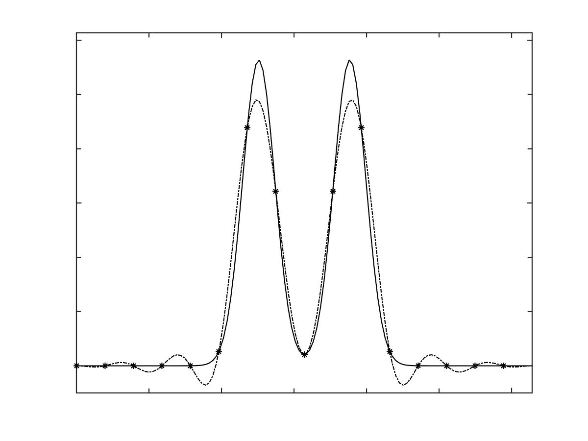
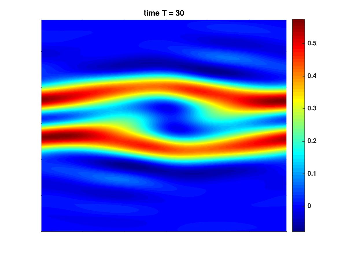
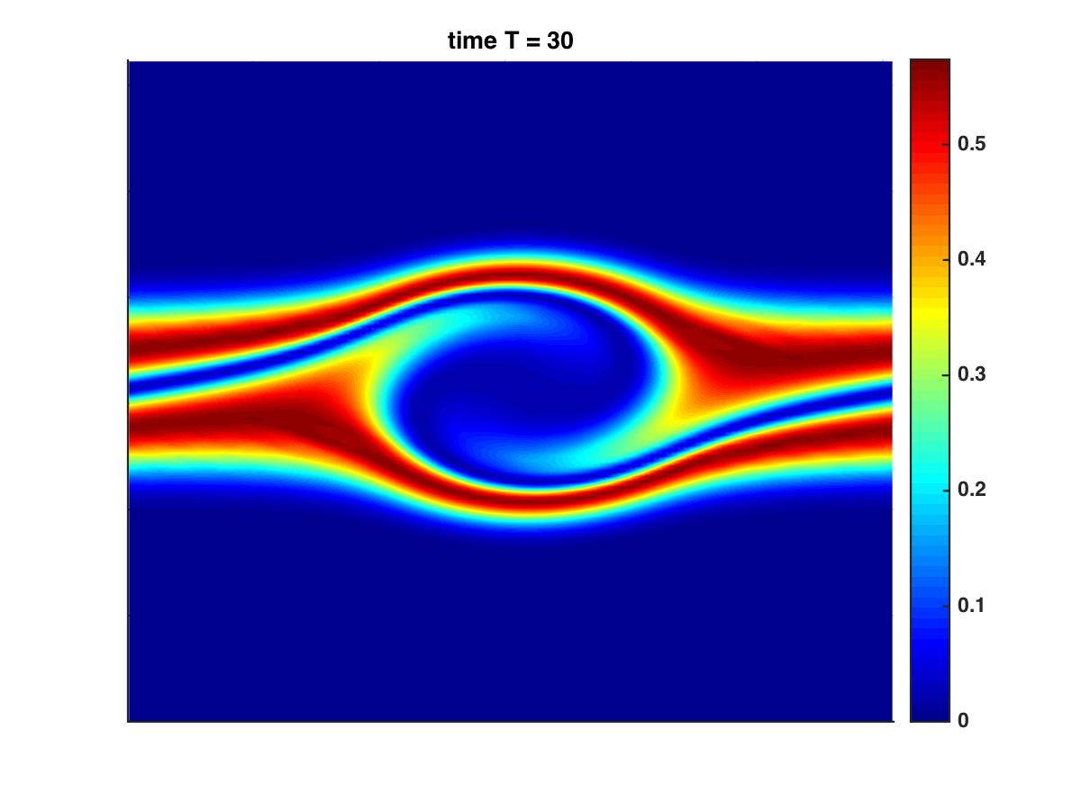
with $\alpha=1/\penalty{\sqrt{8}}$ , $\beta=1$ , $\epsilon=10^{-3}$ , $\kappa=0.5$ . The exact solution is approximated by periodic functions in the variables $x$ and $v$ . We integrate in time up to time $T=30$ using the second-order one-step scheme (72) with timestep $\Delta t=10^{-2}$ . This value is sufficiently small to guarantee stability, since the CFL condition (63) requires $\Delta t$ to be proportional to $1/\max\{N,M\}$ . The results of our simulations are presented in Figures 1, 2, 3 and 4. In particular, in Figure 1, calculations are carried out for different values of the discretization parameters $N$ and $M$ . The plots on the left show the interpolations of the initial solution (82) with respect to the variable $v$ at $x=0$ . Only in the top one there is a little disagreement, since the degrees of freedom look not sufficient, which has, of course, a negative reflection on the final solution. The plots on the right show the corresponding numerical distribution at the final time $T=30$ . The choice $N=M=2^{5}$ already gives reliable approximation results but to completely eliminate the wiggles it is recommendable to increase $M$ up to $2^{7}$ . Note, however, that the global number of degrees of freedom $2^{5}\times 2^{7}=32\times 128$ is rather low.

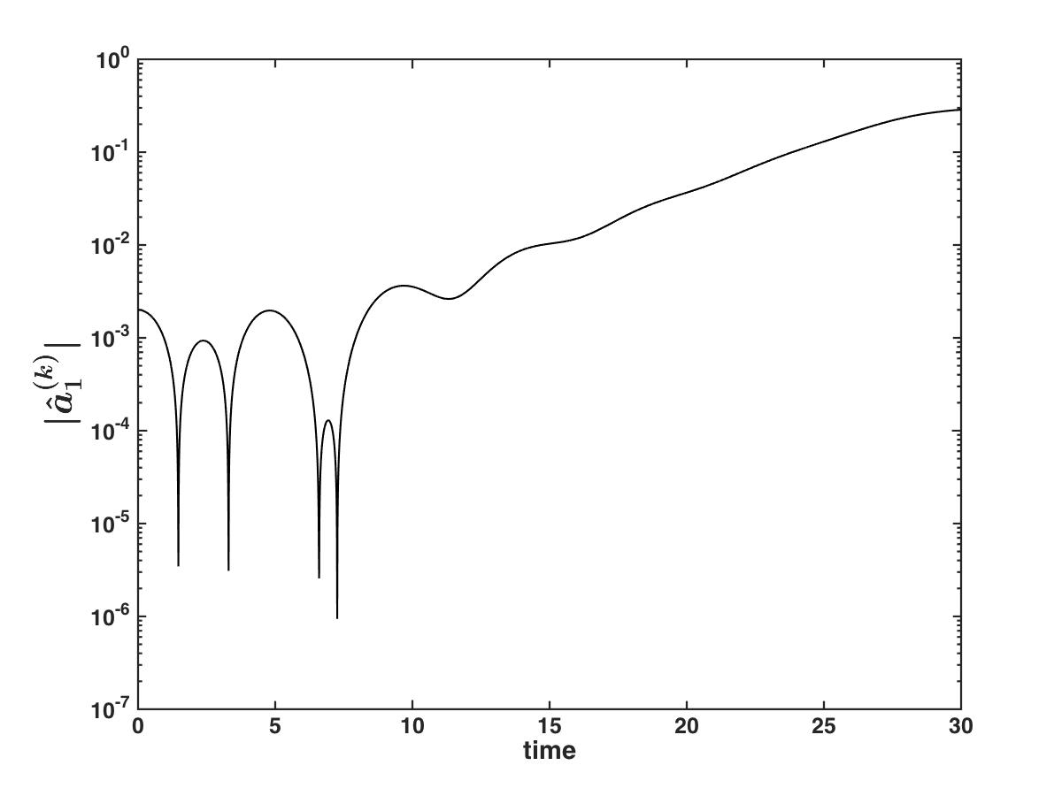
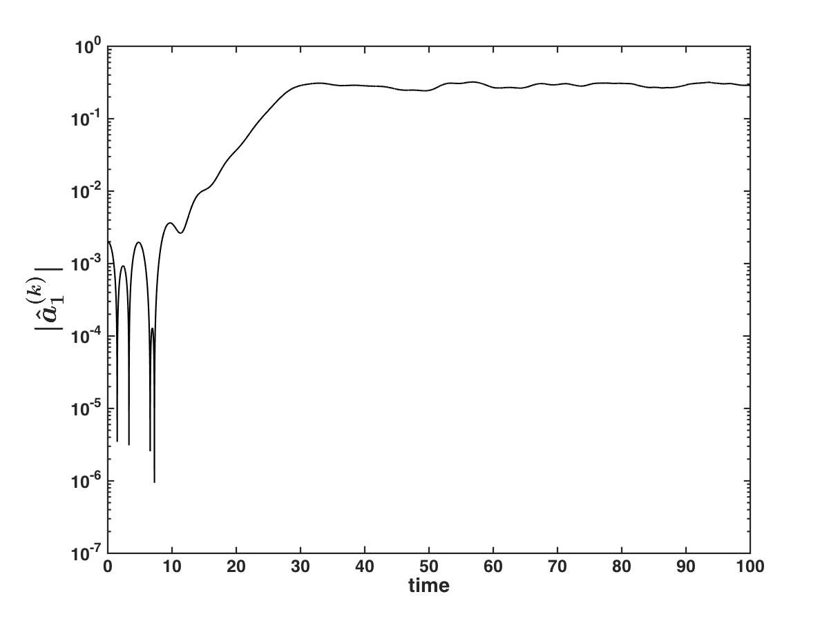
In Figure 2, we plot the time evolution of the ( $\log$ of the) first Fourier mode of the electric field $E^{(k)}_{N}$ in (58), for different values of the discretization parameters. According to (55), this is given by $|\hat{a}_{1}^{(k)}|$ . In particular, the plots show $|\hat{a}_{1}^{(k)}|$ versus time, when $N=2^{5}$ , $M=2^{7}$ , $\Delta t=10^{-2}$ and $T=100$ . These results are in agreement with the behavior expected from the theory. In particular, the slope of the numerical curves in the initial part of the dynamics, where the two-streams instability starts developing, matches well the slope predicted by the linear theory. The stability of the numerical method is shown by the “plateau” up to the final time $T=100$ , which implies that the method is also suitable for long-time integration.

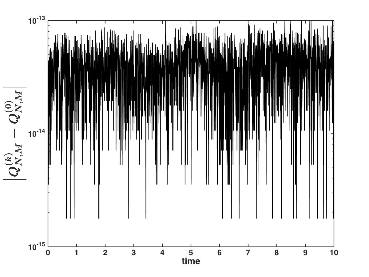
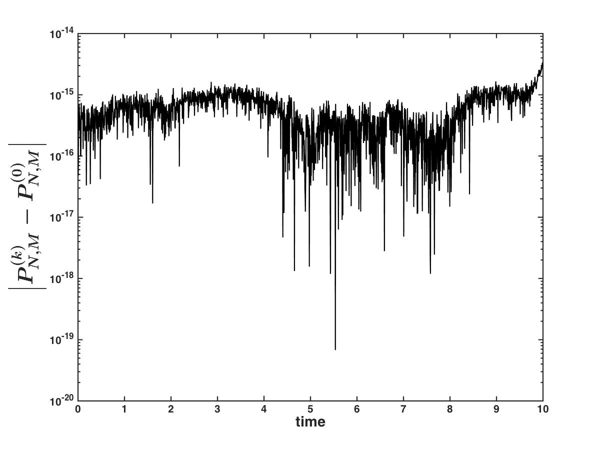
To study the capability of the proposed schemes to preserve physical invariants, we compute the variation with respect to the initial value of the following quantities:

\displaystyle\left|Q^{(k)}_{N,M}-Q^{(0)}_{N,M}\right|,

(83)

and

\displaystyle\left|P^{(k)}_{N,M}-P^{(0)}_{N,M}\right|,

(84)

where the formulas for the discrete number of particles $Q^{(k)}_{N,M}$ and the discrete momentum $P^{(k)}_{N,M}$ are defined in (75) and (78), respectively. The results of this study are given in Figure 3, for different time-marching schemes. The plots show (in a semi- $\log$ diagram) the variation versus time of the number of particles and the momentum, with respect to their initial value, when $N=2^{5}$ , $M=2^{7}$ , $T=10$ and $\Delta t=5\cdot 10^{-3}$ . In the first case (top), the results are excellent (i.e., within the machine precision). In the other cases, a weak growth in time is observed, probably due to the accumulation of rounding errors.

To study the conservation of the total energy, we computed the relative variation of the discrete energy with respect to the initial value:

\frac{\left|\mathcal{E}_{N,M}^{(k)}-\mathcal{E}_{N,M}^{(0)}\right|}{\left|\mathcal{E}_{N,M}^{(0)}\right|},

(85)

where $\mathcal{E}_{N,M}^{(k)}$ is defined in (79). The results of Figure 4 show (in a semi- $\log$ diagram) the behavior of the above quantities for different values of the timestep $\Delta t$ , for $N=2^{5}$ , $M=2^{7}$ and $T=10$ . Here, we implemented the second-order BDF scheme and the third-order BDF scheme. The energy is not perfectly preserved, but the discrepancy decays fast by diminishing $\Delta t$ , according to the accuracy of the method. Indeed, these plots show that the decay rate for the first scheme is quadratic, while that of the second scheme is cubic. It has to be observed that this last method requires a more restrictive condition on the timestep. First of all, this is true because of the smaller domain of stability of BDF high-order methods. Secondly, because in the build-up of the method we trace back the characteristic curves of several multiples of $\Delta t$ (see, for instance, the second relation in (65)).

7.3 Landau damping

In the following numerical tests, the proposed numerical schemes are applied in order to capture the Landau damping phenomenon. Landau damping is a classical kinetic effect in warm plasmas due to the resonance of the particles with an initial wave perturbation. In this classical and well-studied example, the continuous filamentation process in velocity space occurs.

We initialize the electron Maxwellian distribution with a suitable perturbation as follows:

\displaystyle f(0,x,v)=\frac{1}{\sqrt{2\pi}}\left[1+\gamma\cos\left(\kappa x\right)\right]\exp(-v^{2}/2),

(86)

where $\gamma$ is the size of the perturbation and $\kappa$ is the wave-number. For this test, we set $\Omega_{x}=[0,4\pi]$ and $\Omega_{v}=[-10,10]$ . The size of $\Omega_{v}$ ensures that the values attained by $f$ at $v=\pm 10$ are negligible.

7.3.1 Linear Landau damping

In this example, we set $\gamma=0.01$ and $\kappa=0.5$ in (86). Here, the perturbation is small and therefore the plasma behaves according to the linear Landau theory. The solution is computed up to time $T=40$ by using the second-order BDF scheme in time with $\Delta t=2.5\cdot 10^{-3}$ and $N=M=2^{5}$ (left), $N=2^{5}$ , $M=2^{7}$ (right). Figure 5 shows the behaviour in time of the first Fourier mode of the electric field $E^{(k)}_{N}$ (see $|\hat{a}_{1}^{(k)}|$ in (58)) in the $\log$ scale. The recurrence phenomenon starting at time $t\approx 12$ is clearly visible on the left plot, which is due to an insufficient resolution of the velocity domain. This effect can be mitigated by increasing the accuracy of the velocity approximation (we recall that we do not have any artificial dissipation term in these schemes). The plot on the right shows how the method performs when $M=2^{7}$ velocity degrees of freedom are used. A similar behavior has been observed also for the other discretization schemes proposed in this paper.

7.3.2 Nonlinear Landau damping

The initial distribution is again the function in (86), but this time we set $\gamma=0.5$ . The other parameters are the same as in the linear Landau damping. Therefore, a larger amplitude of the initial perturbation is used. In this situation, the Landau linear theory does not hold, because the nonlinear effects become relevant. Nevertheless, several results obtained numerically are available in the literature, since the nonlinear Landau damping is often used to assess the performance of Vlasov-Poisson solvers.

Figure 6 shows the plots at different times for the computation relative to the second-order BDF scheme. In this example, we work with $N=2^{5}$ , $M=2^{7}$ , $\Delta t=2.5\cdot 10^{-3}$ , and $T=40$ . In these plots, the filamentation effect is clearly evident and it is due to the fact that we do not have any explicit artificial dissipation term in the method. The one-step second-order scheme provides identical results when is applied with the same parameters. However, the latter method has less restriction on the timestep than the former one (see also the comments at the end of Section 7.2). Therefore, we can run the same simulation with $\Delta t=5\cdot 10^{-3}$ . The results are shown in Figure 7. Filamentation is still visible, but less evident probably because of some numerical diffusion due to the choice of a larger timestep.

Finally, in Figure 8 we show the first Fourier mode of the electric field $E^{(k)}_{N}$ in the log-scale computed with the second-order BDF scheme for $\Delta t=2.5\cdot 10^{-3}$ , and using $N=2^{5}$ , $M=2^{7}$ on the right and $N=M=2^{5}$ on the left. Again, the different behavior when more degrees of freedom are used for the velocity representation is reflected by the comparison of the corresponding curves.

8 Conclusions

In this work, a class of novel numerical methods for the system of equations of Vlasov-Poisson has been designed, developed, and investigated esperimentally. These methods are based on a spectral approximation in the phase space in a Semi-Lagrangian framework using a first- and a second-order accurate approximation of the characteristics curves. A single-step second-order method is thus obtained without resorting to any splitting of the equations. High-order time discretizations based on the method-of-lines approach are also proposed and studied, which are obtained by adopting second-order and third-order multi-step Backward Differentiation Formulas (BDF). Furthermore, conservation properties have been also investigated. The performance of these methods has been assessed by thorugh a manufactured solution and standard benchmark problems as the two stream instability and the Landau damping.

Refer to caption — Figure 1: Two-stream instability test: interpolation with respect to $v$ of the initial solution (82) at time $t=0$ and $x=0$ (left plots); approximated distribution function in the domain $\Omega=\Omega_{x}\times\Omega_{v}$ at time $T=30$ (right plots). The second-order one-step time-marching scheme is implemented with $\Delta t=10^{-2}$ and $N=M=2^{4}$ (top), $N=M=2^{5}$ (center) and $N=2^{5}$ , $M=2^{7}$ (bottom).

Acknowledgements

The second author was partially supported by the Short Term Mobility Program of the Consiglio Nazionale delle Ricerche (CNR-Italy), which partially funded a scientific visit to the Los Alamos National Laboratory. The third author was supported by the Laboratory Directed Research and Development Program (LDRD), U.S. Department of Energy Office of Science, Office of Fusion Energy Sciences, and the DOE Office of Science Advanced Scientific Computing Research (ASCR) Program in Applied Mathematics Research, under the auspices of the National Nuclear Security Administration of the U.S. Department of Energy by Los Alamos National Laboratory, operated by Los Alamos National Security LLC under contract DE-AC52-06NA25396.

References

[1] T. D. Arber and R. G. L. Vann. A critical comparison of Eulerian-grid-based Vlasov solvers. Journal of Computational Physics, 180:339–357, 2002.
[2] T. P. Armstrong, R. C. Harding, G. Knorr, and D. Montgomery. Solution of Vlasov’s equation by transform methods. Methods in Computational Physics, 9:29–86, 1970.
[3] B. Ayuso, J. A. Carrillo, and C.-W. Shu. Discontinuous Galerkin methods for the one-dimensional Vlasov-Poisson system. Kinetic & Related Models, 4(4):955–989, 2011.
[4] B. Ayuso, J. A. Carrillo, and C.-W. Shu. Discontinuous Galerkin methods for the multi-dimensional Vlasov-Poisson problem. Mathematical Models and Methods in Applied Sciences, 22(12):1250042, 2012.
[5] J. W. Banks and J. A. F. Hittinger. A new class of nonlinear finite-volume methods for Vlasov simulation. IEEE Transactions on Plasma Science, 38(9):2198–2207, Sept 2010.
[6] R. Bermejo. Analysis of an algorithm for the Galerkin-characteristic method. Numerische Mathematik, 60(1):163–194, Dec 1991.
[7] R. Bermejo. A Galerkin-characteristic algorithm for transport-diffusion equations. SIAM Journal on Numerical Analysis, 32(2):425–454, 1995.
[8] C. K. Birdsall and A. B. Langdon. Plasma physics via computer simulation. Taylor & Francis, New York, 1st edition, 2005.
[9] F. Bouchut, F. Golse, and M. Pulvirenti. Kinetic equations and asymptotic theory. Series in Applied Mathematics. Elsevier, 2000. Perthame, B. and Desvillettes, L. Eds.
[10] T. J. M. Boyd and J. J. Sanderson. The Physics of Plasmas. Cambridge University Press, 2003.
[11] J. U. Brackbill. On energy and momentum conservation in particle-in-cell plasma simulation. Journal of Computational Physics, 317:405–427, 2016.
[12] E. Brigham. The fast Fourier transform and its applications. Prentice Hall, 1st edition, 1988.
[13] E. Camporeale, G. L. Delzanno, B. K. Bergen, and J. D. Moulton. On the velocity space discretization for the Vlasov-Poisson system: comparison between Hermite spectral and Particle-in-Cell methods. Part 2: fully-implicit scheme. Computer Physics Communications, in press, 2015.
[14] E. Camporeale, G. L. Delzanno, G. Lapenta, and W. Daughton. New approach for the study of linear Vlasov stability of inhomogeneous systems. Physics of Plasmas, 13(9):092110, 2006.
[15] C. Canuto, M. Y. Hussaini, A. M. Quarteroni, and T. A. J. Zang. Spectral Methods in Fluid Dynamics. Scientific Computation. Springer-Verlag, Berlin Heidelberg, first edition, 1988.
[16] J. A. Carrillo and F. Vecil. Nonoscillatory interpolation methods applied to Vlasov-based models. SIAM Journal on Scientific Computing, 29(3):1179–1206, 2007.
[17] G. Chen and L. Chacon. A multi-dimensional, energy- and charge-conserving, nonlinearly implicit, electromagnetic Vlasov-Darwin particle-in-cell algorithm. Computer Physics Communications, 197:73–87, 2015.
[18] G. Chen, L. Chacon, and D. Barnes. An energy- and charge-conserving, implicit, electrostatic particle-in-cell algorithm. Journal of Computational Physics, 230(18):7018–7036, 2011.
[19] C. Z. Cheng and G. Knorr. The integration of the Vlasov equation in configuration space. Journal of Computational Physics, 22(3):330–351, 1976.
[20] A. Christlieb, W. Guo, M. Morton, and J.-M. Qiu. A high order time splitting method based on integral deferred correction for semi-Lagrangian Vlasov simulations. Journal of Computational Physics, 267:7–27, 2014.
[21] G. H. Cottet and P.-A. Raviart. Particle methods for the one-dimensional Vlasov-Poisson equations. SIAM Journal on Numerical Analysis, 21(1):52–76, 1984.
[22] N. Crouseilles, T. Respaud, and E. Sonnendrücker. A forward semi-Lagrangian method for the numerical solution of the Vlasov equation. Computer Physics Communications, 180(10):1730–1745, 2009.
[23] G. L. Delzanno. Multi-dimensional, fully-implicit, spectral method for the Vlasov-Maxwell equations with exact conservation laws in discrete form. Journal of Computational Physics, 301:338–356, 2015.
[24] J. Dolbeault. An introduction to kinetic equations: the Vlasov-Poisson system and the Boltzmann equation. Discrete Contin. Dyn. Syst, 8(2):361–380, 2002.
[25] F. Filbet. Convergence of a finite volume scheme for the Vlasov-Poisson system. SIAM Journal on Numerical Analysis, 39(4):1146–1169, 2001.
[26] F. Filbet and E. Sonnendrücker. Comparison of Eulerian Vlasov solvers. Computer Physics Communications, 150(3):247–266, 2003.
[27] F. Filbet, E. Sonnendrücker, and P. Bertrand. Conservative numerical schemes for the Vlasov equation. Journal of Computational Physics, 172(1):166–187, 2001.
[28] H. Gajewski and K. Zacharias. On the convergence of the Fourier-Hermite transformation method for the Vlasov equation with an artificial collision term. Journal of Mathematical Analysis and Applications, 61(3):752–773, 1977.
[29] R. Glassey. The Cauchy Problem in Kinetic Theory. Society for Industrial and Applied Mathematics, 1996.
[30] H. Grad. On the kinetic theory of rarefied gases. Communications on Pure and Applied Mathematics, 2(4):331–407, 1949.
[31] R. E. Heath, I. M. Gamba, P. J. Morrison, and C. Michler. A discontinuous Galerkin method for the Vlasov-Poisson system. Journal of Computational Physics, 231(4):1140–1174, 2012.
[32] J. P. Holloway. Spectral velocity discretizations for the Vlasov-Maxwell equations. Transport Theory and Statistical Physics, 25(1):1–32, 1996.
[33] A. J. Klimas. A numerical method based on the Fourier-Fourier transform approach for modeling 1-D electron plasma evolution. Journal of Computational Physics, 50(2):270–306, 1983.
[34] G. Lapenta. Exactly energy conserving semi-implicit particle in cell formulation. Journal of Computational Physics, 334:349–366, 2017.
[35] G. Lapenta and S. Markidis. Particle acceleration and energy conservation in particle in cell simulations. Physics of Plasmas, 18:072101, 2011.
[36] G. Manzini, G. Delzanno, J. Vencels, and S. Markidis. A Legendre-Fourier spectral method with exact conservation laws for the Vlasov-Poisson system. Journal of Computational Physics, 317:82–107, 2016.
[37] G. Manzini, D. Funaro, and G. L. Delzanno. Convergence of spectral discretizations of the Vlasov-Poisson system. SIAM Journal on Numerical Analysis, 55(5):2312–2335, 2017.
[38] S. Markidis and G. Lapenta. The energy conserving particle-in-cell method. Journal of Computational Physics, 230:7037–7052, 2011.
[39] A. Myers, P. Colella, and B. Van Straalen. A 4th-order particle-in-cell method with phase-space remapping for the Vlasov-Poisson equation. SIAM Journal on Scientific Computing, 39(3):B467–B485, 2017.
[40] J. T. Parker and P. J. Dellar. Fourier-Hermite spectral representation for the Vlasov-Poisson system in the weakly collisional limit. Journal of Plasma Physics, 81(2):305810203, 2015.
[41] J.-M. Qiu and A. Christlieb. A conservative high order semi-Lagrangian WENO method for the Vlasov equation. Journal of Computational Physics, 229(4):1130–1149, 2010.
[42] J. W. Schumer and J. P. Holloway. Vlasov simulations using velocity-scaled Hermite representations. Journal of Computational Physics, 144(2):626–661, 1998.
[43] J. Shen, T. Tang, and L.-L. Wang. Spectral Methods. Algorithms, Analysis and Applications. Number 41 in Springer Series in Computational Mathematics. Springer, Berlin, New York, 2011.
[44] E. Sonnendrücker, J. Roche, P. Bertrand, and A. Ghizzo. The semi-lagrangian method for the numerical resolution of the Vlasov equation. Journal of Computational Physics, 149(2):201–220, 1999.
[45] A. Staniforth and C. J. Semi-lagrangian integration schemes for atmospheric models – a review. Monthly Weather Review, 119(9):2206–2223, 1991.
[46] E. T. Taitano, D. A. Knoll, L. Chacon, and G. Chen. Development of a consistent and stable fully implicit moment method for Vlasov–Ampère particle in cell (PIC) system. SIAM Journal on Scientific Computing, 35(5):S126–S149, 2013.
[47] J. Vencels, G. Delzanno, G. Manzini, S. Markidis, I. Bo Peng, and V. Roytershteyn. SpectralPlasmaSolver: a spectral code for multiscale simulations of collisionless, magnetized plasmas. Journal of Physics: Conference Series, 719(1):012022, 2016.
[48] J. Vencels, G. L. Delzanno, A. Johnson, I. Bo Peng, E. Laure, and S. Markidis. Spectral solver for multi-scale plasma physics simulations with dynamically adaptive number of moments. Procedia Computer Science, 51:1148–1157, 2015. International Conference On Computational Science, {ICCS} 2015 Computational Science at the Gates of Nature.
[49] S. Wollman. On the approximation of the Vlasov-Poisson system by particle methods. SIAM Journal on Numerical Analysis, 37(4):1369–1398, 2000.
[50] S. Wollman and E. Ozizmir. Numerical approximation of the one-dimensional Vlasov-Poisson system with periodic boundary conditions. SIAM Journal on Numerical Analysis, 33(4):1377–1409, 1996.