Balanced Random Survival Forests for Extremely Unbalanced, Right Censored Data
Abstract
Accuracies of survival models for life expectancy prediction as well as critical-care applications are significantly compromised due to the sparsity of samples and extreme imbalance between the survival (usually, the majority) and mortality class sizes. While a recent random survival forest (RSF) model overcomes the limitations of the proportional hazard assumption, an imbalance in the data results in an underestimation (overestimation) of the hazard of the mortality (survival) classes. A balanced random survival forests (BRSF) model, based on training the RSF model with data generated from a synthetic minority sampling scheme is presented to address this gap. Theoretical results on the effect of balancing on prediction accuracies in BRSF are reported. Benchmarking studies were conducted using five datasets with different levels of class imbalance from public repositories and an imbalanced dataset of 267 acute cardiac patients, collected at the Heart, Artery, and Vein Center of Fresno, CA. Investigations suggest that BRSF provides an improved discriminatory strength between the survival and the mortality classes. It outperformed both optimized Cox (without and with balancing) and RSF with an average reduction of 55% in the prediction error over the next best alternative.
keywords
balanced random survival forests, class imbalance, ST-elevated myocardial infarction, survival analysis, synthetic minority.1 Introduction
Mortality prediction, risk stratification, and key biomarker identification in acute and high-risk patients are prominent tasks in healthcare survival analysis (Amsterdam et al., 2014; O’Gara et al., 2013). Their importance is further accentuated while dealing with life-threatening conditions such as acute cardiovascular diseases and cancer. An accurate prediction of the adverse pathologies can allow risk-calibrated interventions for better management of the outcomes. Survival analysis models are one of the key tools which provide decision support to the physicians not only for intervention selection but also for identifying high-risk patient and for patient counseling/consent for intervention (Furnary et al., 1996; Dankner et al., 2003). Nonetheless, the limited accuracy of such survival models which guide critical life-and-death decisions remains a major concern.
Currently, most of the real world applications employ the Cox proportional hazard model for mortality prediction (CPH) (Harrell Jr, 2015). For a given covariate vector, (capturing the various biomarkers in the present context), CPH reduces the estimation of hazard function at a time , , for an individual into a regression problem of the form , where is an unknown vector of regression coefficients. The popularity of CPH rises from its semi-parametric nature, which does not require any distributional assumption of the baseline hazard function, , to estimate . Nonetheless, selecting a wrong can significantly change the result (Ohno-Machado, 1997). Additionally, the CPH model makes certain restrictive assumptions, many of which do not hold in real life scenarios. One such assumption is a constant hazard ratio between any two observations at every time instant, . It also does not take into account the missing predictors, the nonlinearity of the exponential factor, interdependence among observations, and is known to have an inherent bias and high generalization error (Binder, 1992; Snedecor and Cochran, 1989; Pan and Schaubel, 2008).
Recent innovations in the sensor technologies for gathering a rich collection of clinical biomarkers, together with advent of innovative methodologies for predicting time-to-event, based on advanced machine learning techniques have opened new possibilities to overcome the limitations of CPH models (Belle et al., 2011; Ishwaran et al., 2008), many of which address the limitations of CPH model. One such method is random survival forest (RSF) (Ishwaran et al., 2008). RSF is a non-parametric approach to right-censored survival analysis based on a Breiman’s ensemble tree, random forests model. In Breiman’s random forests, a tree is grown using independent bootstrapped samples with a different set of biomarkers at each node, randomly selected from . This two-way randomization improves both bias and variance of the resulting random forests ensemble. Its performance is at least comparable to that of the state-of-the-art machine learning methods, such as boosting and support vector machine (Ishwaran and Kogalur, 2010). Additionally, RSF effectively imputes the missing data—a common problem in healthcare datasets. RSF inherits the robustness and desirable properties (increased accuracy, minimized bias, and variance) of random forests model to the survival analysis. Recent works using RSF for survival data have shown improved results as compared to the CPH models and are getting popular as a survival analysis tool (Hsich et al., 2011; Mogensen et al., 2012).
Nonetheless, the characteristics of the survival data pose significant challenges to RSF. Besides right-censoring, the presence of extreme imbalance between the censored and the mortality classes with as low as 2-10% data in the minority is a commonly occurring, yet often ignored aspect. Due to the contemporary clinical practice and infrastructure across the US, acute cardiac and other life-threatening diseases are mostly treated in small tertiary care hospitals and, as a result, the cohort size tends to be small, further exacerbating the challenge. Balancing is an essential step in maximizing the utility and improved mortality prediction performance. Although data balancing is important, only a few works focuses on addressing class imbalance from a survival analysis context (Chia et al., 2012). In this work, we propose a balanced random survival forests (BRSF), which integrates RSF with a synthetic data balancing scheme. We present some key theoretical result on the effect of class imbalance on improving model’s predictive performance from a survival analysis context. The performance of BRSF was with RSF as well as, an optimized CPH model and its balanced counterpart. Here, optimized CPH refers to the CPH model where overfitting errors are minimized through predictor selection. All models are assessed on a set of 5 benchmark datasets each representing a different degree of class imbalance, as well as a dataset gathered at the Heart, Artery, and Vein center of Fresno from 267 acute cardiac STEMI (ST Elevated Myocardial Infarction) subjects after they underwent cardiac revascularization therapy. The paper reports the following three contributions, namely, the development of BRSF approach to address the challenges with high class imbalance and small data size in survival analysis, establishment of theoretical results on how data balancing can improve model prediction, and comparison of the performance of BRSF models relative to that of the other contemporary survival models in multiple scenarios with high data imbalance, which collectively can enhance informed treatment decision for healthcare providers.
The remainder of this paper is organized as follows. We describe the BRSF modeling approach and delineate the performance comparison measures in Section 2. In Section 3, we provide the details for the survival datasets used in this paper and the comparative results obtained before and after addressing the class imbalance. Finally, Section 4 summarizes the paper and discuss some future work for effectively balancing the survival data.
2 Balanced RSF for Mortality Prediction
The BRSF model consists of two main aspects, namely, the tree-based random survival forest modeling, and the class balancing methodology, as presented in the following subsections.
2.1 An Overview of Random Survival Forests
Growing a random survival forest, can be thought of as a hierarchical procedure which initializes by randomly drawing bootstrap samples from the training data consisting of samples, each with predictors (here, biomarkers), and growing a survival tree for each of the drawn samples (see Figure 1). The bootstrap samples are invariably extracted from right-censored survival data. For analyzing survival data, follow up time and associated right censoring are important considerations. Right-censored survival data of individuals is the collection of values in a set, , where the subscript is the patient index, and are independent and identically distributed (i.i.d.) biomarkers of patient . Let and be the true event (death) and censoring time, respectively for subject . The observed survival time is then given as , and is the binary censoring status specified as follows: given the vector of biomarkers, , an individual is said to be right-censored if , i.e., or else the individual is said to have experienced death at time at time .
Here, the construction of a survival tree, from the bootstrapped data begins with a random selection of out of possible biomarkers in . Although we used the suggested, (Ishwaran et al., 2011; James et al., 2013), the value of depends on the number of available biomarkers and is data specific. Previous studies have even shown good performance with , care must be taken as an increase in tend to result in correlated trees (Breiman, 2001). Next, all the bootstrapped samples are assigned to the root node, i.e., the topmost node of the tree. The root node is then split into two daughter nodes, and each of thus-generated daughter nodes is then recursively split with progressively increasing within-node homogeneity. Now, for any parent node with predictors, the split on a given predictor, is of the form and . Here, conventionally takes values at the midpoint of consecutive distinct observations of corresponding to the individuals in the parent node being split (Segal, 1988). Thus, has at most one less than the parent node size values.
Let be unique event (death) times at the parent node, , and and denote the number of deaths and individuals who are alive (at risk) in the daughter node at time . It follows that individuals had survival time of less than , and individuals had a greater survival time. For a split using biomarker and its splitting values , the goodness-of-split is measured using a log-rank statistic (Segal, 1988) represented as:
| (1) |
Here, Equation 1 measures the separation between two daughter nodes. Hence, the best split at a node is determined by the biomarker and its value at the cut point such that . Algorithm 1 presents the procedure to select and for any given parent node with distinct values of .

Figure 1 presents a pictorial representation of a RSF and the log-rank split procedure presented in Algorithm 1. Trees are grown until no new daughters can be formed due to a stopping criterion of a minimum of unique deaths (Ishwaran et al., 2008). Here, we used . At this point, there are terminal/leaf nodes in the tree, . Now, let be one of the terminal nodes with distinct event times, . Following the notations introduced above, the cumulative hazard function (CHF) for the node as given in Equation (2) here, is the Nelson-Aalen estimator for the patients in at time (Borgan, 2005).
| (2) |
For an individual with a vector of biomarkers , the CHF is same as that of the terminal node it belongs to, i.e. . However, due to bootstrapping (sampling with replacement) an individual can be present in several bootstrap samples and hence in several trees. Thus, to obtain an out of bag (OOB) ensemble CHF, for individual at time , we calculate the average of the CHFs for all such trees in which is an OOB sample. For the tree with CHF , let be 1 if is an OOB data for and 0 otherwise, then the OOB ensemble CHF for that individual is given by:
| (3) |
In practice, hazard functions for training are calculated on the OOB data to avoid an optimistic bias in the result. For each bootstrap sample about one-third of the data is left for OOB. The main steps of the RSF algorithm are summarized in Algorithm 2.
Now, we discuss some of the notable features of the RSF. First, introducing the two-fold randomization both by bootstrap samples as well as by candidate variables reduces the generalization error and provides RF and its related method RSF an edge over the traditional approaches. The value of can be estimated using the generalization error. Since the generalization error approaches a limiting value with increasing number of trees after a point adding more trees does not add to the increased accuracy of the forest (Breiman, 2001). We selected trees for our analysis.
Second, RSF helps in solving another key issue of missing data. As is the case for most of the real data, missing values are generally present and severely affect the error estimation. RSF uses an adaptive tree imputation method at each parent node to impute missing data (predictors and outcomes) before the node is split. For the training data at a node, , imputation for the missing values of the biomarker works by randomly drawing from the empirical distribution, of “in-bag” non-missing set of values for at node . The daughter node thus formed does not contain any missing data. However, for robust results, the imputed values are reset to missing in the daughter node and the imputation is iteratively repeated at every node until the terminal node is reached. Now, the final summary imputed value for the missing biomarkers for subject is the average (across the forest) of its “in-bag” imputed values obtained from the terminal nodes in which the subject is present. In case the biomarker is not continuous, most frequently occurring “in-bag” imputed value is considered. Imputation for the missing values in the test data proceeds in the same way, however, the missing values are drawn from the original distribution, from the training data (Ishwaran et al., 2008). Third, it may be noted that with the assumption of discrete feature space, an RSF has shown to converge uniformly to the true population survival function (Ishwaran and Kogalur, 2010). This demonstrates the consistency of the RSF for right-censored survival analysis. RSF indeed has several merits and might provide good predictions (measured in terms of the metrics presented in subsection 2.2), but real life survival data with extreme imbalance coupled with small data sizes often make accurate prediction very challenging. We discuss the balancing methodology used to address this limitation of the RSF in subsection 2.3.
2.2 Performance Measures
In the automated prognostics and decision support practice, where data drives the critical decision-making, robustness of the model is of utmost importance. Recently, there have been vigorous debates on the effectiveness of the performance measures and on the efficacy of one measure over the other (Ishwaran et al., 2011). Here, we compare the performance of BRSF relative to contemporary survival models based on three of the most popular metrics in survival analysis literature. These are concordance index, prediction error curves, and Integrated Brier score. Further, an accurate estimation of prediction error with limited data is a challenging task, therefore we use 10 fold cv scheme to calculate each of these measures to minimize bias for the test data, and to improve precision in the scenario of induced variance due to the data-driven steps in model building and validation measure.
2.2.1 C-index
Harrell’s concordance index or C-index (Harrell et al., 1982) is perhaps the most popular measure of model’s discriminative strength in the right-censored survival analysis literature. In order to compute C-index, we first need to define permissible cases and concordant pairs. To account for the censoring, the set of permissible cases consists of all possible pairs of individuals, and in the data, but with two exceptions: 1) the ones in which shorter survival time is censored, and 2) when , but neither of and has the event (death). Now, for any randomly selected pair out of the permissible cases, a pair can be concordant or partially concordant depending on their values of ensemble hazard, event time, and censoring status. For example, for a pair with distinct ensemble hazard and event times, a concordance value to 1 is assigned if the predicted risk (in terms of ensemble CHF) is greater for the individual that experiences death first i.e., . Here denote all the unique event times in . For each pair in , the concordant pairs and their assigned concordance values can be given as:
Then the C-index can be expressed as the ratio of the sum of concordance values and the total number of permissible pairs as:
Since represents the classification probability of the model, a higher value is desirable. A value of 50 is essentially no better than random guessing.
2.2.2 Prediction error curves (PEC)
We use PEC to capture a model’s prediction of the survival probability for the test data at different time points. In the absence of censoring, PEC for an individual in the test data is an expectation of the squared difference between the true survival status and predicted survival probability of at time with biomarkers . However, censoring introduces bias in the population average of PEC. The introduction of inverse probability of censoring weight (IPCW) by Gerds and Schumacher (2006) provides a versatile measure to overcome this limitation by weighting the squared residuals using IPCW. Given the survival data , let the test dataset contain independent and identically distributed replicates of , where . With the observed status for subject , and its predicted survival status , the prediction error or Brier score at time is given as:
| (4) |
In Equation 4, the inverse probability of the censoring weights is estimated as (Gerds and Schumacher, 2007):
where denotes the estimated conditional survival function of the censoring time. Here, the prediction error in Equation 4 is estimated from test data via a 10 fold cv scheme. The aim here is to give the averaged prediction error at every time point in the test data. We also use survival probability plots of individuals in the test data at all event time points to show the predicted survival probability of the balanced and unbalanced models.
2.2.3 Integrated Brier Score (IBS)
IBS consolidates the PEC estimates over all time points and is defined as:
Where is the total time span for which the prediction errors can be estimated. Since it is an average of the PEC, we also desire small error. A value of 0.25 means that irrespective of their risk status, the model predicted risk for all the individuals whereas, a value of indicates perfect prediction.
2.3 Class Balancing Scheme
The survival data, in general, has highly imbalanced classes. This extreme imbalance results in suboptimal performance of the survival models, whether it be CPH or RSF. Further, the size of the survival is another concern as the data obtained from the tertiary care hospitals providing acute care are often small, which further aggravates the issue (Japkowicz and Stephen, 2002). Several balancing methodologies have been proposed in the literature to address class imbalance and have been applied in the context of random forests (Chen et al., 2004), albeit, with very limited consideration in survival analysis. In this work, we emphasize the importance of balancing the survival data in order to develop an accurate prediction model.
Data balancing has been addressed using resampling methods such as under-sampling the majority class until their numbers are reduced or made equal to the number of samples in the minority class or over-sampling the minority class until its size is as large as the majority class. Prior investigations suggest that over-sampling does not improve the minority class representation significantly and under-sampling is a better approach than over-sampling (Japkowicz, 2000; Chawla et al., 2002). Unfortunately, various real-life scenarios, including the present context where data is obtained from tertiary care hospitals, only limited samples are available. In such cases, under-sampling leads to an unwanted decrease in the training dataset and is not a feasible option. The imbalance shown in Figure 3(a) is representative of the STEMI dataset which consists of tracking 267 patients for their mortality over a period of 1 year, out of which 62 (only 23%) belong to the minority class (i.e., suffered mortality). This led us to explore a synthetic generation of minority class samples without resorting to excessive under-sampling. We adopt the synthetic minority over-sampling technique (SMOTE) proposed by Chawla et al. (2002).

This synthetic generation process proceeds by randomly selecting a minority and its nearest minority class neighbors. The value of is determined by the amount of over-sampling needed. Let be the feature vector representing the biomarkers for the selected minority and be the feature vector of a randomly chosen neighbor, then a new synthetic minority, is generated in the biomarker (feature) space as follows:
| (5) |
where, is a uniform random variable. Thus, the synthetically generated data can be interpreted as a randomly sampled point along the line segment between the two minority samples in the biomarker space. Depending on the extremity of imbalance, a sample can be created along with all the lines joining the selected minority sample and its neighbors. Representation of this scheme in two-dimensional feature space is shown in Figure 3.

The following results outline the impact of extreme imbalance on RSF, and the effect of balancing in improving survival prediction. Proving any result related to the hazard estimation requires establishing the form of true cumulative hazard function. As defined above, are the actual survival times for the individuals. These survival times are assumed to be dependent with common continuous marginal distribution function . The underlying true cumulative hazard function is then given by (Cai, 1998). In the remainder of this section, we first prove that the hazard estimates and are underestimations of the true hazard whenever the minority class is mortality and an overestimation in case the survival/censored class is minority. Subsequently, we establish the theoretical results for improvement in the prediction error after balancing.
Proposition 1.
Let and be the number of censored and mortality samples in and , be the cumulative hazard function estimated for the censored and mortality nodes respectively. Then for the mortality node is an underestimation, i.e., for and overestimation for .
These results are based on two important aspects of the RSF construction, namely, 1) daughter node size constraint, and 2) terminal node hazard estimation (see Section 2.1). The daughter node size constraint states that each of the resulting daughter nodes after the split must contain a minimum of unique deaths. The splitting terminates if the criterion is not satisfied. When the size of the mortality class is very small as compared to the censored class, the tree terminates prematurely and might result in decision region to be smaller and biased. As a default setting of the RSF, a minimum of unique deaths needs to be present in each of the daughter nodes. Since each case in a particular terminal node has the same hazard function as the cumulative hazard function of the constituting terminal node, the hazard for the death samples in the terminal node with censoring majority is lower. Since the mortality samples are originally smaller in number this results in underestimation of their overall hazard function.
Balancing further results in an improvement in the prediction error. This improvement in the prediction error (in terms of Brier score) from to after balancing can be stated using the following proposition which considers the present context where the number of the mortality (minority) class samples are much fewer that that of the survival (majority) class. Here we assume and an almost perfect split (for simplicity of calculation):
Proposition 2.
For , let and be the surviving and the mortality class size, and the Brier score (BS) before and after balancing, respectively, and be the minimum number of unique death (mortality class) samples needed to present in the leaf nodes of an RSF tree. Assuming an almost perfect split with samples in the mortality node and samples in the censoring node (details in Appendix), can be approximated as:
The result can be similarly derived for the case when . This proposition leads us to our next result on how the unbalanced Brier score or prediction error related to the balanced error.
Corollary 1
Let be the Brier scores before and after balancing the class sizes, then .
This Corollary establishes that after addressing the class imbalance, the prediction error decreases. Proofs for the Proposition 1 & 2, and Corollary 2.3 are provided in the Appendix of this paper.
3 Case Studies
We apply BRSF on six different real-world survival datasets with varying degree of class imbalance. The use of real-data for BRSF’s comparative analysis is to ascertain its relative effectiveness and suitability in the real world decision makings. Our main point of focus in this study is the STEMI dataset obtained from Heart, Artery, and Vein Center of Fresno. This dataset
3.1 Performance Evaluation on Benchmarking Datasets
Five of the six datasets (except the STEMI dataset) used in this study were obtained from online repositories, each with a different level of imbalance. These 5 datasets consists of survival analysis data for acute diseases such as lung cancer (veteran and lung datasets), a rare and fatal chronic liver disease (pbc dataset), acute stroke in patients with atrial fibrillation (COST dataset), and plasma cell immune disorder which may result in malignancy (mgus dataset). A summary of the class proportions in all the datasets for the censored and the event classes is given in Table 1.
| Class proportions | |||
|---|---|---|---|
| Dataset | Total | Censored | Event |
| veteran (Kalbfleisch and Prentice, 2011) | 137 | 9 | 128 |
| mgus (Kyle, 1993) | 241 | 16 | 225 |
| COST Jørgensen et al. (1996) | 518 | 114 | 404 |
| STEMI (Sawant et al., 2013) | 267 | 205 | 62 |
| lung (Loprinzi et al., 1994) | 228 | 63 | 165 |
| pbc (Ishwaran and Kogalur, 2007) | 418 | 257 | 161 |
- *
Minority class represented in red
Most of the datasets contained several missing values which were then imputed using adaptive tree imputation (Ishwaran et al., 2008). To compare CPH and RSF and to determine the effect of balancing on these models, we use the C-index and IBS measures described in subsection 2.2. Table 2 presents the average C-index and IBS scores for CPH, balanced CPH (BCPH), RSF, and BRSF obtained via a 10 fold cv scheme. The best model obtained for both C-index and IBS are shown in blue. As evident from this Table, BCPH and BRSF consistently perform better than their unbalanced counterparts. Additionally, the performance of BRSF supersedes all other models.
| Model | |||||
|---|---|---|---|---|---|
| Dataset | Error measure | CPH | BCPH | RSF | BRSF |
| veteran | C-index | 59 (0.24) | 58 (0.21) | 61 (0.11) | 77 (0.04) |
| IBS | 0.15 (0.04) | 0.14 (0.03) | 0.15 (0.05) | 0.09 (0.02) | |
| mgus | C-index | 71 (0.05) | 89 (0.021) | 69 (0.07) | 88 (0.02) |
| IBS | 0.13 (0.02) | 0.06 (0.01) | 0.14 (0.02) | 0.04 (0.01) | |
| COST | C-index | 69 (0.03) | 76 (0.03) | 64 (0.04) | 85 (0.01) |
| IBS | 0.17 (0.01) | 0.15 (0.01) | 0.18 (0.02) | 0.06 (0.01) | |
| lung | C-index | 61 (0.09) | 70 (0.04) | 59 (0.09) | 76 (0.03) |
| IBS | 0.18 (0.01) | 0.13 (0.01) | 0.18 (0.02) | 0.08 (0.01) | |
| pbc | C-index | 77 (0.09) | 79 (0.02) | 78 (0.08) | 83 (0.02) |
| IBS | 0.14 (0.02) | 0.12 (0.01) | 0.13 (0.02) | 0.07 (0.01) |
- *
Numbers inside the bracket represents standard deviation across 10 fold cv
Given this result, we now focus on the STEMI dataset obtained for the Heart, Artery, and Vein Center of Fresno to do the further in-detail analysis. A concise description of the study design and biomarkers for this data is provided in subsection 3.2 and the results of these analyses are then discussed in the subsequent sections.
3.2 STEMI Dataset Study Design and Biomarkers
The study cohort for the STEMI dataset consisted of 278 consecutive patients. The patients had electrocardiographic criteria for STEMI and a presumed diagnosis for acute coronary syndrome at the time of presentation to the emergency room of a tertiary care hospital in central California, USA. Electrocardiographic, radiographic, and basic laboratory investigations were obtained at the time of presentation and an emergent coronary angiography was performed. Patients underwent coronary artery bypass grafting (CABG) or primary percutaneous coronary intervention. Enrollment into the study began in January 2007 and patient were followed for one year until January 2008. A detailed design of this retrospective study has previously been published (Sawant et al., 2013). We focused primarily on patients (187 male and 80 female) who did not have preexisting left bundle branch block or paced rhythm on ECG. Dataset consisted of a large set () of biomarkers. These biomarkers included therapy provided, physiological and anatomical variables such as age, gender, ethnicity, BMI, ECG criteria, the occurrence of cardiac arrest during admission, troponin levels at the time of discharge, Brain Natriuretic Peptide (BNP) levels, and clinical risk measures such as TIMI index, Mayo Clinic risk score etc. along with the previously mentioned laboratory measurement. The dataset had ethnically diverse population including Black, Caucasian, and a high percentage of representative minority populations such as American Indian, Asian and Hispanics thus somewhat offsetting the demerits of small data size. Mortality data were obtained either from either the hospital, California Department of Public Health (CDPH) or Social Security Death Index records. To avoid any confounding effects of loss to follow-up, and accurate determination of the cause of the death, an all-cause mortality was selected as a primary endpoint instead of disease-specific mortality. Out of the 267 patients,62 patients died in one-year duration (representing the minority class for this dataset).
3.3 Performance Evaluation on STEMI Dataset
We again evaluate the CPH, BCPH, RSF, and BRSF models with respect to C-index and IBS scores obtained via 10 fold cv on the STEMI dataset. As can be seen from the Table 3, presenting the average performance of the models,the balanced models perform better than their unbalanced counterparts with an exception of balanced CPH which is statistically the same as unbalanced CPH in terms of C-index. In terms of IBS, BRSF performs significantly better with a improvement than the unbalanced RSF. In Figure 4, we show this improvement in IBS score by plotting prediction error or Brier score at various times points of the 1 year study duration for one of the 10 folds of cv trials.
| Model | ||||
|---|---|---|---|---|
| Error measure | CPH | BCPH | RSF | BRSF |
| C-index | 80 (0.12) | 79 (0.05) | 82 (0.08) | 82 (0.06) |
| IBS | 0.18 (0.07) | 0.12 (0.04) | 0.17 (0.06) | 0.08 (0.01) |
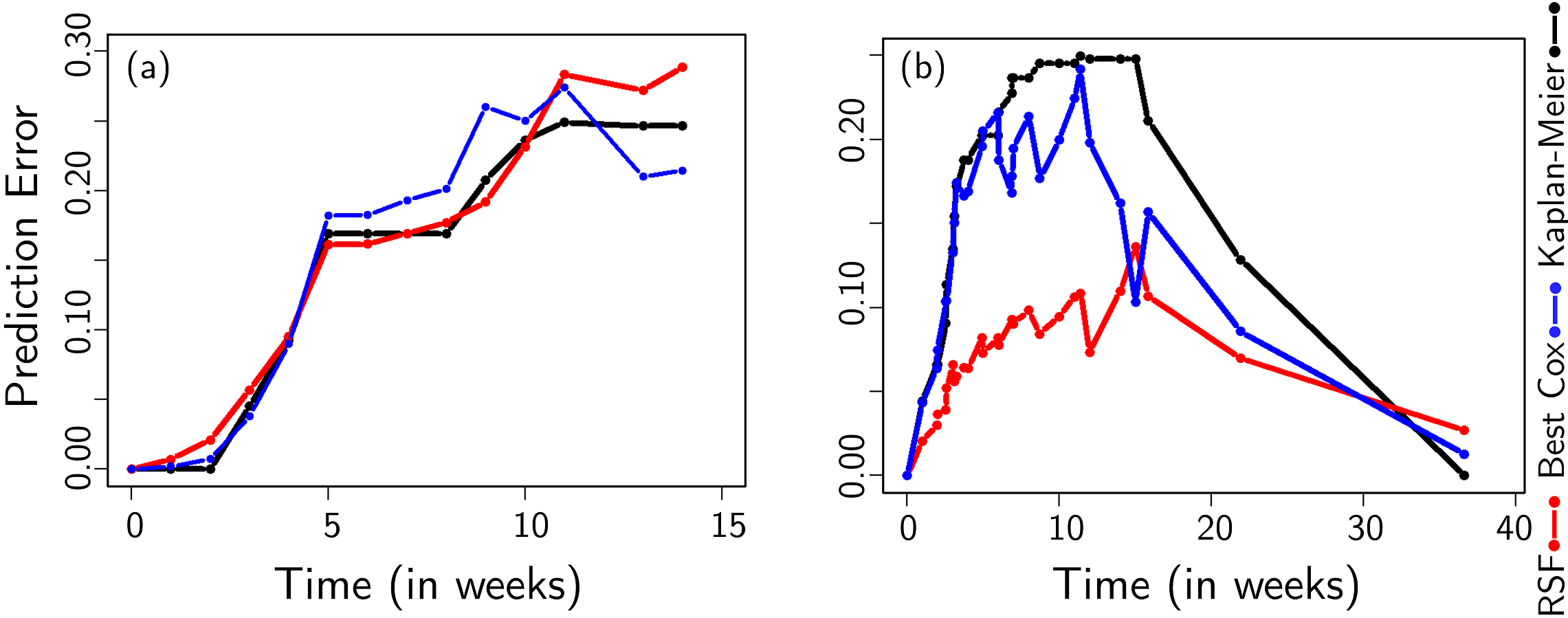
Further, this performance can be better represented in terms of the survival curves. The survival probability for the STEMI test samples in the unbalanced and balanced data are shown in Figure 5 (a) and (b) respectively. When the classes are balanced not only their separability (i.e. higher survival probability for the false event and lower for the true event) increases the survival/hazard estimates for the minority samples also improves. The survival probability plots for all other datasets (Table 1) are shown in the Appendix Appendix A. Investigation of the Effect of Class Balancing on Survival Analysis demonstrating similar improvement in the survival probability estimates. Additionally, Figure 6 summarizes the 10 fold cv IBS for all the datasets. There was an overall improvement of in the C-index and in the IBS score from RSF to BRSF.


We obtained 7 best biomarkers based on backward selection. Their OOB error was 15.8% compared to 18% with all 150 predictors. It turns out these predictors have high importance per both Breiman’s variable importance (VIMP) (Breiman et al., 1984) and Ishwaran et. al.’s minimal depth (MD) scores (Ishwaran et al., 2010) (see Table 4). From a physiological standpoint, these covariates are among the most significant biomarkers of survival during acute cardiac diseases, as elaborated in the following paragraphs.
| Biomarkers | |||||||
|---|---|---|---|---|---|---|---|
| Ranks | Disch | MCRS | Cron | GRACE | MCRS | CHF | ACS |
| (statistics) | Trop | MS | DC | Prob | MACE | in1yr | in1yr |
| MD | 1(8.16) | 2(8.39) | 3(8.53) | 4(8.75) | 7(9.28) | 8(9.30) | 12(9.69) |
| VIMP | 9(0.01) | 3(0.02) | 1(0.02) | 8(0.01) | 7(0.01) | 4(0.02) | 5(0.02) |
We graphically explored the relation of thus selected most important biomarkers (top 7) with the survival probability using partial dependence plots and verified their physical meaning and significance. In a survival setting, a partial dependence plot represents the response corresponding to the biomarker of interest at a particular time by averaging out the joint effect of remaining biomarkers (Friedman et al., 2001; Ehrlinger, 2016). In Figure 7, the two curves corresponding to each of the biomarkers shows the trend of survival probability with changing value of the biomarker at and week for randomly chosen subjects. It shows nonlinearly-decreasing survival probability with increasing value of “CronDC”, “MCRS-Mortality Score(MS)”,“MCRS-MACE”, “CHFin1yr”,“GRACEProb”, “DischTrop” (NOTE: Since all plots have same vertical axis limits, some dominant non-linear relationships make curves for “GRACEProb” and “MCRS-MS” appear flatter than they actually are). For all the biomarkers, we can see the decreasing survival probability with increasing time (“blue” line for week is below the “green” line for week). The variables selected were evaluated by a cardiologist to have a significant physical correlation with the prediction of mortality.
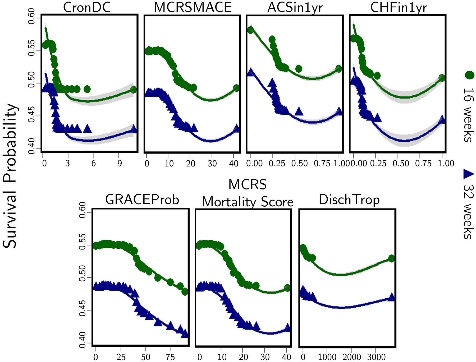
In particular, the DischTrop (discharge troponin) biomarker, recording the troponin levels during the patient discharge is studied as a primary diagnostic component (Ottani et al., 2000; Croal et al., 2006). Troponin is a protein released during myocardial infarction. A higher level of troponin indicates more damage to the cardiac muscle. Figure 8 is a visualization of survival probability trend with varying DischTrop level across the mortality and survival samples. Patients with higher level of troponin content during the discharge shows to have lower survival probabilities. Though application of machine learning algorithms, in particular, RF based approaches are often criticized for their lack of interpretability in real-world data, the variable and partial dependence plots for all the biomarkers can provide insightful information on their relationship with mortality. Consequently, the proposed technique can be used can be used by a healthcare practitioner as an analytical analysis tool to achieve improved throughput and accuracy.

4 Conclusions
In this paper, we have introduced a BRSF model for survival analysis which is expected to address the limitations of both traditional methods such as CPH and newer methods such as RSF in handling extremely imbalanced datasets. The theoretical results as well as extensive experimental analysis presented in this paper demonstrate the superiority of BRSF method in terms of various performance measures. Empirical studies with datasets suggest a improvement in IBS score. Although class imbalance has been extensively studied in the machine learning literature, its theoretical analysis and application in the domain of survival analysis still remain largely unexplored. Pertinently, this is among the first investigations into the effect of class imbalance on the performance of survival models. Specifically, the theoretical results on performance improvement accrued from balancing the RSF models as well as the detailed empirical studies can lead to further improvements to the algorithms for RSF as well as more optimized balancing strategies. This study may provide a foundation for further knowledge discovery and subsequent improvement in survival analysis—a healthcare domain of immense importance.
acknowledgments-disclosure-of-funding.
We sincerely thank the Heart, Artery, and Vein Center of Fresno, CA for their effort in data collection used in this study. One or two? of the author’s were supported by NSF-PFI-AIR-TT 1543226 and NSF CMMI 1301439 during this research.Appendix A. Investigation of the Effect of Class Balancing on Survival Analysis
In this appendix we provide the proofs for Proposition 1, Proposition 2, and Corollary 1 introduced in subsection 2.3 of the main text. Additionally, supporting empirical results on the survival probability plots of the benchmark datasets obtained using RSF and BSRF are provided.
Proposition 1Extreme imbalance between the censored and mortality classes leads to underestimation (overestimation) of the cumulative hazard for the mortality (censored) class terminal nodes.
Proof. Growing a survival tree of RSF proceeds with recursively splitting of the tree nodes into daughter nodes such that the survival difference between the daughter nodes is maximized. In doing so, the ultimate goal is to grow a survival tree (and thus the forest) where each node is populated with homogeneous survival population. The caveat here is that each of the daughter nodes must contain unique deaths. Not fulfilling this criterion leads to the termination of the tree growth. At this point, there are terminal/leaf nodes in the tree, . Let, be ordered, unique event (death) times in the terminal node, , then the CHF for individuals in this node is given using the Nelson-Aalen estimator as:
| (6) |
In Equation 6, and represent, respectively, the number of deaths and the number of patient at risk in node at times . Since the construction survival tree is based on binary splits, corresponding to each individual ends up in a unique leaf node of . Forest ensemble hazard for the individual is an average across all such leaf nodes in the forest. Further, in practice the trees are grown using bootstrap data which needs to be considered while estimaing the ensemble hazard (for details of growing RSF and estimating ensemble hazard please see section 2.1 of the main text). Nonetheless, the key point here is that determining the ensemble hazard and proving related result reduces to demonstrating them for a single leaf node. For further simplicity and easy interpretability of the steps shown in the proof, we define a possible best random survival split and employ it in our calculations. Let the parent node has deaths and censored samples. Then the terminal nodes of the best split have following conditions: (i) the survival nodes has exactly deaths (R package implementation of RSF has ) and (ii) except for the death samples, both the nodes have a homogeneous population. Thus, the survival leaf node has samples and the death leaf node has samples. Note that, with this construction, . Further, both leaf nodes have distinct event times. Although we use a simple node split, the results can be adapted to a generalized tree construction and hence to the RSF.
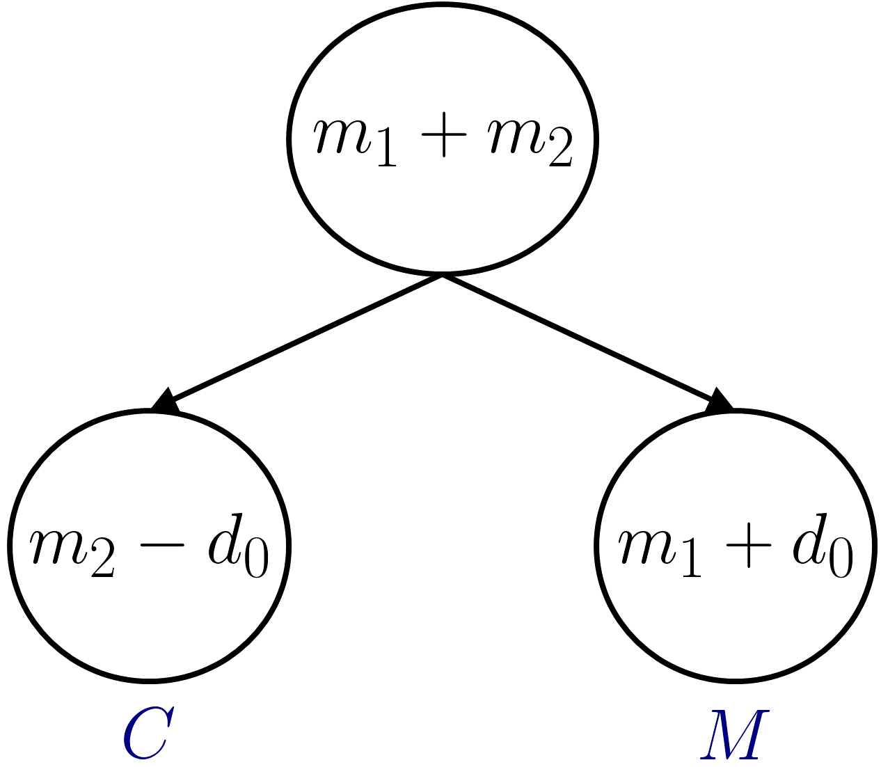
Let and denote the mortality and censoring/survival nodes respectively. For ease of calculation, we estimate the cumulative hazard of the nodes at their respective maximum event times. Let be the maximum event time at node then is given as:
Let , then can be represented as:
| (7) |
Equation 7 can alternately be written as harmonic series as follows:
The sum of the series, with elements can be approximated using the following:
Where, is the Euler-Mascheroni constant (Lagarias, 2013) and is the diagmma function (Abramowitz et al., 1972). Similarly, and so forth. Hence, the hazard estimate for the mortality node can be given as:
| (8) | |||||
Similarly the hazard function for the censoring node, estimated at or after the maximum event time, considering the minimum censoring time to be greater than the maximum event time, can be represented as:
It can be shown that the hazard estimate or survival function of the terminal nodes and thus the RSF is consistent (Ishwaran and Kogalur, 2010). As already defined, denote the true cumulative hazard function with being the density estimate of true survival times , i.e., . Then for a possible infinite time such that the hazard estimate at is finite, using the consistency of Kaplan-Meir estimator, we have,
with convergence rate . However, let us consider a class imbalance with . Then, mortality samples have hazard and the remaining samples have a small hazard of the censored node . However, under any reasonable split (i.e. any censored node has more censored samples than mortality samples and vice versa for the hazard node). The overall estimate of the hazard for mortality samples is and is thus underestimated.
Now, with additional synthetic mortality samples and the new mortality class size , the hazard of the mortality class at becomes:
Also, . Clearly, hazard estimate of the individuals in the mortality node has now improved. Further, the mortality samples present in censored node still have hazard . Nonetheless, the proportion, , thus overall hazard of the individuals in the unbalanced, small size mortality class is underestimated. The underestimation is worsened when the size itself is small. Similarly, when with an additional death samples in the censoring node, the unbalanced hazard is overestimated. The hazard estimate of the censored node with can now be represented as:
| (9) |
Since , , i.e., the hazard for the censored node improves after balancing.
Figure 10, presents the survival probability plots for the veteran, mgus, cost, and lung datasets for which censored class is the minority (pbc dataset has mortality as a minority, refer to Table 1 in the main text). In this figure, the “red curve” represents survival probability of the mortality samples and the “blue curve” represents the survival of the censored samples at different event times. Ideally, the survival probability (approximately opposite of hazard) of the mortality should be low and that for the censored samples should be high. However, due to imbalance, there are several samples which are misclassified. After balancing, the blue curve has shifted upwards (hazard decreased). Further class separation has drastically improved.

Proposition 2 Considering , let and be the surviving and the mortality class size, and the Brier score (BS) before and after balancing respectively. can be approximated as:
where is the maximum number of unique death samples present in the leaf nodes.
Proof. Survival function calculated at a time for the mortality node , and the censored node, are given as follows:
The prediction error of the nodes are then defined in terms of the expected Brier score (refer to subsection 2.2.2) are given as:
where, is the actual survival status of individual at time and is the predicted survival. Further, the predicted survival for individual is the survival estimator for its leaf node. Given the best survival node split as defined above, BS score calculated for the unbalanced data, and can be represented as:
Now, let us again consider and after balancing, let the class proportion be (with fixed and ), the balanced Brier Score can then be given as:
Hence the ratio of and can be represented as:
| (10) |
Corollary 1
Let be the Brier scores before and after balancing the class sizes, then .
Proof. Since , we know that . Now, let , showing that is a decreasing function of would suffice to prove Corollary 1. We perform first order differentiation by parts of with respect to which results in:
| (11) |
Here, and . Further, is the Trigamma function (Abramowitz and Stegun, 1965) which is positive for non-negative number. Clearly, with exponential and Trigamma function being positive, . Now that we have established is a decreasing function, for , the right hand side of Equation 10 becomes less than 1 and hence .
This implies that the prediction of RSF improves after balancing. For similar result holds.
References
- Abramowitz and Stegun (1965) Milton Abramowitz and Irene A Stegun. Handbook of mathematical functions with formulas, graphs, and mathematical table, volume 2172. Dover New York, 1965.
- Abramowitz et al. (1972) Milton Abramowitz, Irene A Stegun, et al. Handbook of mathematical functions with formulas, graphs, and mathematical tables, volume 9. Dover, New York, 1972.
- Amsterdam et al. (2014) Ezra A Amsterdam, Nanette K Wenger, Ralph G Brindis, Donald E Casey, Theodore G Ganiats, David R Holmes, Allan S Jaffe, Hani Jneid, Rosemary F Kelly, Michael C Kontos, et al. 2014 aha/acc guideline for the management of patients with non-st-elevation acute coronary syndromes: executive summary. Circulation, pages CIR–0000000000000133, 2014.
- Belle et al. (2011) Vanya Van Belle, Kristiaan Pelckmans, Johan AK Suykens, and Sabine Van Huffel. Learning transformation models for ranking and survival analysis. Journal of machine learning research, 12(Mar):819–862, 2011.
- Binder (1992) David A Binder. Fitting cox’s proportional hazards models from survey data. Biometrika, pages 139–147, 1992.
- Borgan (2005) Ørnulf Borgan. Nelson–aalen estimator. Encyclopedia of Biostatistics, 2005.
- Breiman (2001) Leo Breiman. Random forests. Machine learning, 45(1):5–32, 2001.
- Breiman et al. (1984) Leo Breiman, Jerome Friedman, Charles J Stone, and Richard A Olshen. Classification and regression trees. CRC press, 1984.
- Cai (1998) Zongwu Cai. Asymptotic properties of kaplan-meier estimator for censored dependent data. Statistics & probability letters, 37(4):381–389, 1998.
- Chawla et al. (2002) Nitesh V Chawla, Kevin W Bowyer, Lawrence O Hall, and W Philip Kegelmeyer. Smote: synthetic minority over-sampling technique. Journal of artificial intelligence research, 16:321–357, 2002.
- Chen et al. (2004) Chao Chen, Andy Liaw, and Leo Breiman. Using random forest to learn imbalanced data. University of California, Berkeley, 110, 2004.
- Chia et al. (2012) Chih-Chun Chia, Ilan Rubinfeld, Benjamin M Scirica, Sean McMillan, Hitinder S Gurm, and Zeeshan Syed. Looking beyond historical patient outcomes to improve clinical models. Science translational medicine, 4(131):131ra49–131ra49, 2012.
- Croal et al. (2006) Bernard L Croal, Graham S Hillis, Patrick H Gibson, Mohammed T Fazal, Hussein El-Shafei, George Gibson, Robert R Jeffrey, Keith G Buchan, Douglas West, and Brian H Cuthbertson. Relationship between postoperative cardiac troponin i levels and outcome of cardiac surgery. Circulation, 114(14):1468–1475, 2006.
- Dankner et al. (2003) Rachel Dankner, Uri Goldbourt, Valentina Boyko, Henrietta Reicher-Reiss, BIP Study Group, et al. Predictors of cardiac and noncardiac mortality among 14,697 patients with coronary heart disease. The American journal of cardiology, 91(2):121–127, 2003.
- Ehrlinger (2016) John Ehrlinger. ggrandomforests: Exploring random forest survival. arXiv preprint arXiv:1612.08974, 2016.
- Friedman et al. (2001) Jerome Friedman, Trevor Hastie, and Robert Tibshirani. The elements of statistical learning, volume 1. Springer series in statistics New York, 2001.
- Furnary et al. (1996) Anthony P Furnary, Juan-Carlos Chachques, Luiz FP Moreira, Gary L Grunkemeier, Jeffrey S Swanson, Noedir Stolf, Sam Haydar, Christoph Acar, Albert Starr, Adib D Jatene, et al. Long-term outcome, survival analysis, and risk stratification of dynamic cardiomyoplasty. The Journal of thoracic and cardiovascular surgery, 112(6):1640–1650, 1996.
- Gerds and Schumacher (2006) Thomas A Gerds and Martin Schumacher. Consistent estimation of the expected brier score in general survival models with right-censored event times. Biometrical Journal, 48(6):1029–1040, 2006.
- Gerds and Schumacher (2007) Thomas A Gerds and Martin Schumacher. Efron-type measures of prediction error for survival analysis. Biometrics, 63(4):1283–1287, 2007.
- Harrell et al. (1982) Frank E Harrell, Robert M Califf, David B Pryor, Kerry L Lee, and Robert A Rosati. Evaluating the yield of medical tests. Jama, 247(18):2543–2546, 1982.
- Harrell Jr (2015) Frank E Harrell Jr. Cox proportional hazards regression model. In Regression modeling strategies, pages 475–519. Springer, 2015.
- Hsich et al. (2011) Eileen Hsich, Eiran Z Gorodeski, Eugene H Blackstone, Hemant Ishwaran, and Michael S Lauer. Identifying important risk factors for survival in patient with systolic heart failure using random survival forests. Circulation: Cardiovascular Quality and Outcomes, 4(1):39–45, 2011.
- Ishwaran and Kogalur (2007) Hemant Ishwaran and Udaya B Kogalur. Random survival forests for r. New Functions for Multivariate Analysis, page 25, 2007.
- Ishwaran and Kogalur (2010) Hemant Ishwaran and Udaya B Kogalur. Consistency of random survival forests. Statistics & probability letters, 80(13):1056–1064, 2010.
- Ishwaran et al. (2008) Hemant Ishwaran, Udaya B Kogalur, Eugene H Blackstone, and Michael S Lauer. Random survival forests. The annals of applied statistics, pages 841–860, 2008.
- Ishwaran et al. (2010) Hemant Ishwaran, Udaya B Kogalur, Eiran Z Gorodeski, Andy J Minn, and Michael S Lauer. High-dimensional variable selection for survival data. Journal of the American Statistical Association, 105(489):205–217, 2010.
- Ishwaran et al. (2011) Hemant Ishwaran, Udaya B Kogalur, Xi Chen, and Andy J Minn. Random survival forests for high-dimensional data. Statistical Analysis and Data Mining: The ASA Data Science Journal, 4(1):115–132, 2011.
- James et al. (2013) Gareth James, Daniela Witten, Trevor Hastie, and Robert Tibshirani. An introduction to statistical learning, volume 112. Springer, 2013.
- Japkowicz (2000) Nathalie Japkowicz. The class imbalance problem: Significance and strategies. In Proc. of the Int’l Conf. on Artificial Intelligence, 2000.
- Japkowicz and Stephen (2002) Nathalie Japkowicz and Shaju Stephen. The class imbalance problem: A systematic study. Intelligent data analysis, 6(5):429–449, 2002.
- Jørgensen et al. (1996) Henrik Stig Jørgensen, Hirofumi Nakayama, Jakob Reith, Hans Otto Raaschou, and Tom Skyhøj Olsen. Acute stroke with atrial fibrillation. Stroke, 27(10):1765–1769, 1996.
- Kalbfleisch and Prentice (2011) John D Kalbfleisch and Ross L Prentice. The statistical analysis of failure time data, volume 360. John Wiley & Sons, 2011.
- Kyle (1993) Robert A Kyle. “benign” monoclonal gammopathy—after 20 to 35 years of follow-up. In Mayo Clinic Proceedings, volume 68, pages 26–36. Elsevier, 1993.
- Lagarias (2013) Jeffrey Lagarias. Euler’s constant: Euler’s work and modern developments. Bulletin of the American Mathematical Society, 50(4):527–628, 2013.
- Loprinzi et al. (1994) Charles Lawrence Loprinzi, John A Laurie, H Sam Wieand, James E Krook, Paul J Novotny, John W Kugler, Joan Bartel, Marlys Law, Marilyn Bateman, and Nancy E Klatt. Prospective evaluation of prognostic variables from patient-completed questionnaires. north central cancer treatment group. Journal of Clinical Oncology, 12(3):601–607, 1994.
- Mogensen et al. (2012) Ulla B Mogensen, Hemant Ishwaran, and Thomas A Gerds. Evaluating random forests for survival analysis using prediction error curves. Journal of statistical software, 50(11):1, 2012.
- O’Gara et al. (2013) Patrick T O’Gara, Frederick G Kushner, Deborah D Ascheim, Donald E Casey, Mina K Chung, James A De Lemos, Steven M Ettinger, James C Fang, Francis M Fesmire, Barry A Franklin, et al. 2013 accf/aha guideline for the management of st-elevation myocardial infarction. Journal of the American College of Cardiology, 61(4):e78–e140, 2013.
- Ohno-Machado (1997) Lucila Ohno-Machado. A comparison of cox proportional hazards and artificial neural network models for medical prognosis. Computers in biology and medicine, 27(1):55–65, 1997.
- Ottani et al. (2000) Filippo Ottani, Marcello Galvani, Francesca Antonia Nicolini, Donatella Ferrini, Andrea Pozzati, Giuseppe Di Pasquale, and Allan S Jaffe. Elevated cardiac troponin levels predict the risk of adverse outcome in patients with acute coronary syndromes. American heart journal, 140(6):917–927, 2000.
- Pan and Schaubel (2008) Qing Pan and Douglas E Schaubel. Proportional hazards models based on biased samples and estimated selection probabilities. Canadian Journal of Statistics, 36(1):111–127, 2008.
- Sawant et al. (2013) Abhishek C Sawant, Swapna R Narra, Paul K Mills, and Sanjay Srivatsa. Prognostic value of frontal qrs-t angle in predicting survival after primary percutaneous coronary revascularisation/coronary artery bypass grafting for stemi. Journal of the American College of Cardiology, 61(10):E97, 2013.
- Segal (1988) Mark Robert Segal. Regression trees for censored data. Biometrics, pages 35–47, 1988.
- Snedecor and Cochran (1989) GW Snedecor and WG Cochran. Statistical methods. ames: Iowa stat, 1989.