A Color-Locus Method for Mapping Using Ensembles of Stars
Abstract
We present a simple but effective technique for measuring angular variation in across the sky. We divide stars from the Pan-STARRS1 catalog into Healpix pixels and determine the posterior distribution of reddening and for each pixel using two independent Monte Carlo methods. We find the two methods to be self-consistent in the limits where they are expected to perform similarly. We also find some agreement with high-precision photometric studies of in Perseus and Ophiuchus, as well as with a map of reddening near the Galactic plane based on stellar spectra from APOGEE. While current studies of are mostly limited to isolated clouds, we have developed a systematic method for comparing values for the majority of observable dust. This is a proof of concept for a more rigorous Galactic reddening map.
I. Introduction
Interstellar dust is an important part of the Milky Way. It is deeply intertwined with the formation and evolution of stars and plays a critical role in the physical and chemical processes of the interstellar medium (ISM). It is also one of the principal foregrounds for other objects of interest within and beyond the Milky Way. Understanding dust and variations in its optical properties will be crucial steps toward understanding the structure of the Galaxy and for making accurate photometric corrections.
The composition of dust, however, remains mostly a mystery. For the better part of a century we have known that there must be a population of fine particles in our Galaxy in order to account for the selective absorption and scattering of bluer wavelengths in observed spectra [42]. Whittet [49] and others showed that the extinction curve of dust varies significantly along different sightlines through the Galaxy. Fitzpatrick & Massa [5] and two subsequent papers by the same authors demonstrated that most extinction curves can be described by analytic expressions with as few as four parameters along typical lines of sight. Cardelli et al. [1, hereafter CCM] then showed that the parameters are largely correlated and thus proposed that the main component of variation in extinction curves can be characterized by a single parameter . is a prudent choice of parameter because is directly related to the slope of the extinction, which is the most salient differentiating feature for the optical and infrared wavelengths. There continues to be debate over whether captures all the significant reddening information for typical extinction curves. For example, Fitzpatrick [4] and Valencic et al. [46] have further refined the single-parameter reddening law first proposed by CCM. On the other hand, Mathis & Cardelli [27] and more recently Fitzpatrick & Massa [6] have shown that one parameter may not be enough to reasonably describe all curves, especially as one ventures further into the ultraviolet or infrared. This suggests that we should avoid assuming any specific class of reddening laws and instead measure the actual per-wavelength reddening as empirically as possible.
So far, many groups have obtained different estimates of reddening in various regions of the sky using different techniques, and it is unclear how comparable these are. New, large surveys like Pan-STARRS1 offer the opportunity to resolve these difficulties, by providing homogeneous photometry across a majority of the sky. This motivates us to develop a technique to determine from photometry alone, allowing extinction curve measurements to be put on a common scale over most of the sky. There have been several studies that use similar techniques. NICE, NICER [19], and NICEST [18] used photometry from the near-IR bands to estimate the total extinction along lines of sight. High et al. [15] and Schlafly et al. [32] used the visual bands to make similar estimates. Our study is different from the above examples in that we estimate the variation in the reddening in addition to the total extinction.
In order to make a full-sky map of reddening, we must have a population of well-characterized sources distributed throughout the whole sky for which we know the intrinsic spectrum. We can then compare the observed spectra to the same model intrinsic spectrum and estimate the selective attenuation - or reddening - of the sources. We must also have some means of evaluating the veracity of a map since there is no other full-sky map of reddening variation currently in existence.
The PS1 catalog provides us with stars that satisfy these criteria. Although a single star measured in the five PS1 bands is not suitable for the pair method (unless the intrinsic colors of that star are known from some other technique, e.g., spectroscopy), a set of stars expected to be reddened by the same dust column has a well-understood locus in color-color space. We introduce two statistical methods for estimating reddening using ensembles of stars along different lines of sight. Stars are divided into Healpix pixels, with each pixel corresponding to a line of sight. The two methods were independently developed, allowing us to check for consistency.
The first method, which henceforth we refer to as the locus-shift method, makes the simplifying assumption that the majority of stars along a line of sight are behind the same dust column. This allows us to fit for the color excess of the entire locus of stars in a pixel, instead of fitting star by star. In the limit that this simple model is accurate, we gain a high signal-to-noise ratio of the position of the locus in color space with a greatly reduced computation time.
The second method uses the Bayestar package [11]. Given a set of stars in a pixel (i.e. a line of sight) and a model of stellar magnitudes based on their luminosity and metallicity, as well as priors on these parameters, Bayestar computes the full posterior of the possible realizations of dust reddening as a function of distance along the line of sight. While the publicly released map in Green et al. [12] has fixed to , in this study we let float. We expect this to provide the most precise map of reddening; however, it requires long computation times, and although we can use Schlegel et al. [37, hereafter SFD] to verify that it has measured extinction reliably, we have no way to determine its accuracy in estimating . By comparing the locus-shift map with the Bayestar map, we can estimate some degree of confidence for each pixel in our maps.
In Section II we describe the data used to generate our maps. We explain the locus-shift method in Section III, describing the locus model in Section III.2, and showing how we convert our reddening estimates to a single parameter in Section III.3. In particular, we discuss the nuances of using a map of as a map of reddening, as well as the dangers of assuming that a simple reddening law holds in all cases. In Section IV we discuss some of the insights into the locus-shift method gained from mock stars, and in Section V we present our locus-shift reddening maps. We then explain how we adapted Bayestar as an alternate method for measuring in Section VI. In Section VII we analyze our locus-shift results and compare them to those from Bayestar, as well as those from the independent study Schlafly et al. [36, hereafter S16]. Finally, in Section VIII we make concluding remarks.
II. Pan-STARRS1
This study uses stellar photometry from approximately million stars from the PS1 survey. The PS1 survey [2] uses a wide-field telescope installed on the peak of Haleakala in Hawaii [16]. An array of pixel CCDs is situated in the focal plane, and the system can swap between the , , , , , and photometric filters [16, 29, 40]. A tunable laser was used to measure the filter transmission functions [38]. The PS1 collaboration provides total expected transmission functions that account for the optical properties of the telescope. We use these to derive the attenuation in the PS1 bands as a function of reddening.
The survey itself covered the entire sky northward of declination , and the PS1 pipeline [20, 26, 25, 47] generated a catalog of most sources in this region brighter than roughly mag, depending on the band and data release [21, 24, 22, 23]. The observations have been further calibrated and characterized by Tonry et al. [41] and Schlafly et al. [34]. We note that as the source detection algorithms improve, new iterations of the reduced data set have been released to the collaboration as Processing Versions [7]. This paper uses the latest Processing Version (PV3). In Sections III and VI, we discuss our criteria for making a selection on this data set.


In the top panel, which we take directly from Green et al. [11], we show the position of a source in color space superposed with a curve following our model for the main-sequence stellar locus. We move the source, purportedly a main-sequence star, backward in the opposite direction of the reddening vector until it intersects with the stellar locus at two possible photometric parallax solutions ( and ). In this manner we can estimate the reddening of a star.
In the bottom panel we repurpose Green’s figure to show our model for the stellar locus (colored line) superposed with the set of stars along a line of sight (black circles). Assuming that all the stars are behind one cloud, we can model their positions in color space with a new reddened locus (gray line). We note that the locus-shift model does not include the bend at the blue end of the locus because it is fit to the observed distribution of stellar colors and does not incorporate information about stellar ages.
III. The Reddening Law via the Locus-shift Method
We estimate the reddening in each pixel using a two-step process that fits an entire locus of stars simultaneously. For the first step, the locus shift, we take an unreddened locus model and fit for the shifts in color-color space that best approximate the position of the observed locus of stars from each pixel. Since PS1 has magnitudes in five bands and four possible informative colors, this is a four-parameter fit. For the second step, the reddening fit, we find the most likely and based on the locus shifts. Since estimates of can be very different for different reddening laws, the results are only intended to be used to reveal very general properties of the ISM. We strongly encourage detailed comparisons to be made not with our values, but with the underlying color excesses.
We have organized the subsections as follows. In Section III.1 we establish the general framework for the first step of our analysis, the locus shift. We provide a top-level description of our method for fitting shifts in color space and then proceed to lay out the details of the theory behind the method. Next, in Section III.2, we describe our procedure for empirically generating the most important component of our method, the locus model. We explain the limits of the model, then provide the technical details, and finally argue for the cuts used to generate the model. In Section III.3 we go over the second step of our analysis, the reddening fit. We show three different methods for converting locus-shift color excesses to reddenings (i.e. two numbers and ). Finally, in Section III.4 we reiterate the importance of considering all dependencies when choosing a reddening model, and we argue for the particular choices made in this paper.
III.1. Estimating Locus Shifts in Color Space
Please see the bottom panel of Figure 1 for a schematic drawing of the locus fits described below. The locus-shift method has the advantage of being able to estimate the reddening of each color by combining information for multiple stars. The locus-shift method works best when there is a single predominant and relatively nearby source of reddening for a line of sight. In such a case most of the stars in the pixel are shifted in color space by the same reddening vector, resulting in the entire unreddened locus being shifted to its observed reddened position in color space. Fortunately, this situation is common for nearby dust clouds situated off the Galactic plane. In this limit we expect our results to agree well with other independent measurements of , as well as the alternate Bayestar method we outline later in Section VI.
More rigorously, let and be the magnitudes and colors, respectively, of the star in a Healpix pixel. We choose to subtract adjacent bands to obtain our colors, so that all color vectors are in the color space. The empirically determined unreddened locus , i.e. the average stellar locus expected for lines of sight with no dust, is described by a curve through color-color space, , as well as a distribution along the locus . We find the color to be a reasonable choice for the parameter , in that and can both be accurately described by low-order polynomials. We explain the derivation of the locus in detail in Section III.2.1. Given some color excess , we get the reddened locus
| (1) |
Since this is akin to moving the unreddened locus model in color space, in the context of our Monte Carlo model we will call the locus shift and conceptually separate it from the color excess of a single source.
Figure 2 shows an example of a locus-shift fit. The black line corresponds to the unreddened locus , and the red line is the reddened locus after being displaced by . As expected, is centered among the stellar colors for this pixel.
For some position on the locus, the probability of a star’s colors is given by a modified normal distribution in color excess
| (2) | |||||
| (3) |
where is the covariance matrix derived from the uncertainties in stellar colors. If we let be the element of corresponding to the colors and , and if we let be the covariance between band magnitudes and , then given the basis of colors and the basis of magnitudes , we get the relation
| (4) |
as demonstrated in Green et al. [11]. We choose so that is a function that asymptotically approaches for offsets less than and flattens out to a constant value when the total offset is beyond . These wings in the distribution allow us to reject outlier stars that deviate from the locus as a result of either not being on the main sequence or having drastically different reddening from the other stars in the pixel. Marginalizing over the locus, the likelihood for the colors of all the stars in a pixel is then
| (5) |
Note that we have absorbed the variation in metallicity into the systematics and account for any corresponding uncertainties when we calculate . We take the standard deviations of the residuals of each color from our model fits and add these to the diagonals of . This of course accounts for any systematic, but we expect metallicity to be the largest component. The uncertainties are , , , and for , , , and , respectively.
We fit for using a Metropolis–Hastings Monte Carlo to sample from the posterior
| (6) |
We generally use a flat prior . This allows us to apply empirically determined priors on later on in our analysis.
We save samples from each Monte Carlo chain of originally samples. We discard the first saved samples as burn-in whenever we calculate any statistics. Each pixel has three chains with different initial conditions, giving us samples total. To test for convergence, we use a Gelman–Rubin diagnostic.
We note that this technique is similar to stellar locus regression, which High et al. [15] showed to be effective for making corrections for atmospheric and dust extinction when estimating the photometric redshifts of galaxies.
III.2. The Locus Model
Our stellar locus models are all derived empirically by fitting the colors of stars from regions of low dust emission in Schlegel et al. [37]. This ensures that our fits are accurate in the low-dust limit, as we are not dependent on a theoretical model of the mass function and metallicity distribution that reconstructs observed stellar colors. However, our reliance on empirical stellar loci makes it challenging to know how accurate our stellar locus is in the Galactic plane, where no low reddening regions are available. Moreover, low-latitude stars are more likely to be younger and more metal rich than typical high-latitude halo stars, leading us to expect our stellar locus to poorly represent stars directly in the Galactic plane. We discuss ways to resolve this in Section V.1 and also provide a mask to avoid problematic regions, as detailed throughout Section V
III.2.1 Empirical Stellar Loci
In order to make an accurate empirical model, we need a set of real stars completely unobscured by dust. However, since this is impossible, we correct the colors of stars by assuming a reddening law and using SFD [37] as a template for dust optical depth. The locus model is then a best-fit curve to the unreddened stellar colors for a set of stars in regions with an effective :
| (7) |
We use the Fitzpatrick [4] reddening law with set to , as that has been found to be describe the mean reddening at low dust columns [32]. Assuming that our locus model is correct, our choice of reddening law for this dereddening procedure has little effect on our locus-shift fits to real data for pixels with . Pixels with low dust do experience a bias, but since these regions inherently have little reddening information, they are masked in our results.
Figure 3 shows an example unreddened locus model. It is a five-dimensional function of a single variable, the color . Four of the dimensions describe the curve traced out by the mean locus through the space comprising the colors , , , and . The fifth dimension is the density of stars in . The density effectively serves as a luminosity function, and we marginalize over this distribution when finding the likelihood of a star’s colors. itself is a dummy variable for relating the five dimensions to one another, and it has no bearing on the result of the integral in the likelihood function in Equation 5.
III.2.2 Cuts for Generating the Locus Model
To obtain the best loci for carrying out fits, we exclude stars that are not likely to be on the main sequence, as well as those with bad photometry. For the first case, we cut stars that lie blueward of our unreddened locus models. Since dust extinction can only move stars along the reddening vector in color-color space, any detection beyond the blue end of our locus is most likely a white dwarf or a quasar. We keep detections redder than our unreddened locus since obviously these are likely to be real stars obscured by dust. Stars that pass these cuts but are not in reality main-sequence stars should be effectively ignored in our fits owing to the wings in the probability distribution described in Eq. 2. For the second case, we cut stars that are fainter than mag in the band, which excludes stars with low signal-to-noise ratios.
III.3. Estimating the Reddening Law
Once we have a chain of locus shifts for each pixel, we find the and that best approximate the distribution of . This effectively entails a projection from the four-dimensional color space down into a two-dimensional reddening law subspace. We employ a few different methods depending on the comparison we wish to make. By decoupling from the Monte Carlo locus fits, we can quickly iterate over different reddening laws and save computation time for more accurate locus shifts. This lets us be flexible with the extinction models we use, instead of presupposing a specific reddening law. Since there have not been many comprehensive studies of variation, we believe that this is crucial for extracting the most accurate and useful information from our fits.
However, there are some dangers in arbitrarily converting locus shifts to for comparison with other data sets, especially when other photometric surveys may include different sets of stars and different passbands, so we recommend using the locus shifts in our data product as much as possible. If the reader still finds it necessary to obtain some value, we describe below three different methods for estimating reddenings and list their pros and cons, both to provide the reader with options and to inform them of the types of pitfalls we encountered. We suggest the proxy defined below because it is most closely tied to the canonical definition of , but we emphasize that the link between and is model dependent. For especially noisy data, the reader may be better served by the first method listed below, a gradient descent fit to a reddening law of choice, since it uses information from all four color shifts. Furthermore, we recommend extra precaution when converting between different formulations of , as demonstrated in Figure 4
III.3.1 Gradient Descent
When we wish to determine the expected for a specific reddening law, we use a gradient descent algorithm with a chi-square goodness of fit.
Let be a reddening law function that returns a set of color shifts, given the parameters and reddening (this is the same numerically integrated function defined by Equation 18). The likelihood of a color shift is then
| (8) |
where is a multivariate normal function with mean and covariance matrix evaluated at . is calculated directly from the distribution of samples in the locus-shift Monte Carlo chains.
The posterior is
| (9) |
We find that the distribution of samples in parameter space is roughly Gaussian. Therefore, we find it faster and sufficient to use a gradient descent search to determine the most likely .
We fit a number of reddening laws to the locus shifts in order to find the most accurate one. For the objective function, we use the mean of all pixels with since in this regime the fits should neither be sensitive to our choice of locus model nor to the unique reddening properties found in dense clouds. For CCM, O’Donnell [28], and Fitzpatrick [4, hereafter F99], we get reduced values of , , and , respectively. Therefore, we use F99 to generate the unreddened locus models above. However, the consistently high values show that none of the standard reddening models capture the full variability in reddening in the Milky Way.
A more principled method would be to convert the samples to samples using a function that maps to . Although this does not address the need for more than one reddening parameter, it allows us to examine the distribution of the posterior in . In the next section we demonstrate how to make a linear projection that is a good approximation of such a mapping function.
III.3.2 Linear Transforms
Since our fit results are coordinates in color space, and since the two-dimensional manifold mapped by and through color space has very little curvature regardless of the reddening law we choose, we are able to linearize the conversion from locus shift to a coordinate in some affine subspace, i.e. , for some projection , without much loss of information. In fact, for some function given by a reddening law like F99, for example, , we can reproduce the relation to within a few hundredths of using only a second-order polynomial of .
This property of and in principle allows us to compare values derived by the locus-shift method with those derived using principal components in 36. It also allows us to quickly calculate a distribution of . By taking the first principal component to be the true mean reddening vector for the Milky Way, we can express as and get as a function of the ratio of . Unfortunately, it turns out that the mean reddening vector given in 36 and the one derived by this study using PS1 stars are not the same. We have identified three main contributing factors. First, the 36 study uses three Two Micron All Sky Survey bands and two WISE bands in addition to the five PS1 bands used here. This means that vectors that are orthogonal in the 10-band space will no longer be so in the five-band space. Our different conventions for linearizing the reddening vector necessitate this. This is largely not an issue because we can simply project one linearization to the other, and indeed doing so shows that they span roughly the same planes.
The second factor, which is related to the first, is the result of both studies being insensitive to any gray components in the reddening vector. This means that we must fit to a reasonable reddening law in order to obtain color ratios. Doing this fit, with five bands or bands, produces different mean reddening vectors. The 3D subspaces spanned by , , and for both studies show even closer agreement with each other than the subspaces spanned by just and . However, we cannot simply force them to agree by fitting to to each other since both vectors are degenerate with the distance modulus and thus potentially encode real physical properties of the stars.
The third factor is that the APOGEE survey focused on giants, whereas PS1 only has a photometric limit, implying that most sources will be main-sequence stars. This means that, given some detection limit, the two surveys include stars at different distances and behind different dust columns. Additionally, stars with different spectra have different integrated fluxes through bandpasses and thus have different reddening vectors for the same extinction curve. By comparing sightlines with high evidence of having only one predominant source of reddening, we can mitigate the former effect, but in general we expect the mean reddening vector to be different.
On the other hand, these effects are irrelevant when applying two different analyses to the same data set. Therefore, we use a principal component formulation of when comparing our locus-shift results with Bayestar results in Section VII.2. Projecting the 36 principal components to be orthogonal in the PS1 bands, we get the vectors presented in the table below.
We convert the linear transformations to reddening parameters via the formulae
| (10) | |||
| (11) |
which have been adapted from 36 and fit to F99.
In summary, this means that our locus-shift samples are linearizable when comparing values derived from band magnitudes from similar wavelength ranges and similar sets of sources. However, when extrapolating to different wavelengths or using different sources, we must be careful to make the correct linear projection and to use a self-consistent definition of . We suggest a method for addressing these issues in the next section.


For both panels we generate some locus shifts assuming that F99 is the true reddening in a dust cloud. Then we convert the locus shifts back to using a proxy and compare with the original according to F99. In the top panel we use the proxy , which is the formula we get if we substitute for W2 in Equation 13 using the relations given by , the mean reddening vector in 36. In the bottom panel we use Equation 12, whose constants have been obtained by fitting the proxy to F99 directly. As expected, the latter agrees more closely with F99 since we have optimized the constants to do so. The discrepancy in the top panel is not due to errors in either our models or those used in 36, but rather is the result of fitting the function to a model other than F99, i.e. , which itself was accurate for the data in 36. In other words, although the F99 and 36 extinction curves have similar behavior over a broad range of wavelengths, extrapolating them from a narrow range can lead to very different results.
We therefore recommend using the full locus-shift fits when making comparisons and only converting to when evaluating specific reddening laws such as F99.
III.3.3 An Proxy
We are inclined to formulate a definition of that is as insensitive as possible to the above effects. The best solution would be to use a model of reddening that incorporates stellar types and dust extinction for a given set of photometric bands, and this will be the topic of future papers. In the meantime we adopt Equations 12 for reddenings from PS1 and Equation 13 for reddenings from 36. We choose them for some useful properties listed below, but note that there are many other reasonable formulations as well, especially due to the variability of the reddening vector:
| (12) |
| (13) |
These definitions have the advantage of both being mathematically similar to the original formulation in that behaves similarly to and and are similar to for the sources involved. Equation 13, as well as the strategy of using this functional form, was taken from 36. Equation 13 works specifically because 36 matched data for sources from the PS1 and WISE surveys, allowing them to correlate reddenings in the PS1 , , and WISE 2 bands, and fit the relation to F99. As long as the user is careful to use the correct linear coefficients, biases from selection effects should be minimized. See Figure 4 for details.
We also note that Equations 12 and 13 agree with each other for a wide range of values and typical reddenings because they have been fit to an independent empirical estimate of the typical reddening in the Galaxy (namely, F99). To be more precise, in as much as the true locus shift for a pixel lies at a point in color space close to the F99 color surface, both formulae will agree with each other and serve as excellent proxies for the canonical definition of . Most other empirically derived reddening laws, such as CCM, lie somewhat close to F99 in color space, but not enough for perfect agreement. This is especially true for the mean reddening vector provided by 36, and so we elect to tie our parameterization to F99 via Equation 12 when comparing to results from the principal component analysis in 36.
We hope this further illustrates the need to use all the information in a locus shift or color excess when making reddening comparisons, rather than projecting down into space.
III.4. Choosing an Extinction Model
To summarize, our reddening estimates first involve using a Metropolis–Hastings sampler to obtain the posterior distribution of locus shifts in color space. Next, we convert the locus shifts to a reddening parameter according to some extinction model. We have described three different ways to make this conversion: a gradient descent fit to a reddening law, linearizing the color-excess information into reddening vectors, or calculating via a proxy formula tied to a model for the reddening in different bands. For the range of wavelengths in the PS1 survey, all of these models are relatively linear, and for the majority of pixels covered by the survey, our locus-shift results tend to be very similar, or can be converted to one another with a simple linear transformation. Since we are looking for correlations between our estimated values and those of other studies, in the context of this paper our results are robust for any choice of the three conversion methods.
For all the plots in Section V and onward we use the proxy definition of from Equation 12 (even though it does not affect our conclusions), since it is similar to the definition used in 36 and because its physical motivation is straightforward. This formula is tied to F99 because, as shown in Section III.3.1, F99 has the lowest of the standard reddening laws when fit to our locus-shift results. To estimate , we fit F99 to the locus shifts via gradient descent, as per Section III.3.1. The one exception to the above is where we use the principal component model from Section III.3.2 when comparing locus-shift fits to Bayestar fits owing to the latter having a natural linear formulation. If the reader needs to use some definition of to make their own comparison, they should carefully consider the pros and cons of each method listed above.
IV. Mock Stars
We test the reliability of the locus-shift method by running our analysis on a set of mock stars. We simulate the effects of dust on stellar colors in order to better understand how our model fits should behave in various situations. The colors of stars are simulated by using the locus models as follows:
- 1.
For each star, a point is chosen along the locus curve in color space.
- 2.
The probability density of choosing a coordinate is specified by the distribution.
- 3.
The color coordinates are displaced by a random color vector with a normal distribution. This accounts for the uncertainty in color measurements, as well as systematic uncertainties from ignoring metallicity.
- 4.
Next, the colors are shifted according to the reddening vectors corresponding to the dust column in front of each star.
- 5.
Colors for a single star may be shifted several times to simulate multiple dust clouds with different reddening.
The resulting set of reddened stellar colors allow us to test for a variety of cases. We generate mock stars for the following scenarios:
- 1.
All the stars are behind a single dust cloud. We simply shift all stellar colors in a pixel by the same reddening vector for this case.
- 2.
A fraction of the stars in a pixel have a different amount of reddening compared to others in the same pixel. We expect this to occur when the dust column has spatial variation at subpixel angular scales, e.g. in dense cores and filaments.
- 3.
A fraction of the stars in a pixel are reddened by one more cloud in addition to a nearby cloud that reddens all the stars in the pixel. This corresponds to the case where there are multiple layers of clouds along a line of sight.
Sanity checks of the Bayestar method can be found in Green et al. [11] and Green et al. [12]


IV.1. Mock Scenario: A Single Cloud
Figures 5 and 6 show how the residuals look for a single cloud - i.e. a discrete sudden increase in reddening - along a line of sight. This corresponds to the simple model used in the locus-shift method and thus should yield the smallest residuals. The stellar colors have been generated for a range of and values for the mock dust cloud, and in the plots we show the marginalized distribution of residuals for each of the reddening parameters. There is a slight bias introduced by a selection effect where redder stars and stars behind dust with lower are cut before other stars owing to the band dropping below threshold. This causes the estimated extinction to be grayer and results in a positive residual. Nevertheless, with these mock runs we are able to reproduce the ’true’ to within , which is much less than the typical uncertainty of in our posteriors. We determine to within , an order of magnitude less than the uncertainties in our posteriors.
IV.2. Mock Scenario: Subpixel Variation
In Figure 7 we show how our fits respond to a pixel with subpixel variation in dust column density. For this scenario we have two populations of stars, one behind dust with a column density corresponding to and another behind dust with . We generate stellar colors for a range of values and also let the fraction of stars in the latter population vary from to . We plot the marginalized distribution of residuals as a function of . The majority of residuals are less than , once again less than the uncertainty in our posteriors. This is an intentionally pathological test case. Most pixels have smoother variation in extinction, even in the densest cores.
IV.3. Mock Scenario: Multiple Cloud Layers
More typical pixels have low subpixel spatial variation in extinction and instead have stars interspersed among dust clouds at multiple distances along a line of sight. This means that some stars in a pixel have additional reddening owing to being behind more clouds. We generate stellar colors for this scenario by first reddening half the stars in a pixel with a fixed reddening vector of and and then reddening all the stars (including the half already reddened) with an additional reddening vector of varying and . This models the effect of one nearby cloud of varying reddening being in front of all stars in a pixel and an additional cloud of fixed reddening appearing at the median distance of the stars. In these situations, residuals in are typically around when we compare the estimated of the entire pixel to the simulated values for the closer cloud. Figure 8 shows the marginalized distribution of residuals as a function of the true of the closer cloud. We obtain the ’correct’ answer for the closer cloud owing to selection bias. Stars behind extra dust are more likely to be cut or not observed owing to increased extinction. Additionally, those that do pass the cut are fainter than stars behind only the first cloud, and we expect the former to have less influence on our fits. Figure 9 makes the same comparison as a function of the true of the closer cloud.
Altogether, we see that our fits should be accurate to in for most lines of sight where the reddenings are well approximated by a single dust cloud. They are also expected to be accurate to in even in some problematic lines of sight.

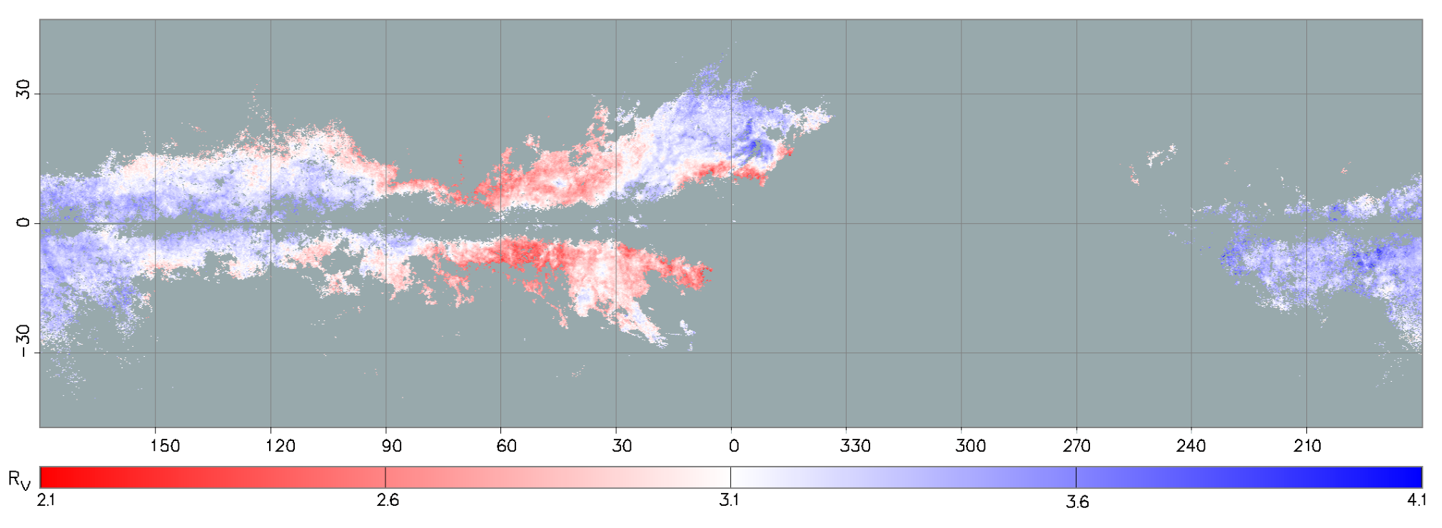
V. The Locus-shift Map
In Figure 10 we present maps of and , converted from locus shifts as specified in Section III.4. We also zoom in on interesting clouds in Figures 11–14. The maps are at and run from to . In the map, white corresponds to greater extinction, and the cool gray denotes pixels with no information. For the map, white corresponds to , red is for values less than , and blue is for values greater than . We select pixels that are above a threshold in both and a quality factor related to the reliability of a pixel (as defined below). The threshold ensures that we are insensitive to unmodeled variations in the stellar population, and the threshold ensures that the fits themselves are informative. On the other hand, for the zoomed-in maps we employ a value mask so that darker values correspond to less reliable pixels, with black denoting no available information. We choose the hard cut for the large map to make it easier to see the smoothly varying spatial trends in through the Galaxy. We choose the value mask for the zoomed-in maps to convey more information about pixel uncertainties. We also hope that these two different graphical representations demonstrate to the reader that the maps are only intended to give rough ideas of variations, and that for detailed comparisons it is best to use the full reddening vectors provided in our data release, along the related uncertainties.
V.1. Accounting for Galactic Variation with the Threshold
Since stellar populations vary across the Galaxy, we must have a method for estimating or accounting for their effects on our fits. Following the process outlined in Section III.2.1, we construct a model locus for low galatic latitudes and another for high latitudes. This dual model assumes that stellar populations can be modeled by a thick disk and a halo component, and that all lines of sight of interest are some combination of these two. Since our targets avoid regions with high extinction (see Section V), we do not need to model the thin disk or the bulge. We run our fits with both models and find that the two sets of results begin to agree with each other within uncertainties when the total extinction . We claim that the thick disk and halo models represent the maximum possible variation in the stellar locus, and thus use to select pixels we do not expected to be dominated by model uncertainties.
We note that the threshold of is greater than the value of required to be insensitive to variations in the unreddened locus because differences in colors for different stellar populations are greater than those introduced by the de-reddening procedure. We therefore use the larger value for all analyses below, unless otherwise stated. Furthermore, given that we are using the proxy definition (from Section III.3.3), the threshold allows us to avoid biases that may arise from having a small value of in the denominator.
V.1.1 Accounting for Fitting Uncertainties with the Quality Factor
The reliability of a pixel is based on a quality factor that depends on the evidence per star and the uncertainty in , defined as follows:
| (14) |
where is the evidence, is the number of stars, and the constant is chosen so that and have roughly the same standard deviation as each other for a pixel well-described by our locus-shift model. We find to be a reasonable choice, but note that this number is flexible. For example, if we were to use a different parameterization for , a different value of may be optimal. Although we recommend a cut at for rough comparisons, the best method for estimating confidence in a fit would be to determine whether the evidence or standard deviation (or some other statistic of the posterior) is most relevant for the particular use case. The formula above has been optimized primarily for visual inspection of reddening maps. For plotting purposes, we convert to
| (15) |
which has a more even distribution from to and is intuitively similar to the evidence multiplied by a probability related to the uncertainty in . This makes well suited for masking out Healpix pixels based on our confidence in the fit parameters.
As expected, masks out regions with few stars or low reddening, since there is not enough information for a good fit. It also masks out regions with a lot of continuous reddening along the line of sight (instead of discrete clouds) because the stars in the pixel have been attenuated by too wide a range of reddening vectors, and the locus-shift model is a bad approximation of the data. Such cases occur predominantly around the Galactic plane.
V.2. Accessing the Map
The locus-shift map can be downloaded as a FITS file from the Harvard Dataverse via the link http://dx.doi.org/10.7910/DVN/TJGJWW. The structure of the data is as described in Table 1:
| Key (Tag) | Format | Description |
|---|---|---|
| healpix | int64 | (Healpix, ) |
| nstars | int64 | no. of stars |
| locus_shift_mean | float64 | mean locus-shift (LS) |
| locus_shift_best | float64 | best LS |
| covariance | float64 | covariances of LS |
| logZ | float64 | log of evidence |
| Gelman_Rubin | float64 | GR diagnostic of LS |
| RV_EBV_F99 | float64 | (, , , ) |
| RV_EBV_PC | float64 | (, , , ) |
| RV_proxy | float64 | (, ) |
| Qfactor | float64 | (, , ) |
In the table, is shorthand for . Every element or row in the first data unit has the ten keys listed above. Each element corresponds to a Healpix pixel for which we have data. The content of each key is summarized above. locus_shift_mean and locus_shift_best are -element double precision arrays of the mean locus-shift and the best locus-shift sample, respectively. The elements correspond to the , , , and color-shifts. covariance is the full covariance matrix of color-shifts. RV_EBV_F99 has four elements corresponding to the mean , mean , standard deviation of , and standard deviation of of the locus-shifts according to the F99 reddening law. RV_EBV_PC has the same structure, except according to the principal component formulation (Eq. 10). RV_proxy reports just the and its standard deviation according to the proxy formula from Section III.3.3. Finally, Qfactor gives the quality factor , a masking fraction (Eq. 15), and an adjusted masking fraction
| (16) |
where is roughly , a sigmoid function centered on the threshold . We use as a value mask in the plots in Figures 11–14.
| Target | locus-shift | literature | reference | |
|---|---|---|---|---|
| Perseus | – | – | [8] | |
| Oph core | – | ∗ | [3] | |
| Oph cloud | – | Whittet [48] | ||
| Alessi 95 | [45] | |||
| Pleiades | [43] | |||
| NGC 1647 | ||||
| Messier 4 | [14] | |||
| Collinder 394 | [44] |
As evidenced by comparing the two panels, is highly correlated with in this cloud, which corroborates some theories about grain size distributions in dense clouds. On the other hand, the correlation may just imply that our parameters have artificial dependencies. Figure 12 proves that this is not the case, and that we are independently sensitive to both and .
Additionally, the lack of correlation in Cepheus may have been due to changing stellar populations as we move closer to the galactic disk, but the next two Figures 13 and 14 show that exhibits behavior contrary to this as well.
V.3. for Nearby Dust Clouds
We compare our results with other studies that measure along a specific line of sight. In Table 2 we make our best effort to include all available papers as of this writing which (a) give results for a specific location or locations in the sky and (b) are covered by the PS1 footprint. There are several tens of papers such as Gontcharov [9] and Sung & Bessell [39] which provide spatial variations of but are not constrained enough to allow comparison with our results. After selecting for studies that overlap with the region of sky covered by PS1, we have a handful of targets. We find a broad range of estimated values from cloud to cloud, and although the numbers do not agree exactly, we find that the variation in our estimates are positively correlated with those from previous studies.
We also find some features of note in select clouds. E.g. we sometimes see a positive correlation between and in clouds such as Ophiuchus (Figure 11 ) but do not see them in areas like the clouds in Cepheus (Figure 12). If we had seen the former property consistently throughout the sky, it may have been due to artificial correlations in our model parameters. However, regions like Cepheus show very little correlation between and , and Perseus and Orion even exhibit the opposite correlation, albeit very subtly (Figures 13 and 14). The different types of correlations show that our analysis is measuring a real reddening effect, and that it is potentially sensitive to complex properties of dust. The correlation in Ophiuchus itself may be due to its being at a stage of formation where its pressure and radiation field are conducive to large grain formation. We see a similar, but less pronounced, correlation between the dust column and in the densest cores of Taurus and Perseus.
The dust in Cepheus also seems to consist of two distinct populations. Dust above degrees in galactic latitude has relatively low , whereas the portion at has elevated . The separation along corroborates the spatial structure of the Cepheus Flare described in Schlafly et al. [35] as well as Grenier et al. [13] and Kun et al. [17], providing further evidence that the Flare is two clouds along coincident lines of sight.
VI. The Reddening Law via Bayestar
Bayestar is a C++ package for performing Bayesian analysis on stellar photometry to determine the reddenings to and stellar types of a set of stars. It was developed by Gregory Green to produce a 3D map of dust in the Milky Way [12]. Please refer to Green et al. [11] and Green et al. [12] for a complete overview of the techniques used by Bayestar. The following paragraphs describe a rather specific and limited application of Bayestar for the purpose of inferring .
In the context of this study, we use Bayestar to test the efficacy of fitting for per-star stellar posteriors in order to estimate the reddening from dust along a line of sight. If one dust cloud along a line of sight that accounts for the majority of reddening, we expect the reddening estimate given by Bayestar to be close to that given by the locus-shift method. Since this use case is easy to understand, we attempt to show that Bayestar is a well-behaved and reliable estimator of reddening for such lines of sight. This should provide a foundation for future studies that will use better data and models. For example, when Gaia data are released, we will be able to use distance constraints to more accurately estimate stellar type and reddening.
We note that in comparison to the locus-shift method, Bayestar assumes that the space of all possible reddenings (i.e. shifts in color space) is two-dimensional, and does not have the flexibility to explore arbitrary reddening laws. If all reddenings in the Milky Way do indeed lie in a two-dimensional space, then Bayestar naturally provides a better model for any reddening or selection effect that may arise owing to complex dust distributions and stellar populations along a line of sight. By comparing the two methods, we can corroborate one against the other, as well as determine the most efficient method for estimating reddening.
Our strategy with Bayestar is to fit for the stellar type (parameterized by ), metallicity , distance modulus , , and of a star given its magnitudes. The model developed in Green et al. [11] uses a function of and to get the intrinsic colors of a star and then adds the expected attenuation from , , and to get the full model magnitude:
| (17) |
We have abbreviated as the variable since the model does not treat it as a function of passbands, but rather as a parameter for specifying the dust column density to a star. is the reddening vector, which denotes the displacement in magnitude space due to dust extinction. The function itself is derived by integrating for each of the PS1 bands the expected reduction in flux from a typical main-sequence star due to dust:
| (18) |
is the band throughput provided by Tonry et al. [41], is the spectrum for a typical star, and is the throughput of photons at due to some quantity and type of dust specified by and . That is, is determined by the extinction curve, which we define according to a reddening law such as F99. We then combine for all bands to obtain . A detailed treatment is available in the appendix of Schlafly & Finkbeiner [31]. The likelihood is then
| (19) |
where is a multivariate normal with mean and standard deviations . Given some priors on the parameters, we can then obtain the posterior for a star. The posteriors for some stars with large uncertainties tend to either be multimodal or have an extremely elongated non-Gaussian shape, due to the surfaces mapped out by the locus model in parameter space. Please see the top panel of Figure 1 for a graphical representation of the model and a visual explanation of how it differs from the locus-shift model.
We caution the reader that the model in this section assumes a specific reddening law. We use a principal component formulation that has been fit to F99 owing to evidence in favor of its being an accurate model for the PS1 bands [31]. However, this means that the reddening vectors probed by our Monte Carlo sampler only lie on a subsurface within the space of all possible extinctions. If some dust cloud were to have a reddening not well described by F99, then our fit for would not be reliable.
VI.1. Method for Estimating with Bayestar
Our method is as follows: We use a parallel affine-invariant sampler adapted from Goodman & Weare [10] and run chains for each star using the model described above [11]. Stars are selected from the full list of sources based on whether there is detection in at least four bands and whether the point-spread function is point-like (i.e. it is not a galaxy). We use a kernel density estimator to find the marginal posterior as a function of . A grid spacing of and a Gaussian kernel with FWHM times the grid spacing, i.e. , give a resolution equal to the typical uncertainty in for a dust column of approximately .
We then take the product of the posterior distributions of all the stars in a single pixel. Assuming that there must only be a single value for a sufficiently small pixel, this is the joint probability distribution of for all stars in a pixel. In reality we found that a few percent of the sources in a pixel tend to be outliers owing either to bad photometry or to not being a main-sequence star. In order to account for this, we modify each stellar posterior distribution to be a sum of the original marginalized distribution and an additional flat distribution from to that has been normalized to have a total integrated probability times that of the marginalized distribution, i.e., .
The end result is an distribution for every pixel in the sky that contains PS1 sources. We note that since we have marginalized over the distance modulus, this map does not have 3D information like the ones published by the related work Green et al. [11]. This is an intentional simplification for the purposes of drastically decreasing computational time and for making a more direct comparison with the alternate reddening maps in this paper, which are both 2D.
Our distribution of values agrees with most publications in the literature. It is centered around with an FWHM of . There is also no significant correlation with the other fit parameters, except for a slight increase for very high values of , which could be due to the dust grain population. We compare our Bayestar results with our locus-shift method in Section VII. We note that in order to make such a comparison, we require some method for estimating a degree of belief for the reddenings we find on a pixel-by-pixel basis. We use the evidence for this purpose. We provide the details of our method for calculating it in the Appendix.
VII. Discussion
VII.1. The Reddening Law

Among the more widely cited reddening laws, we find F99 to be the best fit to our locus-shift results. Converting our locus shifts to via the proxy in Equation 12, we find the mean to be with an FWHM of (Figure 15). This is in agreement with the distribution found by S16. As described in Section III.4, we fit F99 to the locus shifts via gradient descent in order to obtain the corresponding values. We find that there are three populations of pixels roughly divided at values of and and lying above or below the median line (Figure 16). It is not yet clear at the present level of analysis whether this is a by-product of having an incomplete model or the result of varying properties in different populations of dust. Pixels lying above the median line tend to be closer to the direction of the Galactic anticenter, whereas pixels in the two populations below the line tend to be closer to the Galactic center and exhibit a bimodal distribution in and space. In the current data product there is too much spatial mixing for us to conclude that this is a real physical feature.
In general, increases slightly for larger column densities but is mostly independent of , as demonstrated by our detailed examination of Ophiuchus and Cepheus, as well as the distribution shown in Figure 16. However, there are localized correlations, and in particular, some dense cloud cores exhibit highly elevated values. This effect exceeds any variations in our mock catalogs (see Section IV), and we have reason to believe that it is real since other studies have found similar properties in dust clouds. A frequently cited reason for this correlation is that the higher concentrations of dust grains in dense clouds may facilitate the formation of larger grains, which in turn shield against UV radiation that may destroy dust mantles. The larger grain population results in a shallower extinction curve in the visible wavelengths owing to Rayleigh and Mie scattering.
We also note that, although mostly masked out by our recommended quality factor threshold, pixels near the Galactic plane tend to have elevated , except for those near the bulge, which have low . These are regions where our model is not a good descriptor of the data, due to both varying stellar populations and multiple layers of dust. In fact, the systematic offset may be caused by our fits being sensitive to such differences in the properties of the stars and dust. This may suggest an opportunity to extract even more information from PS1 photometry given more sophisticated models.
VII.2. Bayestar versus Locus Shift
We find agreement between our results for the Bayestar method and the locus-shift method. In Figure 17 we plot values from Bayestar against those from the locus-shift method. Each point is an comparison for a Healpix pixel. Although individual clouds do not show a strong correlation, the coarse spatial variation of across the whole sky is consistent from cloud to cloud. Since the two methods are largely independent, we have some confidence that we are estimating real variations in the reddening law.
In order to make this comparison, we have to convert from locus shifts to a definition of close to what is modeled by Bayestar’s reddening law. In order to facilitate this, we parameterize Bayestar’s allowed reddenings according to the space mapped by the first two principal reddening components from 36. This covers a subspace in color space that is very similar to that mapped by F99 but has the additional advantage of being linear. This in turn allows us to convert locus shifts into corresponding values using simple linear transformations, as described in Section III.3.2.
The above procedure makes our two derivations of consistent. However, the output of the locus-shift method after the conversion to is a single chain of values for each pixel. On the other hand, the output of our Bayestar method is a chain of values for every single star in each pixel. Therefore, we take the product of the distributions of all the stars in each pixel (see Section VI.1).
The main discrepancies between the two methods in Figure 17, i.e. the slope and the offset in the mean values, can probably be attributed to the fact that - despite our best efforts as described above - it is impossible to equate the two results since the respective Monte Carlo chains project the probabilities associated with a pixel into different subspaces. To be more precise, Bayestar projects reddening information into the subspace of extinctions mapped by F99 first before fitting for individual stellar likelihoods and subsequently calculating the likelihood of all stars in a pixel, whereas the locus-shift method evaluates the combined likelihood of all the stars in a pixel while fitting for the full reddening distribution in color space. Therefore, Bayestar is losing reddening information, while the locus-shift method is losing information from individual stars. Furthermore, the slope of the relation is fairly sensitive to our choice of priors for either method, and although we keep all shared priors identical for our analysis, there are unique priors for which we must ultimately provide a best guess based on other literature (e.g. priors for metallicity or the full reddening vector). With this context, it is perhaps more assuring that we have a significantly positive correlation at all.
VII.3. PS1 versus APOGEE


We expect the reddening maps from 36 to be reliable not only because they are empirically determined from photometry, like our locus-shift map, but also because the stellar types of the sources were fit independently of the dust reddenings to the sources. This was made possible by the detailed temperature information made available by the APOGEE survey. By tying the stellar type fits to the temperature, one can decouple reddening from stellar types and obtain better constraints on . In this regard we expect comparisons with 36 to be the strongest tests currently available of the reliability of the locus-shift and Bayestar methods. This of course will change when more Gaia data are released.
We find to be correlated for the different surveys and methods. We find a positive correlation between the results from 36 and the values from both our Bayestar and locus-shift methods (Figure 18). Although the slope between the Bayestar and S16 results shows a correlation not as strong as that between locus-shift and S16, both comparisons clearly demonstrate that all three surveys are sensitive to the same reddening information.
We also corroborate the negative correlation between and Planck that was discovered by S16. In Figure 19 we show the – relationship from our results. The location and shape of the distribution are strikingly similar to those in Figure 18 of S16. We also find that this relationship persists independently of cuts on latitude or dust column.
We additionally find to be consistent between different PS1 processing versions (Figure 20), which shows that our estimates of reddening are robust even under different reductions of the PS1 surveys.
VIII. Conclusion
Historically it has been difficult to measure reddenings reliably over the entire sky owing to the lack of a consistent data set with sufficient coverage. We present one of the first maps of reddening variation in the Milky Way for a majority of the sky. This is the first reddening map based purely on PS1 photometry, as well as the first to cover more than half of the sky at a -arcminute resolution. Comparisons of our locus-shift results with other reddening measurements show that careful modeling of the photometry of typical stars allows us to obtain mutually consistent estimates of the spatial variation in dust reddening. We publish the map as a set of Healpix pixels, providing both the full reddening vectors (i.e. locus shifts) and the converted values.
Upon inspection of the maps, we observe the following:
- 1.
The Bayestar and locus-shift methods obtain estimates of that are reasonably correlated, despite using very different models and algorithms.
- 2.
Mock data show the locus-shift method to be self-consistent in the limits where it is expected to agree with Bayestar.
- 3.
We find the distribution and spatial variation in the reddening maps to be consistent with Fitzpatrick [4] and Schlafly et al. [36], respectively.
- 4.
We find further agreement with several detailed studies of in a set of well-characterized nearby dust clouds.
Given the level of self-consistency, as well as agreement with other studies, we believe that our algorithms are probing the actual reddenings of stars. We have demonstrated that Bayestar and the locus-shift method reliably estimate in all the limiting cases we can easily check. In particular, with the right models and data, even a simple locus-regression algorithm can be an effective tool for quickly estimating the reddening law. We expect the locus-shift method to be a useful sanity check when making a full 3D map of reddening with Bayestar, and we aim to extend Bayestar so that it can be sensitive to all dimensions of reddening along a line of sight. We should be able to corroborate future results from Bayestar with 3D studies like Schlafly et al. [33], as well as surveys with better distance information such as Gaia. Altogether, we have shown that it is possible to use large photometric surveys to make multiple independent estimates of reddening across the Milky Way.
VIII.1. Acknowledgments
A.L. acknowledges support for this research provided by the NSF. This material is based on work supported by the National Science Foundation Graduate Research Fellowship under grant no. DGE 1144152. This work is also supported by NSF grants AST-1312891 and AST-1614941. E.S. acknowledges support for this work provided by NASA through Hubble Fellowship grant HST-HF2-51367.001-A awarded by the Space Telescope Science Institute, which is operated by the Association of Universities for Research in Astronomy, Inc., for NASA, under contract NAS 5-26555.
We would like to thank the Pan-STARRS1 collaboration for providing us with high-quality photometry for millions of stars across of the sky. The Pan-STARRS1 Surveys (PS1) and the PS1 public science archive have been made possible through contributions by the Institute for Astronomy, the University of Hawaii, the Pan-STARRS Project Office, the Max-Planck Society and its participating institutes, the Max Planck Institute for Astronomy, Heidelberg, and the Max Planck Institute for Extraterrestrial Physics, Garching, The Johns Hopkins University, Durham University, the University of Edinburgh, the Queen’s University Belfast, the Harvard-Smithsonian Center for Astrophysics, the Las Cumbres Observatory Global Telescope Network Incorporated, the National Central University of Taiwan, the Space Telescope Science Institute, the National Aeronautics and Space Administration under grant no. NNX08AR22G issued through the Planetary Science Division of the NASA Science Mission Directorate, the National Science Foundation grant no. AST-1238877, the University of Maryland, Eotvos Lorand University (ELTE), the Los Alamos National Laboratory, and the Gordon and Betty Moore Foundation.
The analyses presented in this paper were run on the Odyssey cluster at Harvard University. We would like to acknowledge the staff at the FAS Research Computing Group, who not only manage the Odyssey cluster but also provide maintenance on our own dedicated machines.
We thank Mario Juric for building the Large Survey Database framework, which powers all the queries made to our local copy of the PS1 data set.
This research has made use of NASA’s Astrophysics Data System Bibliographic Services.
Finally, we appreciate the many useful comments from Aaron Meisner, Stephen Portillo, Tansu Daylan, Catherine Zucker, Ioana Zelko, Blakesley Burkhart, Zachary Slepian, Ana Bonaca, Josh Speagle, Ben Lee, Karin Oberg, and Vinothan Manoharan.
References
- [1] Cardelli, J. A., Clayton, G. C., & Mathis, J. S. 1989, ApJ, 345, 245
- [2] Chambers, K. C., Magnier, E. A., Metcalfe, N., et al. 2016, ArXiv e-prints, arXiv:1612.05560
- [3] Chapman, N. L., Mundy, L. G., Lai, S.-P., & Evans, II, N. J. 2009, ApJ, 690, 496
- [4] Fitzpatrick, E. L. 1999, PASP, 111, 63
- [5] Fitzpatrick, E. L., & Massa, D. 1986, ApJ, 307, 286
- [6] —. 2009, ApJ, 699, 1209
- [7] Flewelling, H. A., Magnier, E. A., Chambers, K. C., et al. 2016, ArXiv e-prints, arXiv:1612.05243
- [8] Foster, J. B., Mandel, K. S., Pineda, J. E., et al. 2013, MNRAS, 428, 1606
- [9] Gontcharov, G. A. 2013, Astronomy Letters, 39, 550
- [10] Goodman, J., & Weare, J. 2010, CAMCOS, 5, 65
- [11] Green, G. M., Schlafly, E. F., Finkbeiner, D. P., et al. 2014, ApJ, 783, 114
- [12] —. 2015, ApJ, 810, 25
- [13] Grenier, I. A., Lebrun, F., Arnaud, M., Dame, T. M., & Thaddeus, P. 1989, ApJ, 347, 231
- [14] Hendricks, B., Stetson, P. B., VandenBerg, D. A., & Dall’Ora, M. 2012, AJ, 144, 25
- [15] High, F. W., Stubbs, C. W., Rest, A., Stalder, B., & Challis, P. 2009, AJ, 138, 110
- [16] Hodapp, K. W., Kaiser, N., Aussel, H., et al. 2004, AN, 325, 636
- [17] Kun, M., Kiss, Z. T., & Balog, Z. 2008, in Handbook of Star Forming Regions: Vol. I, ed. B. Reipurth (San Francisco, CA: ASP), 136
- [18] Lombardi, M. 2009, A&A, 493, 735
- [19] Lombardi, M., & Alves, J. 2001, A&A, 377, 1023
- [20] Magnier, E. 2006, in The Advanced Maui Optical and Space Surveillance Technologies Conference, ed. S. Ryan (Kihei, HI: The Maui Economic Developer Board), E50
- [21] Magnier, E. 2007, in Astronomical Society of the Pacific Conference Series, Vol. 364, The Future of Photometric, Spectrophotometric and Polarimetric Standardization, ed. C. Sterken, 153–+
- [22] Magnier, E. A., Liu, M., Monet, D. G., & Chambers, K. C. 2008, in IAU Symposium, Vol. 248, IAU Symp. 248, A Giant Step: from Milli- to Micro-arcsecond Astrometry, ed. W. J. Jin, I. Platais, & M. A. C. Perryman (Cambridge: Cambridge Univ. Press), 553–559
- [23] Magnier, E. A., Schlafly, E., Finkbeiner, D., et al. 2013, ApJS, 205, 20
- [24] Magnier, E. A., Schlafly, E. F., Finkbeiner, D. P., et al. 2016a, ArXiv e-prints, arXiv:1612.05242
- [25] Magnier, E. A., Sweeney, W. E., Chambers, K. C., et al. 2016b, ArXiv e-prints, arXiv:1612.05244
- [26] Magnier, E. A., Chambers, K. C., Flewelling, H. A., et al. 2016c, ArXiv e-prints, arXiv:1612.05240
- [27] Mathis, J. S., & Cardelli, J. A. 1992, ApJ, 398, 610
- [28] O’Donnell, J. E. 1994, ApJ, 422, 158
- [29] Onaka, P., Tonry, J. L., Isani, S., et al. 2008, in Society of Photo-Optical Instrumentation Engineers (SPIE) Conference Series, Vol. 7014, Society of Photo-Optical Instrumentation Engineers (SPIE) Conference Series, 70140D
- [30] Robert, C. P., & Wraith, D. 2009, in American Institute of Physics Conference Series, Vol. 1193, Bayesian Inference and Maximum Entropy Methods in Science and Engineering: The 29th International Workshop on Bayesian Inference and Maximum Entropy Methods in Science and Engineering, ed. P. M. Goggans & C.-Y. Chan (Melville, NY: AIP), 251–262
- [31] Schlafly, E. F., & Finkbeiner, D. P. 2011, ApJ, 737, 103
- [32] Schlafly, E. F., Finkbeiner, D. P., Schlegel, D. J., et al. 2010, ApJ, 725, 1175
- [33] Schlafly, E. F., Peek, J. E. G., Finkbeiner, D. P., & Green, G. M. 2017, ApJ, 838, 36
- [34] Schlafly, E. F., Finkbeiner, D. P., Jurić, M., et al. 2012, ApJ, 756, 158
- [35] Schlafly, E. F., Green, G., Finkbeiner, D. P., et al. 2014, ApJ, 786, 29
- [36] Schlafly, E. F., Meisner, A. M., Stutz, A. M., et al. 2016, ApJ, 821, 78
- [37] Schlegel, D. J., Finkbeiner, D. P., & Davis, M. 1998, ApJ, 500, 525
- [38] Stubbs, C. W., Doherty, P., Cramer, C., et al. 2010, ApJS, 191, 376
- [39] Sung, H., & Bessell, M. S. 2014, in Astronomical Society of the Pacific Conference Series, Vol. 482, Tenth Pacific Rim Conference on Stellar Astrophysics, ed. H.-W. Lee, Y. W. Kang, & K.-C. Leung, 275–277
- [40] Tonry, J., & Onaka, P. 2009, in Advanced Maui Optical and Space Surveillance Technologies Conference, ed. S. Ryan (Kihei, HI: The Maui Economic Developer Board), E40
- [41] Tonry, J. L., Stubbs, C. W., Lykke, K. R., et al. 2012, ApJ, 750, 99
- [42] Trumpler, R. J. 1930, PASP, 42, 214
- [43] Turner, D. G. 1976, AJ, 81, 1125
- [44] Turner, D. G., & Pedreros, M. 1985, AJ, 90, 1231
- [45] Turner, D. G., Majaess, D. J., Lane, D. J., et al. 2012, MNRAS, 422, 2501
- [46] Valencic, L. A., Clayton, G. C., & Gordon, K. D. 2004, ApJ, 616, 912
- [47] Waters, C. Z., Magnier, E. A., Price, P. A., et al. 2016, ArXiv e-prints, arXiv:1612.05245
- [48] Whittet, D. C. B. 1974, MNRAS, 168, 371
- [49] —. 1977, MNRAS, 180, 29
Appendix A Harmonic Mean Estimation of the Evidence
The harmonic mean estimator allows us to calculate the evidence of some data by only using the likelihoods and priors of samples in a chain. Starting with a simple relation for the Bayesian evidence , we can derive the expression as follows:
| (20) | |||||
| (21) | |||||
| (22) | |||||
| (23) | |||||
| (24) | |||||
| (25) |
In Equation 22, the regulating function is an arbitrary normalized function. If the factor is well behaved over the entire domain of , then we can bring it inside the integral since by definition it should be a constant. After some rearranging, we get an expectation of samples drawn from the posterior . In practice, we can use the relation 25 to estimate the evidence as long as the regulating function falls to zero faster than the posterior [30].
Because the distribution of the posterior in space is highly irregular, we must be careful about picking a valid regulating function. We opt to use a constant four-dimensional ellipsoid that is zero outside its boundaries and centered at the highest likelihood sample from the Monte Carlo chains. This ensures that there are a high number of samples in that region of parameter space and that the posterior will be well behaved in the immediate vicinity. Making the boundary of be a step function ensures that it falls off faster than the posterior, and it makes it easy to normalize. Since the shape of the posterior can vary drastically in different parts of parameter space, we recalculate the local covariance matrix of samples near the regulating region so that we can update the principal axes of the ellipsoid to better approximate the posterior.
Since we do not let the Monte Carlo chains have negative reddening, the prior is effectively for . Thus, we must make sure not to include this region in our regulating function. We achieve this by requiring the ellipsoid center to be at least some distance from , and if necessary, we renormalize the regulating function after ignoring the fraction of its volume in negative .
The accuracy of the harmonic estimator is primarily limited by Poisson statistics since we are effectively counting the number of samples that fall inside the regulating ellipsoid. This requires us to run longer chains since generally only of samples fall inside the ellipsoid. Of course, in pixels with a large number of stars we get a reduction in this noise when determining the total probability of the pixel:
| (26) |
We find steps to be sufficient for most pixels. To further reduce the noise, we use multiple regulating ellipsoids for each chain. We choose the location of each ellipsoid iteratively: we pick the highest-likelihood sample as the center of the first ellipsoid, then we pick the next-highest-likelihood sample that is outside some small exclusion zone around the first ellipsoid, etc. This ensures that the ellipsoids will all be different and all in regions with high sample density.