Context Encoding for Semantic Segmentation

Hang Zhang Kristin Dana Jianping Shi Zhongyue Zhang
Xiaogang Wang Ambrish Tyagi Amit Agrawal Affiliation: ¹Rutgers University ²Amazon Inc ³SenseTime ⁴The Chinese University of Hong Kong Affiliation: {zhang.hang@,kdana@ece.}rutgers.edu, shijianping@sensetime.com Affiliation: xgwang@ee.cuhk.edu.hk, {zhongyue,ambrisht,aaagrawa}@amazon.com

Abstract

Recent work has made significant progress in improving spatial resolution for pixelwise labeling with Fully Convolutional Network (FCN) framework by employing Dilated/Atrous convolution, utilizing multi-scale features and refining boundaries. In this paper, we explore the impact of global contextual information in semantic segmentation by introducing the Context Encoding Module, which captures the semantic context of scenes and selectively highlights class-dependent featuremaps. The proposed Context Encoding Module significantly improves semantic segmentation results with only marginal extra computation cost over FCN. Our approach has achieved new state-of-the-art results 51.7% mIoU on PASCAL-Context, 85.9% mIoU on PASCAL VOC 2012. Our single model achieves a final score of 0.5567 on ADE20K test set, which surpasses the winning entry of COCO-Place Challenge 2017. In addition, we also explore how the Context Encoding Module can improve the feature representation of relatively shallow networks for the image classification on CIFAR-10 dataset. Our 14 layer network has achieved an error rate of $3.45\%$ , which is comparable with state-of-the-art approaches with over $10\times$ more layers. The source code for the complete system are publicly available¹¹ 1 Links can be found at http://hangzh.com/.

1 Introduction

Refer to caption — Figure 1: Labeling a scene with accurate per-pixel labels is a challenge for semantic segmentation algorithms. Even humans find the task challenging. However, narrowing the list of probable categories based on scene context makes labeling much easier. Motivated by this, we introduce the Context Encoding Module which selectively highlights the class-dependent featuremaps and makes the semantic segmentation easier for the network. (Examples from ADE20K [61].)

Semantic segmentation assigns per-pixel predictions of object categories for the given image, which provides a comprehensive scene description including the information of object category, location and shape. State-of-the-art semantic segmentation approaches are typically based on the Fully Convolutional Network (FCN) framework [37]. The adaption of Deep Convolutional Neural Networks (CNNs) [29] benefits from the rich information of object categories and scene semantics learned from diverse set of images [10]. CNNs are able to capture the informative representations with global receptive fields by stacking convolutional layers with non-linearities and downsampling. For conquering the problem of spatial resolution loss associated with downsampling, recent work uses Dilated/Atrous convolution strategy to produce dense predictions from pre-trained networks [4, 54]. However, this strategy also isolates the pixels from the global scene context, leading to misclassified pixels. For example in the 3^rd row of Figure 4, the baseline approach classifies some pixels in the windowpane as door.

Recent methods have achieved state-of-the-art performance by enlarging the receptive field using multi-resolution pyramid-based representations. For example, PSPNet adopts Spatial Pyramid Pooling that pools the featuremaps into different sizes and concatenates them the after upsampling [59] and Deeplab proposes an Atrous Spatial Pyramid Pooling that employs large rate dilated/atrous convolutions [5]. While these approaches do improve performance, the context representations are not explicit, leading to the questions: Is capturing contextual information the same as increasing the receptive field size? Consider labeling a new image for a large dataset (such as ADE20K [61] containing 150 categories) as shown in Figure 1. Suppose we have a tool allowing the annotator to first select the semantic context of the image, (e.g. a bedroom). Then, the tool could provide a much smaller sublist of relevant categories (e.g. bed, chair, etc.), which would dramatically reduce the search space of possible categories. Similarly, if we can design an approach to fully utilize the strong correlation between scene context and the probabilities of categories, the semantic segmentation becomes easier for the network.

Classic computer vision approaches have the advantage of capturing semantic context of the scene. For a given input image, hand-engineered features are densely extracted using SIFT [38] or filter bank responses [30, 48]. Then a visual vocabulary (dictionary) is often learned and the global feature statistics are described by classic encoders such as Bag-of-Words (BoW) [26, 8, 46, 13], VLAD [25] or Fisher Vector [44]. The classic representations encode global contextual information by capturing feature statistics. While the hand-crafted feature were improved greatly by CNN methods, the overall encoding process of traditional methods was convenient and powerful. Can we leverage the context encoding of classic approaches with the power of deep learning? Recent work has made great progress in generalizing traditional encoders in a CNN framework [1, 58]. Zhang et al. introduces an Encoding Layer that integrates the entire dictionary learning and residual encoding pipeline into a single CNN layer to capture orderless representations. This method has achieved state-of-the-art results on texture classification [58]. In this work, we extend the Encoding Layer to capture global feature statistics for understanding semantic context.

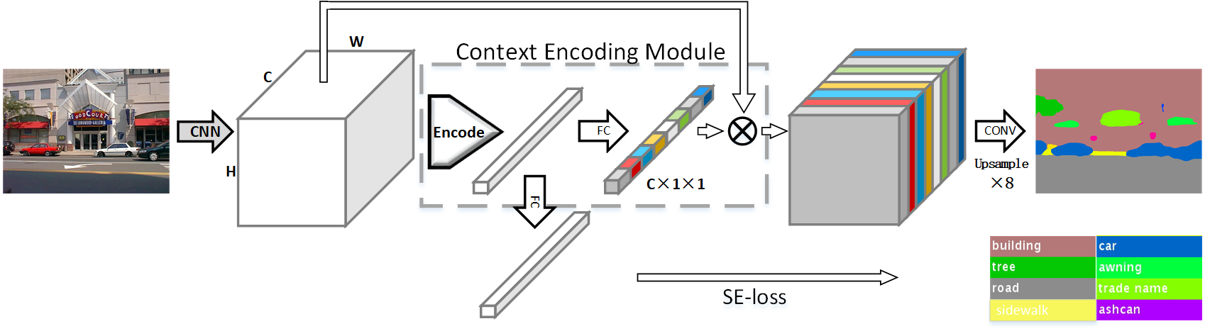
As the first contribution of this paper, we introduce a Context Encoding Module incorporating Semantic Encoding Loss (SE-loss), a simple unit to leverage the global scene context information. The Context Encoding Module integrates an Encoding Layer to capture global context and selectively highlight the class-dependent featuremaps. For intuition, consider that we would want to de-emphasize the probability of a vehicle to appear in an indoor scene. Standard training process only employs per-pixel segmentation loss, which does not strongly utilize global context of the scene. We introduce Semantic Encoding Loss (SE-loss) to regularize the training, which lets the network predict the presence of the object categories in the scene to enforce network learning of semantic context. Unlike per-pixel loss, SE-loss gives an equal contributions for both big and small objects and we find the performance of small objects are often improved in practice. The proposed Context Encoding Module and Semantic Encoding Loss are conceptually straight-forward and compatible with existing FCN based approaches.

The second contribution of this paper is the design and implementation of a new semantic segmentation framework Context Encoding Network (EncNet). EncNet augments a pre-trained Deep Residual Network (ResNet) [17] by including a Context Encoding Module as shown in Figure 2. We use dilation strategy [54, 4] of pre-trained networks. The proposed Context Encoding Network achieves state-of-the-art results 85.9% mIoU on PASCAL VOC 2012 and 51.7% on PASCAL in Context. Our single model of EncNet-101 has achieved a score of 0.5567 which surpass the winning entry of COCO-Place Challenge 2017 [61]. In addition to semantic segmentation, we also study the power of our Context Encoding Module for visual recognition on CIFAR-10 dataset [28] and the performance of shallow network is significantly improved using the proposed Context Encoding Module. Our network has achieved an error rate of $3.96\%$ using only $3.5M$ parameters. We release the complete system including state-of-the-art approaches together with our implementation of synchronized multi-GPU Batch Normalization [23] and memory-efficient Encoding Layer [58].

2 Context Encoding Module

We refer to the new CNN module as Context Encoding Module and the components of the module are illustrated in Figure 2.

Context Encoding

Understanding and utilizing contextual information is very important for semantic segmentation. For a network pre-trained on a diverse set of images [10], the featuremaps encode rich information what objects are in the scene. We employ the Encoding Layer [58] to capture the feature statistics as a global semantic context. We refer to the output of Encoding Layer as encoded semantics. For utilizing the context, a set of scaling factors are predicted to selectively highlight the class-dependent featuremaps. The Encoding Layer learns an inherent dictionary carrying the semantic context of the dataset and outputs the residual encoders with rich contextual information. We briefly describe the prior work of Encoding Layer for completeness.

Encoding Layer considers an input featuremap with the shape of $C\times H\times W$ as a set of $C$ -dimensional input features $X=\{x_{1},...x_{N}\}$ , where $N$ is total number of features given by $H\times W$ , which learns an inherent codebook $D=\{d_{1},...d_{K}\}$ containing $K$ number of codewords (visual centers) and a set of smoothing factor of the visual centers $S=\{s_{1},...s_{K}\}$ . Encoding Layer outputs the residual encoder by aggregating the residuals with soft-assignment weights $e_{k}=\sum_{i=1}^{N}e_{ik}$ , where

e_{ik}=\frac{exp(-s_{k}\|r_{ik}\|^{2})}{\sum_{j=1}^{K}exp(-s_{j}\|r_{ij}\|^{2})}r_{ik},

(1)

and the residuals are given by $r_{ik}=x_{i}-d_{k}$ . We apply aggregation to the encoders instead of concatenation. That is, $e=\sum_{k=1}^{K}\phi(e_{k})$ , where $\phi$ denotes Batch Normalization with ReLU activation, avoid making $K$ independent encoders to be ordered and also reduce the dimensionality of the feature representations.

Featuremap Attention

To make use of the encoded semantics captured by Encoding Layer, we predict scaling factors of featuremaps as a feedback loop to emphasize or de-emphasize class-dependent featuremaps. We use a fully connected layer on top of the Encoding Layer and a sigmoid as the activation function, which outputs predicted featuremap scaling factors $\gamma=\delta(We)$ , where $W$ denotes the layer weights and $\delta$ is the sigmoid function. Then the module output is given by $Y=X\otimes\gamma$ a channel wise multiplication $\otimes$ between input featuremaps $X$ and scaling factor $\gamma$ . This feedback strategy is inspired by prior work in style transfer [57, 22] and a recent work SE-Net [20] that tune featuremap scale or statistics. As an intuitive example of the utility of the approach, consider emphasizing the probability of an airplane in a sky scene, but de-emphasizing that of a vehicle.

Semantic Encoding Loss

In standard training process of semantic segmentation, the network is learned from isolated pixels (per-pixel cross-entropy loss for given input image and ground truth labels). The network may have difficulty understanding context without global information. To regularize the training of Context Encoding Module, we introduce Semantic Encoding Loss (SE-loss) which forces the network to understand the global semantic information with very small extra computation cost. We build an additional fully connected layer with a sigmoid activation function on top of the Encoding Layer to make individual predictions for the presences of object categories in the scene and learn with binary cross entropy loss. Unlike per-pixel loss, SE-loss considers big and small objects equally. In practice, we find the segmentation of small objects are often improved. In summary, the Context Encoding Module shown in Figure 2 captures the semantic context to predict a set of scaling factors that selectively highlights the class-dependent featuremap for semantic segmentation.

2.1 Context Encoding Network (EncNet)

With the proposed Context Encoding Module, we build a Context Encoding Network (EncNet) with pre-trained ResNet [17]. We follow the prior work using dilated network strategy on pre-trained network [6, 59, 55] at stage 3 and 4²² 2 We refer to the stage with original featuremap size 1/16 as stage 3 and size 1/32 as stage 4., as shown in Figure 3. We build our proposed Context Encoding Module on top of convolutional layers right before the final prediction, as shown in Figure 2. For further improving the performance and regularizing the training of Context Encoding Module, we make a separate branch to minimize the SE-loss that takes the encoded semantics as input and predicts the presence of the object classes. As the Context Encoding Module and SE-loss are very light weight, we build another Context Encoding Module on top of stage 3 to minimize the SE-loss as an additional regularization, similar to but much cheaper than the auxiliary loss of PSPNet [59]. The ground truths of SE-loss are directly generated from the ground-truth segmentation mask without any additional annotations.

Our Context Encoding Module is differentiable and inserted in the existing FCN pipeline without any extra training supervision or modification of the framework. In terms of computation, the proposed EncNet only introduces marginal extra computation to the original dilated FCN network.

2.2 Relation to Other Approaches

Segmentation Approaches

CNN has become de facto standard in computer vision tasks including semantic segmentation. The early approaches generate segmentation masks by classifying region proposals [14, 15]. Fully Convolutional Neural Network (FCN) pioneered the era of end-to-end segmentation [37]. However, recovering detailed information from downsampled featuremaps is difficult due to the use of pre-trained networks that are originally designed for image classification. To address this difficulty, one way is to learn the upsampling filters, i.e. fractionally-strided convolution or decoders [3, 41]. The other path is to employ Atrous/Dilated convolution strategy to the network [4, 54] which preserves the large receptive field and produces dense predictions. Prior work adopts dense CRF taking FCN outputs to refine the segmentation boundaries [5, 7], and CRF-RNN achieves end-to-end learning of CRF with FCN [60]. Recent FCN-based work dramatically boosts performance by increasing the receptive field with larger rate atrous convolution or global/pyramid pooling [6, 35, 59]. However, these strategies have to sacrifice the efficiency of the model, for example PSPNet [59] applies convolutions on flat featuremaps after Pyramid Pooling and upsampling and DeepLab [5] employs large rate atrous convolution that will degenerate to $1\times 1$ convolution in extreme cases. We propose the Context Encoding Module to efficiently leverage global context for semantic segmentation, which only requires marginal extra computation costs. In addition, the proposed Context Encoding Module as a simple CNN unit is compatible with all existing FCN-based approaches.

Featuremap Attention and Scaling

The strategy of channel-wise featuremap attention is inspired by some pioneering work. Spatial Transformer Network [24] learns an in-network transformation conditional on the input which provides a spatial attention to the featuremaps without extra supervision. Batch Normalization [23] makes the normalization of the data mean and variance over the mini-batch as part of the network, which successfully allows larger learning rate and makes the network less sensitive to the initialization method. Recent work in style transfer manipulates the featuremap mean and variance [11, 22] or second order statistics to enable in-network style switch [57]. A very recent work SE-Net explores the cross channel information to learn a channel-wise attention and has achieved state-of-the-art performance in image classification [20]. Inspired by these methods, we use encoded semantics to predict scaling factors of featuremap channels, which provides a mechanism to assign saliency by emphasizing or de-emphasizing individual featuremaps conditioned on scene context.

3 Experimental Results

Method	BaseNet	Encoding	SE-loss	MS	pixAcc%	mIoU%
FCN	Res50				73.4	41.0
EncNet	Res50	✓			78.1	47.6
EncNet	Res50	✓	✓		79.4	49.2
EncNet	Res101	✓	✓		80.4	51.7
EncNet	Res101	✓	✓	✓	81.2	52.6

Table 1: Ablation study on PASCAL-Context dataset. Encoding represents Context Encoding Module, SE-loss is the proposed Semantic Segmentation loss, MS means multi-size evaluation. Notably, applying Context Encoding Module only introduce marginal extra computation, but the performance is significantly improved. (PixAcc and mIoU calculated on 59 classes w/o background.)

In this section, we first provide implementation details for EncNet and baseline approach, then we conduct a complete ablation study on Pascal-Context dataset [40], and finally we report the performances on PASCAL VOC 2012 [12] and ADE20K [61] datasets. In addition to semantic segmentation, we also explore how the Context Encoding Module can improve the image classification performance of shallow network on CIFAR-10 dataset in Sec 3.5.

3.1 Implementation Details

Our experiment system including pre-trained models are based on open source toolbox PyTorch [42]. We apply dilation strategy to stage 3 and 42 of the pre-trained networks with the output size of 1 $/$ 8 [4, 54]. The output predictions are upsampled 8 times using bilinear interpolation for calculating the loss [6]. We follow prior work [59, 5] to use the learning rate scheduling $lr=baselr*(1-\frac{iter}{total\_iter})^{power}$ . The base learning rate is set to 0.01 for ADE20K dataset and 0.001 for others and the power is set to 0.9. The momentum is set to 0.9 and weight decay is set to 0.0001. The networks are training for 50 epochs on PASCAL-Context [40] and PASCAL VOC 2012 [12], and 120 epochs on ADE20K [61]. We randomly shuffle the training samples and discard the last mini-batch. For data augmentation, we randomly flip and scale the image between 0.5 to 2 and then randomly rotate the image between -10 to 10 degree and finally crop the image into fix size using zero padding if needed. For evaluation, we average the network prediction in multiple scales following [59, 35, 45].

In practice, larger crop size typically yields better performance for semantic segmentation, but also consumes larger GPU memory which leads to much smaller working batchsize for Batch Normalization [23] and degrades the training. To address this difficulty, we implement Synchronized Cross-GPU Batch Normalization in PyTorch using NVIDIA CUDA & NCCL toolkit, which increases the working batchsize to be global mini-batch size (discussed in Appendix A). We use the mini-batch size of 16 during the training. For comparison with our work, we use dilated ResNet FCN as baseline approaches. For training EncNet, we use the number of codewords 32 in Encoding Layers. The ground truth labels for SE-loss are generated by “unique” operation finding the categories presented in the given ground-truth segmentation mask. The final loss is given by a weighted sum of per-pixel segmentation loss and SE-Loss.

Evaluation Metrics We use standard evaluation metrics of pixel accuracy (pixAcc) and mean Intersection of Union (mIoU). For object segmentation in PASCAL VOC 2012 dataset, we use the official evaluation server that calculates mIoU considering the background as one of the categories. For whole scene parsing datasets PASCAL-Context and ADE20K, we follow the standard competition benchmark [61] to calculate mIoU by ignoring background pixels.

3.2 Results on PASCAL-Context

Method	BaseNet	mIoU%
FCN-8s [37]		37.8
CRF-RNN [60]		39.3
ParseNet [35]		40.4
BoxSup [9]		40.5
HO_CRF [2]		41.3
Piecewise [32]		43.3
VeryDeep [51]		44.5
DeepLab-v2 [5]	Res101-COCO	45.7
RefineNet [31]	Res152	47.3
EncNet (ours)	Res101	51.7

Table 2: Segmentation results on PASCAL-Context dataset. (Note: mIoU on 60 classes w/ background.)

PASCAL-Context dataset [40] provides dense semantic labels for the whole scene, which has 4,998 images for training and 5105 for test. We follow the prior work [40, 5, 31] to use the semantic labels of the most frequent 59 object categories plus background (60 classes in total). We use the pixAcc and mIoU for 59 classes as evaluation metrics in the ablation study of EncNet. For comparing to prior work, we also report the mIoU using 60 classes in Table 2 (considering the background as one of the classes).

Method aero bike bird boat bottle bus car cat chair cow table dog horse mbike person plant sheep sofa train tv mIoU FCN [37] 76.8 34.2 68.9 49.4 60.3 75.3 74.7 77.6 21.4 62.5 46.8 71.8 63.9 76.5 73.9 45.2 72.4 37.4 70.9 55.1 62.2 DeepLabv2 [4] 84.4 54.5 81.5 63.6 65.9 85.1 79.1 83.4 30.7 74.1 59.8 79.0 76.1 83.2 80.8 59.7 82.2 50.4 73.1 63.7 71.6 CRF-RNN [60] 87.5 39.0 79.7 64.2 68.3 87.6 80.8 84.4 30.4 78.2 60.4 80.5 77.8 83.1 80.6 59.5 82.8 47.8 78.3 67.1 72.0 DeconvNet [41] 89.9 39.3 79.7 63.9 68.2 87.4 81.2 86.1 28.5 77.0 62.0 79.0 80.3 83.6 80.2 58.8 83.4 54.3 80.7 65.0 72.5 GCRF [49] 85.2 43.9 83.3 65.2 68.3 89.0 82.7 85.3 31.1 79.5 63.3 80.5 79.3 85.5 81.0 60.5 85.5 52.0 77.3 65.1 73.2 DPN [36] 87.7 59.4 78.4 64.9 70.3 89.3 83.5 86.1 31.7 79.9 62.6 81.9 80.0 83.5 82.3 60.5 83.2 53.4 77.9 65.0 74.1 Piecewise [32] 90.6 37.6 80.0 67.8 74.4 92.0 85.2 86.2 39.1 81.2 58.9 83.8 83.9 84.3 84.8 62.1 83.2 58.2 80.8 72.3 75.3 ResNet38[52] 94.4 72.9 94.9 68.8 78.4 90.6 90.0 92.1 40.1 90.4 71.7 89.9 93.7 91.0 89.1 71.3 90.7 61.3 87.7 78.1 82.5 PSPNet [59] 91.8 71.9 94.7 71.2 75.8 95.2 89.9 95.9 39.3 90.7 71.7 90.5 94.5 88.8 89.6 72.8 89.6 64.0 85.1 76.3 82.6 EncNet (ours)3 94.1 69.2 96.3 76.7 86.2 96.3 90.7 94.2 38.8 90.7 73.3 90.0 92.5 88.8 87.9 68.7 92.6 59.0 86.4 73.4 82.9 With COCO Pre-training CRF-RNN [60] 90.4 55.3 88.7 68.4 69.8 88.3 82.4 85.1 32.6 78.5 64.4 79.6 81.9 86.4 81.8 58.6 82.4 53.5 77.4 70.1 74.7 Dilation8 [54] 91.7 39.6 87.8 63.1 71.8 89.7 82.9 89.8 37.2 84.0 63.0 83.3 89.0 83.8 85.1 56.8 87.6 56.0 80.2 64.7 75.3 DPN [36] 89.0 61.6 87.7 66.8 74.7 91.2 84.3 87.6 36.5 86.3 66.1 84.4 87.8 85.6 85.4 63.6 87.3 61.3 79.4 66.4 77.5 Piecewise [32] 94.1 40.7 84.1 67.8 75.9 93.4 84.3 88.4 42.5 86.4 64.7 85.4 89.0 85.8 86.0 67.5 90.2 63.8 80.9 73.0 78.0 DeepLabv2 [5] 92.6 60.4 91.6 63.4 76.3 95.0 88.4 92.6 32.7 88.5 67.6 89.6 92.1 87.0 87.4 63.3 88.3 60.0 86.8 74.5 79.7 RefineNet[31] 95.0 73.2 93.5 78.1 84.8 95.6 89.8 94.1 43.7 92.0 77.2 90.8 93.4 88.6 88.1 70.1 92.9 64.3 87.7 78.8 84.2 ResNet38[52] 96.2 75.2 95.4 74.4 81.7 93.7 89.9 92.5 48.2 92.0 79.9 90.1 95.5 91.8 91.2 73.0 90.5 65.4 88.7 80.6 84.9 PSPNet [59] 95.8 72.7 95.0 78.9 84.4 94.7 92.0 95.7 43.1 91.0 80.3 91.3 96.3 92.3 90.1 71.5 94.4 66.9 88.8 82.0 85.4 DeepLabv3[6] 96.4 76.6 92.7 77.8 87.6 96.7 90.2 95.4 47.5 93.4 76.3 91.4 97.2 91.0 92.1 71.3 90.9 68.9 90.8 79.3 85.7 EncNet (ours)4 95.3 76.9 94.2 80.2 85.2 96.5 90.8 96.3 47.9 93.9 80.0 92.4 96.6 90.5 91.5 70.8 93.6 66.5 87.7 80.8 85.9

Table 3: Per-class results on PASCAL VOC 2012 testing set. EncNet outperforms existing approaches and achieves 82.9% and 85.9% mIoU w/o and w/ pre-training on COCO dataset. (The best two entries in each columns are marked in gray color. Note: the entries using extra than COCO data are not included [39, 6, 50].)

Ablation Study.

To evaluate the performance of EncNet, we conduct experiments with different settings as shown in Table 1. Comparing to baseline FCN, simply adding a Context Encoding Module on top yields results of 78.1/47.6 (pixAcc and mIoU), which only introduces around 3%-5% extra computation but dramatically outperforms the baseline results of 73.4/41.0. To study the effect of SE-loss, we test different weights of SE-loss $\alpha=$ {0.0, 0.1, 0.2, 0.4, 0.8}, and we find $\alpha=0.2$ yields the best performance as shown in Figure 5 (left). We also study effect of the number of codewords $K$ in Encoding Layer in Figure 5 (right), we use $K=32$ because the improvement gets saturated ( $K=0$ means using global average pooling instead). Deeper pre-trained network provides better feature representations, EncNet gets additional 2.5% improvement in mIoU employing ResNet101. Finally, multi-size evaluation yields our final scores of 81.2% pixAcc and 52.6% mIoU, which is 51.7% including background. Our proposed EncNet outperform previous state-of-the-art approaches [5, 31] without using COCO pre-training or deeper model (ResNet152) (see results in Table 2 and Figure 6).

3.3 Results on PASCAL VOC 2012

We also evaluate the performance of proposed EncNet on PASCAL VOC 2012 dataset [12], one of gold standard benchmarks for semantic segmentation. Following [37, 9, 6], We use the augmented annotation set [16], consisting of 10,582, 1,449 and 1,456 images in training, validation and test set. The models are trained on train+val set and then finetuned on the original PASCAL training set. EncNet has achieved 82.9% mIoU³³ 3 http://host.robots.ox.ac.uk:8080/anonymous/PCWIBH.html outperforming all previous work without COCO data and achieve superior performance in many categories, as shown in Table 3. For comparison with state-of-the-art approaches, we follow the procedure of pre-training on MS-COCO dataset [33]. From the training set of MS-COCO dataset, we select with images containing the 20 classes shared with PASCAL dataset with more than 1,000 labeled pixels, resulting in 6.5K images. All the other classes are marked as background. Our model is pre-trained using a base learning rate of 0.01 and then fine-tuned on PASCAL dataset using aforementioned setting. EncNet achieves the best result of 85.9% mIoU⁴⁴ 4 http://host.robots.ox.ac.uk:8080/anonymous/RCC1CZ.html as shown in Table 3. Comparing to state-of-the-art approaches of PSPNet [59] and DeepLabv3 [6], the EncNet has less computation complexity.

Method	BaseNet	pixAcc%	mIoU%
FCN [37]		71.32	29.39
SegNet [3]		71.00	21.64
DilatedNet [54]		73.55	32.31
CascadeNet [61]		74.52	34.90
RefineNet [31]	Res152	-	40.7
PSPNet [59]	Res101	81.39	43.29
PSPNet [59]	Res269	81.69	44.94
FCN (baseline)	Res50	74.57	34.38
EncNet (ours)	Res50	79.73	41.11
EncNet (ours)	Res101	81.69	44.65

Table 4: Segmentation results on ADE20K validation set.

rank	Team	Final Score
-	(EncNet-101, single model ours)	0.55675
1	CASIA_IVA_JD	0.5547
2	WinterIsComing	0.5544
-	(PSPNet-269, single model) [59]	0.5538

Table 5: Result on ADE20K test set, ranks in COCO-Place challenge 2017. Our single model surpass PSP-Net-269 (1st place in 2016) and the winning entry of COCO-Place challenge 2017 [61].

3.4 Results on ADE20K

ADE20K dataset [61] is a recent scene parsing benchmark containing dense labels of 150 stuff/object category labels. The dataset includes 20K/2K/3K images for training, validation and set. We train our EncNet on the training set and evaluate it on the validation set using PixAcc and mIoU. Visual examples are shown in Figure 4. The proposed EncNet significantly outperforms the baseline FCN. EncNet-101 achieves comparable results with state-of-the-art PSPNet-269 using much shallower base network as shown in Table 4. We fine-tune the EncNet-101 for additional 20 epochs on train-val set and submit the results on test set. The EncNet achieves a final score of 0.5567⁵⁵ 5 Evaluation provided by the ADE20K organizers., which surpass PSP-Net-269 (1st place in 2016) and all entries in COCO Place Challenge 2017 (shown in Table 5).

3.5 Image Classification Results on CIFAR-10

In addition to semantic segmentation, we also conduct studies of Context Encoding Module for image recognition on CIFAR-10 dataset [28] consisting of 50K training images and 10K test images in 10 classes. State-of-the-art methods typically rely on very deep and large models [21, 17, 19, 53]. In this section, we explore how much Context Encoding Module will improve the performance of a relatively shallow network, a 14-layer ResNet [17].

Implementation Details.

For comparison with our work, we first implement a wider version of pre-activation ResNet [19] and a recent work Squeeze-and-Excitation Networks (SE-Net) [20] as our baseline approaches. ResNet consists a 3 $\times$ 3 convolutional layer with 64 channels, followed by 3 stages with 2 basicblocks in each stage and ends up with a global average pooling and a 10-way fully-connected layer. The basicblock consists two 3 $\times$ 3 convolutional layers with an identity shortcut. We downsample twice at stage 2 and 3, the featuremap channels are doubled when downsampling happens. We implement SE-Net [20] by adding a Squeeze-and-Excitation unit on top of each basicblocks of ResNet (to form a SE-Block), which uses the cross channel information as a feedback loop. We follow the original paper using a reduction factor of 16 in SE-Block. For EncNet, we build Context Encoding Module on top of each basicblocks in ResNet, which uses the global context to predict the scaling factors of residuals to preserve the identity mapping along the network. For Context Encoding Module, we first use a 1 $\times$ 1 convolutional layer to reduce the channels by 4 times, then apply Encoding Layer with concatenation of encoders and followed by a L2 normalization.

Method Depth Params Error ResNet (pre-act) [19] 1001 10.2M 4.62 Wide ResNet 28 $\times$ 10 [56] 28 36.5M 3.89 ResNeXt-29 16 $\times$ 64d [53] 29 68.1M 3.58 DenseNet-BC (k=40) [21] 190 25.6M 3.46 ResNet 64d (baseline) 14 2.7M 4.93 Se-ResNet 64d (baseline) 14 2.8M 4.65 EncNet 16k64d (ours) 14 3.5M 3.96 EncNet 32k128d (ours) 14 16.8M 3.45

Table 6: Comparison of model depth, number of parameters (M), test errors (%) on CIFAR-10.

d

denotes the dimensions/channels at network stage-1, and

k

denotes number of codewords in Encoding Net.

For training, we adopt the MSRA weight initialization [18] and use Batch Normalization [23] with weighted layers. We use a weight decay of 0.0005 and momentum of 0.9. The models are trained with a mini-batch size of 128 on two GPUs using a cosine learning rate scheduling [21] for 600 epochs. We follow the standard data augmentation [17] for training, which pads the image by 4 pixels along each border and random crops into the size of 32 $\times$ 32. During the training of EncNet, we collect the statistics of the scaling factor of Encoding Layers $s_{k}$ and find it tends to be 0.5 with small variance. In practice, when applying a dropout [47]/shakeout [27] like regularization to $s_{k}$ can improve the training to reach better optimum, by randomly assigning the scaling factors $s_{k}$ in Encoding Layer during the forward and backward passes of the training, drawing a uniform distribution between 0 and 1, and setting $s_{k}=0.5$ for evaluation.

We find our training process (larger training epochs with cosine lr schedule) is likely to improve the performance of all approaches. EncNet outperforms the baseline approaches with similar model complexity. The experimental results demonstrate that Context Encoding Module improves the feature representations of the network at an early stage using global context, which is hard to learn for a standard network architecture only consisting convolutional layers, non-linearities and downsamplings. Our experiments shows that a shallow network of 14 layers with Context Encoding Module has achieved 3.45% error rate on CIFAR10 dataset as shown in Table 6, which is comparable performance with state-of-the art approaches [21, 53].

4 Conclusion

To capture and utilize the contextual information for semantic segmentation, we introduce a Context Encoding Module, which selectively highlights the class-dependent featuremap and “simplifies” the problem for the network. The proposed Context Encoding Module is conceptually straightforward, light-weight and compatible with existing FCN base approaches. The experimental results has demonstrated superior performance of the proposed EncNet. We hope the strategy of Context Encoding and our state-of-the-art implementation (including baselines, Synchronized Cross-GPU Batch Normalization and Encoding Layer) can be beneficial to scene parsing and semantic segmentation work in the community.

Acknowledgement

The authors would like to thank Sean Liu from Amazon Lab 126, Sheng Zha and Mu Li from Amazon AI for helpful discussions and comments. We thank Amazon Web Service (AWS) for providing free EC2 access.

Appendix

Appendix A Implementation Details on Synchronized Cross-GPU Batch Normalization

We implement synchronized cross-gpu batch normalization (SyncBN) on PyTorch [42] using NVIDIA NCCL Toolkit. Concurrent work also implement SyncBN by first calculating the global mean and then the variance, which requires synchronizing twice in each iteration [34, 43]. Instead, our implementation only requires synchronizing one time by applying a simple strategy: for the $N$ number of given input samples $X=\{x_{1},...x_{N}\}$ , the variance can be represented by

\begin{split}\sigma^{2}&=\frac{\sum_{i=1}^{N}(x_{i}-\mu)^{2}}{N}\\ &=\frac{\sum_{i=1}^{N}x_{i}^{2}}{N}-\frac{(\sum_{i=1}^{N}x_{i})^{2}}{N^{2}},\end{split}

(2)

where $\mu=\frac{\sum_{i=1}^{N}x_{i}}{N}$ . We first calculate $\sum x_{i}$ and $\sum x_{i}^{2}$ individually on each device, then the global sums are calculated by applying all reduce operation. The global mean and variance are calculated using Equation 2 and the normalization is performed for each sample $y_{i}=\gamma\frac{x_{i}-\mu}{\sqrt{\sigma^{2}+\epsilon}}+\beta$ [23]. Similarly, we synchronize once for the gradients of $\sum x_{i}$ and $\sum x_{i}^{2}$ during the back-propagation.

References

[1] R. Arandjelovic, P. Gronat, A. Torii, T. Pajdla, and J. Sivic. Netvlad: Cnn architecture for weakly supervised place recognition. In Proceedings of the IEEE Conference on Computer Vision and Pattern Recognition, pages 5297–5307, 2016.
[2] A. Arnab, S. Jayasumana, S. Zheng, and P. H. Torr. Higher order conditional random fields in deep neural networks. In European Conference on Computer Vision, pages 524–540. Springer, 2016.
[3] V. Badrinarayanan, A. Kendall, and R. Cipolla. Segnet: A deep convolutional encoder-decoder architecture for image segmentation. arXiv preprint arXiv:1511.00561, 2015.
[4] L.-C. Chen, G. Papandreou, I. Kokkinos, K. Murphy, and A. L. Yuille. Semantic image segmentation with deep convolutional nets and fully connected crfs. In ICLR, 2015.
[5] L.-C. Chen, G. Papandreou, I. Kokkinos, K. Murphy, and A. L. Yuille. Deeplab: Semantic image segmentation with deep convolutional nets, atrous convolution, and fully connected crfs. arXiv:1606.00915, 2016.
[6] L.-C. Chen, G. Papandreou, F. Schroff, and H. Adam. Rethinking atrous convolution for semantic image segmentation. arXiv preprint arXiv:1706.05587, 2017.
[7] M. Cimpoi, S. Maji, and A. Vedaldi. Deep filter banks for texture recognition and segmentation. In Proceedings of the IEEE Conference on Computer Vision and Pattern Recognition, pages 3828–3836, 2015.
[8] G. Csurka, C. Dance, L. Fan, J. Willamowski, and C. Bray. Visual categorization with bags of keypoints. In Workshop on statistical learning in computer vision, ECCV, volume 1, pages 1–2. Prague, 2004.
[9] J. Dai, K. He, and J. Sun. Boxsup: Exploiting bounding boxes to supervise convolutional networks for semantic segmentation. In Proceedings of the IEEE International Conference on Computer Vision, pages 1635–1643, 2015.
[10] J. Deng, W. Dong, R. Socher, L.-J. Li, K. Li, and L. Fei-Fei. ImageNet: A Large-Scale Hierarchical Image Database. In CVPR09, 2009.
[11] V. Dumoulin, J. Shlens, M. Kudlur, A. Behboodi, F. Lemic, A. Wolisz, M. Molinaro, C. Hirche, M. Hayashi, E. Bagan, et al. A learned representation for artistic style. arXiv preprint arXiv:1610.07629, 2016.
[12] M. Everingham, L. Van Gool, C. K. Williams, J. Winn, and A. Zisserman. The pascal visual object classes (voc) challenge. International journal of computer vision, 88(2):303–338, 2010.
[13] L. Fei-Fei and P. Perona. A bayesian hierarchical model for learning natural scene categories. In 2005 IEEE Computer Society Conference on Computer Vision and Pattern Recognition (CVPR’05), volume 2, pages 524–531. IEEE, 2005.
[14] R. Girshick, J. Donahue, T. Darrell, and J. Malik. Rich feature hierarchies for accurate object detection and semantic segmentation. In Proceedings of the IEEE conference on computer vision and pattern recognition, pages 580–587, 2014.
[15] B. Hariharan, P. Arbeláez, R. Girshick, and J. Malik. Simultaneous detection and segmentation. In European Conference on Computer Vision, pages 297–312. Springer, 2014.
[16] B. Hariharan, P. Arbeláez, R. Girshick, and J. Malik. Hypercolumns for object segmentation and fine-grained localization. In Proceedings of the IEEE Conference on Computer Vision and Pattern Recognition, pages 447–456, 2015.
[17] K. He, X. Zhang, S. Ren, and J. Sun. Deep residual learning for image recognition. arXiv preprint arXiv:1512.03385, 2015.
[18] K. He, X. Zhang, S. Ren, and J. Sun. Delving deep into rectifiers: Surpassing human-level performance on imagenet classification. In Proceedings of the IEEE international conference on computer vision, pages 1026–1034, 2015.
[19] K. He, X. Zhang, S. Ren, and J. Sun. Identity mappings in deep residual networks. arXiv preprint arXiv:1603.05027, 2016.
[20] J. Hu, L. Shen, and G. Sun. Squeeze-and-excitation networks. arXiv preprint arXiv:1709.01507, 2017.
[21] G. Huang, Z. Liu, K. Q. Weinberger, and L. van der Maaten. Densely connected convolutional networks. arXiv preprint arXiv:1608.06993, 2016.
[22] X. Huang and S. Belongie. Arbitrary style transfer in real-time with adaptive instance normalization. In ICCV, 2017.
[23] S. Ioffe and C. Szegedy. Batch normalization: Accelerating deep network training by reducing internal covariate shift. In International Conference on Machine Learning, pages 448–456, 2015.
[24] M. Jaderberg, K. Simonyan, A. Zisserman, et al. Spatial transformer networks. In Advances in Neural Information Processing Systems, pages 2017–2025, 2015.
[25] H. Jégou, M. Douze, C. Schmid, and P. Pérez. Aggregating local descriptors into a compact image representation. In Computer Vision and Pattern Recognition (CVPR), 2010 IEEE Conference on, pages 3304–3311. IEEE, 2010.
[26] T. Joachims. Text categorization with support vector machines: Learning with many relevant features. In European conference on machine learning, pages 137–142. Springer, 1998.
[27] G. Kang, J. Li, and D. Tao. Shakeout: A new regularized deep neural network training scheme. In AAAI, pages 1751–1757, 2016.
[28] A. Krizhevsky and G. Hinton. Learning multiple layers of features from tiny images. University of Toronto, Technical Report, 2009.
[29] Y. LeCun, L. Bottou, Y. Bengio, and P. Haffner. Gradient-based learning applied to document recognition. Proceedings of the IEEE, 86(11):2278–2324, 1998.
[30] T. Leung and J. Malik. Representing and recognizing the visual appearance of materials using three-dimensional textons. International journal of computer vision, 43(1):29–44, 2001.
[31] G. Lin, A. Milan, C. Shen, and I. Reid. RefineNet: Multi-path refinement networks for high-resolution semantic segmentation. In CVPR, July 2017.
[32] G. Lin, C. Shen, A. van den Hengel, and I. Reid. Efficient piecewise training of deep structured models for semantic segmentation. In Proceedings of the IEEE Conference on Computer Vision and Pattern Recognition, pages 3194–3203, 2016.
[33] T.-Y. Lin, M. Maire, S. Belongie, J. Hays, P. Perona, D. Ramanan, P. Dollár, and C. L. Zitnick. Microsoft coco: Common objects in context. In European Conference on Computer Vision, pages 740–755. Springer, 2014.
[34] S. Liu, L. Qi, H. Qin, J. Shi, and J. Jia. Path aggregation network for instance segmentation. In The IEEE Conference on Computer Vision and Pattern Recognition (CVPR), 2018.
[35] W. Liu, A. Rabinovich, and A. C. Berg. Parsenet: Looking wider to see better. arXiv preprint arXiv:1506.04579, 2015.
[36] Z. Liu, X. Li, P. Luo, C.-C. Loy, and X. Tang. Semantic image segmentation via deep parsing network. In Proceedings of the IEEE International Conference on Computer Vision, pages 1377–1385, 2015.
[37] J. Long, E. Shelhamer, and T. Darrell. Fully convolutional networks for semantic segmentation. In Proceedings of the IEEE Conference on Computer Vision and Pattern Recognition, pages 3431–3440, 2015.
[38] D. G. Lowe. Distinctive image features from scale-invariant keypoints. International journal of computer vision, 60(2):91–110, 2004.
[39] P. Luo, G. Wang, L. Lin, and X. Wang. Deep dual learning for semantic image segmentation. In Proceedings of the IEEE Conference on Computer Vision and Pattern Recognition, pages 2718–2726, 2017.
[40] R. Mottaghi, X. Chen, X. Liu, N.-G. Cho, S.-W. Lee, S. Fidler, R. Urtasun, and A. Yuille. The role of context for object detection and semantic segmentation in the wild. In Proceedings of the IEEE Conference on Computer Vision and Pattern Recognition, pages 891–898, 2014.
[41] H. Noh, S. Hong, and B. Han. Learning deconvolution network for semantic segmentation. In Proceedings of the IEEE International Conference on Computer Vision, pages 1520–1528, 2015.
[42] A. Paszke, S. Gross, S. Chintala, G. Chanan, E. Yang, Z. DeVito, Z. Lin, A. Desmaison, L. Antiga, and A. Lerer. Automatic differentiation in pytorch. 2017.
[43] C. Peng, T. Xiao, Z. Li, Y. Jiang, X. Zhang, K. Jia, G. Yu, and J. Sun. Megdet: A large mini-batch object detector. In The IEEE Conference on Computer Vision and Pattern Recognition (CVPR), 2018.
[44] F. Perronnin, J. Sánchez, and T. Mensink. Improving the fisher kernel for large-scale image classification. In European conference on computer vision, pages 143–156. Springer, 2010.
[45] G. Schwartz and K. Nishino. Material recognition from local appearance in global context. arXiv preprint arXiv:1611.09394, 2016.
[46] J. Sivic, B. C. Russell, A. A. Efros, A. Zisserman, and W. T. Freeman. Discovering objects and their location in images. In Tenth IEEE International Conference on Computer Vision (ICCV’05) Volume 1, volume 1, pages 370–377. IEEE, 2005.
[47] N. Srivastava, G. E. Hinton, A. Krizhevsky, I. Sutskever, and R. Salakhutdinov. Dropout: a simple way to prevent neural networks from overfitting. Journal of machine learning research, 15(1):1929–1958, 2014.
[48] M. Varma and A. Zisserman. Classifying images of materials: Achieving viewpoint and illumination independence. In European Conference on Computer Vision, pages 255–271. Springer, 2002.
[49] R. Vemulapalli, O. Tuzel, M.-Y. Liu, and R. Chellapa. Gaussian conditional random field network for semantic segmentation. In Proceedings of the IEEE Conference on Computer Vision and Pattern Recognition, pages 3224–3233, 2016.
[50] G. Wang, P. Luo, L. Lin, and X. Wang. Learning object interactions and descriptions for semantic image segmentation. In Proceedings of the IEEE Conference on Computer Vision and Pattern Recognition, pages 5859–5867, 2017.
[51] Z. Wu, C. Shen, and A. v. d. Hengel. Bridging category-level and instance-level semantic image segmentation. arXiv preprint arXiv:1605.06885, 2016.
[52] Z. Wu, C. Shen, and A. v. d. Hengel. Wider or deeper: Revisiting the resnet model for visual recognition. arXiv preprint arXiv:1611.10080, 2016.
[53] S. Xie, R. Girshick, P. Dollár, Z. Tu, and K. He. Aggregated residual transformations for deep neural networks. arXiv preprint arXiv:1611.05431, 2016.
[54] F. Yu and V. Koltun. Multi-scale context aggregation by dilated convolutions. arXiv preprint arXiv:1511.07122, 2015.
[55] F. Yu, V. Koltun, and T. Funkhouser. Dilated residual networks. arXiv preprint arXiv:1705.09914, 2017.
[56] S. Zagoruyko and N. Komodakis. Wide residual networks. arXiv preprint arXiv:1605.07146, 2016.
[57] H. Zhang and K. Dana. Multi-style generative network for real-time transfer. arXiv preprint arXiv:1703.06953, 2017.
[58] H. Zhang, J. Xue, and K. Dana. Deep ten: Texture encoding network. In The IEEE Conference on Computer Vision and Pattern Recognition (CVPR), July 2017.
[59] H. Zhao, J. Shi, X. Qi, X. Wang, and J. Jia. Pyramid scene parsing network. In Proceedings of IEEE Conference on Computer Vision and Pattern Recognition (CVPR), 2017.
[60] S. Zheng, S. Jayasumana, B. Romera-Paredes, V. Vineet, Z. Su, D. Du, C. Huang, and P. H. Torr. Conditional random fields as recurrent neural networks. In Proceedings of the IEEE International Conference on Computer Vision, pages 1529–1537, 2015.
[61] B. Zhou, H. Zhao, X. Puig, S. Fidler, A. Barriuso, and A. Torralba. Scene parsing through ade20k dataset. In Proc. CVPR, 2017.