跳到论文正文
W Papers独立论文阅读器 arXiv:1803.08898 论文正文 计算阅读时间 · 0%
引用这篇论文根据当前论文元数据生成,正式投稿前建议核对。


License: arXiv.org perpetual non-exclusive license
arXiv:1803.08898v1 [math.CO] 23 Mar 2018

Supanat Kamtue

Department of Mathematical Sciences
Durham University, UK

Abstract

In this survey, we study three different notions of curvature that are defined on graphs, namely, combinatorial curvature, Bakry-Émery curvature, and Ollivier’s Ricci curvature. For each curvature notion, the definition and its motivation from Riemannian geometry will be explained. Moreover, we bring together some global results and geometric concepts in Riemannian geometry that are related to curvature (e.g. Bonnet-Myers theorem, Laplacian operator, Lichnerowicz theorem, Cheeger constant), and then compare them to the discrete analogues in some (if not all) of the discrete curvature notions. The structure of this survey is as follows: the first chapter is dedicated to relevant background in Riemannian geometry. Each following chapter is focussing on one of the discrete curvature notions. This survay is an MSc dissertation in Mathematical Sciences at Durham University.

Chapter 1 Background in Riemannian Geometry

In this chapter, we provide substantial background material from Riemannian geometry, which will prepare the readers to be able to compare to discrete analogues in graphs in later chapters. First in Section 1.1, we introduce the Gauss-Bonnet theorem, Cartan-Hadamard theorem, and Cheeger constant, which are three examples of global concepts of manifolds that can also be illustrated as geometric features in graphs as we will see in combinatorial curvature in Chapter 2. Next in Section 1.2, we consider linear operators on manifolds including gradient, divergence, Laplacian, and Hessian. They are ingredients in Bochner’s formula, which is the main motivation for Bakry-Émery curvature in Chapter 3. In Section 1.3, the crucial operator, Laplacian, and its smallest eigenvalue have been investigated in Lichnerowicz Theorem. In Section 1.4, we state and prove the theorem of Bonnet-Myers. In Section 1.5, we explain the problem of finding average distance of two balls, which motivates Ollivier’s Ricci curvature in Chapter 4. Lastly in Section 1.6, we give examples of manifolds and their representing graphs, and then discuss about their curvature in different notions.

1.1 Gauss-Bonnet, Cartan-Hadamard, and
Cheeger constant

The purpose of this section is to present theorems about curvature in Riemannian geometry, which will be compared to the discrete analogues in combinatorial curvature in Chapter 2. The content of this section is divided into two parts. In the first half, we introduce (without proof) Gauss-Bonnet theorem and Cartan-Hadamard theorem. In the second half, we give the definition of Cheeger isoperimetric constant (or in short, Cheeger constant), and give the statements and sketches of proof for another two theorems that are related to Cheeger constant.

Gauss-Bonnet and Cartan-Hadamard

Gauss-Bonnet theorem states that, for any closed surface (i.e. a compact two-dimensional manifold without boundary), its total curvature is equal to its Euler’s characteristic multiplied by 2​π2\pi. A proof of this theorem can be found in e.g. [4, pp. 274–276].

Theorem 1.1 (Gauss-Bonnet).

Let MM be a closed surface. Then its total curvature is

∫MK​d​A=2​π​χ​(M)\int\limits_{M}K\textup{d}A=2\pi\chi(M)

where KK is Gaussian curvature, and d​A\textup{d}A is the area element, and χ⁡(M)\chi(M) is the Euler’s characteristic of MM.

Euler’s characteristic is a global topological invariant of a surface. In particular, if MM is orientable then χ⁡(M)=2−2​g\chi(M)=2-2g, where gg is a genus of MM. For example, a two-dimensional sphere of radius rr has Gaussian curvature equal to r−2r^{-2} everywhere, and its surface area is 4​π​r24\pi r^{2}. Hence the total curvature is equal to ∫S2K​d​A=4​π=2​π​χ​(S2)\int\limits_{S^{2}}K\textup{d}A=4\pi=2\pi\chi(S^{2}).

While Gauss-Bonnet theorem mentions the total curvature of manifolds, many other theorems (e.g. Bonnet-Myers, and Lichnerowicz) refers to properties of manifolds that have the same sign of curvature everywhere. Among those theorems, Cartan-Hadamard theorem gives an implication when a manifold has non-positive sectional curvature everywhere. The statement of the theorem is given as follows, and a proof of the theorem can be found in [5, pp. 149–151].

Theorem 1.2 (Cartan-Hadamard).

Let MnM^{n} be a complete and simply connected Riemannian manifold (of dimension nn) with sectional curvature Kx​(α)≤0K_{x}(\alpha)\leq 0 for all x∈Mx\in M and for all two-dimensional plane α⊂Tx​M\alpha\subset T_{x}M. Then MM is diffeomorphic to ℝn\mathbb{R}^{n}, and the exponential map expx:Tx​M→M\textup{exp}_{x}:T_{x}M\rightarrow M is diffeomorphism.

In words, the theorem implies the “infiniteness” of such manifold, in the sense that every geodesic (starting from any point and going in any direction) can be extended infinitely.

Cheeger constant

In [7], J. Cheeger introduced a constant hh of a manifold, representing an “isoperimetric ratio”, and then proved an inequality that related this constant hh to λ1\lambda_{1}, the smallest nonzero eigenvalue of Laplacian (see Section 1.3). The constant and the inequality were named after him as the Cheeger constant and Cheeger’s inequality.

Definition 1.3 (The Cheeger constant).

The Cheeger constant of a compact manifold (Mn,g)(M^{n},g) is defined to be

h⁡(M):=infHvoln−1​(∂H)voln​(H)h(M):=\inf\limits_{H}\frac{\textup{vol}_{n-1}(\partial H)}{\textup{vol}_{n}(H)}

where the infimum is taken over all compact submanifolds H⊂MH\subset M (of the same dimension) such that 0<voln​(H)≤12​voln​(M)0<\textup{vol}_{n}(H)\leq\frac{1}{2}\textup{vol}_{n}(M), and ∂H\partial H denotes the smooth boundary of HH.

Moreover, in case MM is non-compact manifold, the Cheeger constant (cf. Chavel, [6, pp. 95]) is defined almost in the same way, except that the condition voln​(H)≤12​voln​(M)\textup{vol}_{n}(H)\leq\frac{1}{2}\textup{vol}_{n}(M) is removed.

For an advance notice, the two following theorems and their proofs involve Laplacian operator (whose definition and details can be found in Section 1.2 and 1.3). Some of formulas are not explained in this paper, but will be referred to [6, 13, 18, 19].

Theorem 1.4 (Cheeger’s Inequality).

Let (Mn,g)(M^{n},g) be a compact Riemannian manifold. Then

λ1≥h​(M)24,\lambda_{1}\geq\frac{h(M)^{2}}{4},

where λ1\lambda_{1} is the first nonzero eigenvalue of Laplacian on MM.

The proof we provide here follows from Gallot-Hulin-Lafontaine’s [13, pp. 238–240] which proves in case MM is compact. Alternatively, Chavel provides a similar proof in [6, pp. 95], and the key argument is the co-area formula (see [13, pp. 239], or [6, pp. 85]).

Proof.

Suppose that MM is compact. Let ff be an eigenfunction corresponding to λ1\lambda_{1}: Δ​f+λ1​f=0\Delta f+\lambda_{1}f=0, and partition MM into three sets:

M+\displaystyle M_{+} ={x∈M:f⁡(x)>0}\displaystyle=\{x\in M:f(x)>0\}
M0\displaystyle M_{0}\ ={x∈M:f⁡(x)=0}\displaystyle=\{x\in M:f(x)=0\}\
M−\displaystyle M_{-} ={x∈M:f⁡(x)<0}.\displaystyle=\{x\in M:f(x)<0\}.

Assume that 00 is a regular value of ff, that is, the preimage M0=f−1​(0)M_{0}=f^{-1}(0) is a (n−1)(n-1)-dimensional submanifold of MM (otherwise we can work with a function f+ϵf+\epsilon for arbitrary small ϵ\epsilon). Further assume vol​(M+)≤12​vol​(M)\textup{vol}(M_{+})\leq\frac{1}{2}\textup{vol}(M) (otherwise we can work with a function −f-f).

Performing integration by parts (in other words, integrating the Product rule 1.10 and then applying Divergence theorem), for any vector field XX, we have

∫M+⟨grad ​f,X⟩+∫M+f​div ​X=∫M+div​(f​X)=∫∂M+⟨f​X,𝐧^⟩​𝑑vol​(∂M+)=0\int_{M_{+}}\langle\textup{grad }f,X\rangle+\int_{M_{+}}f\textup{div }X=\int_{M_{+}}\textup{div}(fX)=\int_{\partial M_{+}}\langle fX,\mathbf{\hat{n}}\rangle d\textup{vol}(\partial M_{+})=0

because ff vanishes on the boundary of M+M_{+} (which is M0M_{0}). In particular, choose X=grad ​fX=\textup{grad }f, then the above equation can be read as

∫M+|grad f|2=−∫M+fΔf=λ1∫M+f2.\int_{M_{+}}|\textup{grad }f|^{2}=-\int_{M_{+}}f\Delta f=\lambda_{1}\int_{M_{+}}f^{2}.

Apply Cauchy-Schwarz’s inequality and use that f​|grad ​f|=12​|grad ​f2|,f|\textup{grad }f|=\frac{1}{2}|\textup{grad }f^{2}|,

λ1=∫M+|grad ​f|2∫M+f2≥C.S.(∫M+f​|grad ​f|)2(∫M+f2)2=14​(∫M+|grad ​f2|)2(∫M+f2)2.\lambda_{1}=\frac{\int_{M_{+}}|\textup{grad }f|^{2}}{\int_{M_{+}}f^{2}}\stackrel{{\scriptstyle C.S.}}{{\geq}}\frac{(\int_{M_{+}}f|\textup{grad }f|)^{2}}{(\int_{M_{+}}f^{2})^{2}}=\frac{1}{4}\frac{(\int_{M_{+}}|\textup{grad }f^{2}|)^{2}}{(\int_{M_{+}}f^{2})^{2}}.

The rest is to prove that ∫M+|grad ​f2|≥h⁡(M)​∫M+f2\int_{M_{+}}|\textup{grad }f^{2}|\geq h(M)\int_{M_{+}}f^{2}.

The co-area formula applied to the positive function f2f^{2} gives

∫M+f2\displaystyle\int_{M_{+}}f^{2} =∫0∞voln​f−1​([t,∞))​𝑑t=∫0∞voln​(Ht)​𝑑t\displaystyle=\int_{0}^{\infty}\textup{vol}_{n}f^{-1}([\sqrt{t},\infty))dt=\int_{0}^{\infty}\textup{vol}_{n}(H_{t})dt
∫M+|grad ​f2|\displaystyle\int_{M_{+}}|\textup{grad }f^{2}| =∫0∞voln−1​f−1​(t)​𝑑t=∫0∞voln−1​(∂Ht)​𝑑t\displaystyle=\int_{0}^{\infty}\textup{vol}_{n-1}f^{-1}(\sqrt{t})dt=\int_{0}^{\infty}\textup{vol}_{n-1}(\partial H_{t})dt

where Ht:=f−1​([t,∞))H_{t}:=f^{-1}([\sqrt{t},\infty)) is a submanifold of MM (or an empty set), with a smooth (or empty) boundary ∂Ht=f−1​(t)\partial H_{t}=f^{-1}(\sqrt{t}) for almost every tt (as long as t\sqrt{t} is regular value of ff).

Moreover, vol​(Ht)≤vol​(H0)=vol​(M+)≤12​vol​(M)\textup{vol}(H_{t})\leq\textup{vol}(H_{0})=\textup{vol}(M_{+})\leq\frac{1}{2}\textup{vol}(M), so by the definition of the Cheeger constant:

voln−1​(∂Ht)≥h⁡(M)​voln​(Ht)\textup{vol}_{n-1}(\partial H_{t})\geq h(M)\textup{vol}_{n}(H_{t})

holds for almost every t≥0t\geq 0. Integration over t∈[0,∞)t\in[0,\infty) finally yields

∫M+|grad ​f2|=∫0∞voln​(Ht)​𝑑t≥h⁡(M)​∫0∞voln−1​(∂Ht)​𝑑t=h⁡(M)​∫M+f2.\int_{M_{+}}|\textup{grad }f^{2}|=\int_{0}^{\infty}\textup{vol}_{n}(H_{t})dt\geq h(M)\int_{0}^{\infty}\textup{vol}_{n-1}(\partial H_{t})dt=h(M)\int_{M_{+}}f^{2}.

∎

Next theorem asserts that Cheeger constant is strictly positive for a manifold whose curvature is negative and bounded away from zero. The discrete analogue of this theorem can be found in Theorem 2.8.

Theorem 1.5.

Suppose that a complete manifold MM has negative sectional curvature bounded above by −K0<0-K_{0}<0 (hence MM is non-compact, by Cartan-Hadamard). Then

h⁡(M)≥(dim ​M−1)​K0h(M)\geq(\textup{dim }M-1)\sqrt{K_{0}} (1.1)

where h⁡(M)h(M) is the Cheeger constant defined for non-compact MM.

Proof.

Let H⊂MH\subset M be a compact submanifold with a smooth boundary ∂H\partial H, and let x0∈Mx_{0}\in M be a point such that d⁡(x0,H)>0d(x_{0},H)>0. Consider the distance function dx0​(x):=d⁡(x0,x)d_{x_{0}}(x):=d(x_{0},x). Since d⁡(x0,H)>0d(x_{0},H)>0 and MM has no conjugate points, when restricted to HH the function dx0d_{x_{0}} is smooth. Thus it makes sense to consider a Laplacian Δ​dx0\Delta d_{x_{0}} on HH. First, by the Divergence theorem,

∫HΔ​dx0\displaystyle\int\limits_{H}\Delta d_{x_{0}} =∫Hdiv​(grad ​dx0)=∫∂H⟨grad ​dx0,𝐧^⟩​𝑑vol​(∂H)≤vol​(∂H)\displaystyle=\int\limits_{H}\textup{div}(\textup{grad }d_{x_{0}})=\int\limits_{\partial H}\langle\textup{grad }d_{x_{0}},\mathbf{\hat{n}}\rangle d\textup{vol}(\partial H)\leq\textup{vol}(\partial H)

where the above inequality is due to ‖grad ​dx0‖≤1\|\textup{grad }d_{x_{0}}\|\leq 1. In order to achieve (1.1), it suffices to show that Δ​dx0≥(dim ​M−1)​K0\displaystyle\Delta d_{x_{0}}\geq(\textup{dim }M-1)\sqrt{K_{0}}.

In polar coordinates (r,ϕ)(r,\phi), the Laplacian of a function f=f⁡(r,ϕ)f=f(r,\phi) can be written as

Δ​f​(r,ϕ)=∂2f∂r2​(r,ϕ)+H⁡(r,ϕ)​∂f∂r​(r,ϕ)+ΔSr​(x0)​f​(r,ϕ)\Delta f(r,\phi)=\frac{\partial^{2}f}{\partial r^{2}}(r,\phi)+H(r,\phi)\frac{\partial f}{\partial r}(r,\phi)+\Delta^{S_{r}(x_{0})}f(r,\phi) (1.2)

where H⁡(r,ϕ)H(r,\phi) is the mean curvature, and ΔSr​(x0)\Delta^{S_{r}(x_{0})} is Laplacian restricted to Sr​(x0)S_{r}(x_{0}) the sphere of radius rr centered at x0x_{0}. The derivation of this formula is analogous to the one given in [18, Equation (2)].

In particular, choose f=dx0f=d_{x_{0}}, so it follows that f⁡(r,ϕ)=rf(r,\phi)=r and ∂f∂r=1\frac{\partial f}{\partial r}=1 and ∂2f∂r2=0\frac{\partial^{2}f}{\partial r^{2}}=0. Substitution into the equation (1.2) then gives

Δ​dx0=H⁡(r,ϕ)+ΔSr​(x0)​r=H⁡(r,ϕ),\Delta d_{x_{0}}=H(r,\phi)+\Delta^{S_{r}(x_{0})}r=H(r,\phi),

because ΔSr​(x0)​r=0\Delta^{S_{r}(x_{0})}r=0. By Hessian comparison theorem (see [19, Lemma 2.18]), the condition on sectional curvature K≤−K0K\leq-K_{0} then implies that

Δ​dx0=H⁡(r,ϕ)≥K0​coth⁡(−r​K0)​(dim ​M−1)≥K0​(dim ​M−1)\Delta d_{x_{0}}=H(r,\phi)\geq\sqrt{K_{0}}\coth(-r\sqrt{K_{0}})(\textup{dim }M-1)\geq\sqrt{K_{0}}(\textup{dim }M-1)

as desired.

∎

1.2 Laplacian operator and Bochner’s formula

In this section, we start with the definitions and properties of operators on Riemmanian manifolds, namely gradient, divergence, Laplacian, and Hessian. Then we state (without proof) Bochner’s formula, which serves to be an essential background for Bakry-Émery curvature in Chapter 3.

Definition 1.6 (Gradient, divergence and Laplacian).


Gradient operator grad:C∞​(M)→𝔛⁡(M)\textup{grad}:C^{\infty}(M)\rightarrow\mathfrak{X}(M) maps a smooth real function ff to a smooth vector field grad ​f\textup{grad }f such that its evaluation at any point x∈Mx\in M is defined by the inner product:

gx​(grad ​f​(x),w):=w⁡(f)​(x)g_{x}(\textup{grad }f(x),w):=w(f)(x)

for every w∈Tx​Mw\in T_{x}M. Here w⁡(f)w(f) is a differentiation of ff in direction of the vector ww.

Divergence operator div:𝔛⁡(M)→C∞​(M)\textup{div}:\mathfrak{X}(M)\rightarrow C^{\infty}(M) maps a smooth vector field XX to a smooth real function div ​X\textup{div }X defined at each point x∈Mx\in M by

(div ​X)​(x):=trTx​M​(v↦∇vX)(\textup{div }X)(x):=\mbox{tr}_{T_{x}M}(v\mapsto\nabla_{v}X)

where the mapping is considered from the tangent space Tx​MT_{x}M onto itself, and ∇\nabla is Levi-Civita connection.

Laplacian operator Δ:C∞​(M)→C∞​(M)\Delta:C^{\infty}(M)\rightarrow C^{\infty}(M) is then defined to be the composition: Δ=div∘grad\Delta=\mbox{div}\circ\mbox{grad}.

Proposition 1.7.

In local coordinates,

grad f(x)=∑i(∑j∂f∂xj(x)gi​j(x))∂∂xi|x\textup{grad }f(x)=\sum\limits_{i}\bigg(\sum\limits_{j}\frac{\partial f}{\partial x_{j}}(x)g^{ij}(x)\bigg)\frac{\partial}{\partial x_{i}}\bigg\rvert_{x} (1.3)

and

(div X)(x)=1det ​g​(x)∑i∂∂xi|x(det ​g​(x)⋅Xi(x))(\textup{div }X)(x)=\frac{1}{\sqrt{\mbox{det }g(x)}}\sum\limits_{i}\frac{\partial}{\partial x_{i}}\bigg\rvert_{x}\big(\sqrt{\mbox{det }g(x)}\cdot X_{i}(x)\big) (1.4)

where g⁡(x)g(x) is an n×nn\times n matrix whose i​jij-entry is gi​j(x):=gx(∂∂xi|x,∂∂xj|x)\displaystyle g_{ij}(x):=g_{x}(\frac{\partial}{\partial x_{i}}\bigg\rvert_{x},\frac{\partial}{\partial x_{j}}\bigg\rvert_{x}), and gi​j​(x)g^{ij}(x) is the i​j−e​n​t​r​yij-entry of the inverse matrix g−1​(x)g^{-1}(x). Moreover, XiX_{i} is the ii-coordinate of vector field XX, that is X(x)=∑iXi(x)∂∂xi|x\displaystyle X(x)=\sum\limits_{i}X_{i}(x)\frac{\partial}{\partial x_{i}}\bigg\rvert_{x} written in local coordinates.

Since most of the time, functions are evaluated at a fixed point xx, without ambiguity we may omit the terms xx in the writing. Moreover, we write ∂i:=∂∂xi|x\displaystyle\partial_{i}:=\frac{\partial}{\partial x_{i}}\bigg\rvert_{x} and ⟨⋅,⋅⟩:=gx​(⋅,⋅)\langle\cdot,\cdot\rangle:=g_{x}(\cdot,\cdot).

Proof.

Write vector field grad f(x)=∑iai(x)∂∂xi|x\displaystyle\textup{grad }f(x)=\sum\limits_{i}a_{i}(x)\frac{\partial}{\partial x_{i}}\bigg\rvert_{x} with respect to local coordinates (or in short, grad f=∑iai∂i\textup{grad }f=\sum\limits_{i}a_{i}\partial_{i}).

By definition of gradient, we have

∂f∂xj=⟨grad f,∂j⟩=∑iai⟨∂i,∂j⟩=∑iaigi​j.\frac{\partial f}{\partial x_{j}}=\langle\textup{grad }f,\partial_{j}\rangle=\sum\limits_{i}a_{i}\langle\partial_{i},\partial_{j}\rangle=\sum\limits_{i}a_{i}g_{ij}.

It follows that, for a fixed kk,

∑j∂f∂xj⋅gj​k\displaystyle\sum\limits_{j}\frac{\partial f}{\partial x_{j}}\cdot g^{jk} =∑i,jai​gi​j​gj​k\displaystyle=\sum\limits_{i,j}a_{i}g_{ij}g^{jk}
=∑iai​(∑jgi​j​gj​k)\displaystyle=\sum\limits_{i}a_{i}\bigg(\sum\limits_{j}g_{ij}g^{jk}\bigg)
=∑iai​δi​k=ak\displaystyle=\sum\limits_{i}a_{i}\delta_{ik}=a_{k}

where δi​k\delta_{ik} is Kronecker delta. The equation (1.3) immediately follows.

In the definition of div ​X\textup{div }X, the mapping v↦∇vXv\mapsto\nabla_{v}X can be represented as a matrix B=[bi​j]B=[b_{ij}] with respect to a (basis) frame {Ei}i=1n\{E_{i}\}_{i=1}^{n} of T​MTM. Then

div ​X=tr​(B)=∑i=1nbi​i=∑i=1n⟨∇EiX,Ei⟩,\textup{div }X=\textup{tr}(B)=\sum\limits_{i=1}^{n}b_{ii}=\sum\limits_{i=1}^{n}\langle\nabla_{E_{i}}X,E_{i}\rangle,

which is independent to the choice of frame EiE_{i}’s (not needed to be orthonormal).

In particular, choose Ei=∂iE_{i}=\partial_{i} for all ii, we have

∇∂iX\displaystyle\nabla_{\partial_{i}}X =∑j∇∂i(Xj∂j)\displaystyle=\sum\limits_{j}\nabla_{\partial_{i}}(X_{j}\partial_{j})
=∑j(∂∂xiXj⋅∂j+Xj⋅∇∂i∂j)\displaystyle=\sum\limits_{j}\bigg(\frac{\partial}{\partial x_{i}}X_{j}\cdot\partial_{j}+X_{j}\cdot\nabla_{\partial_{i}}\partial_{j}\bigg)
=∑j(∂∂xiXj⋅∂j+Xj∑kΓi​jk∂k)\displaystyle=\sum\limits_{j}\bigg(\frac{\partial}{\partial x_{i}}X_{j}\cdot\partial_{j}+X_{j}\sum\limits_{k}\Gamma_{ij}^{k}\partial_{k}\bigg)

where Γi​jk\Gamma_{ij}^{k}’s are the Christoffel symbols.

Therefore,

div X=∑i=1n⟨∇∂iX,∂i⟩=∑i(∂∂xiXi+Xi∑kΓk​ik)\textup{div }X=\sum\limits_{i=1}^{n}\langle\nabla_{\partial_{i}}X,\partial_{i}\rangle=\sum\limits_{i}\bigg(\frac{\partial}{\partial x_{i}}X_{i}+X_{i}\sum\limits_{k}\Gamma_{ki}^{k}\bigg) (1.5)

where

∑kΓk​ik\displaystyle\sum\limits_{k}\Gamma_{ki}^{k} =12​∑k∑lgk​l​(∂∂xi​gk​l+∂∂xk​gi​l−∂∂xl​gk​i)\displaystyle=\frac{1}{2}\sum\limits_{k}\sum\limits_{l}g^{kl}(\frac{\partial}{\partial x_{i}}g_{kl}+\frac{\partial}{\partial x_{k}}g_{il}-\frac{\partial}{\partial x_{l}}g_{ki})
=12​∑k,lgk​l​∂∂xi​gk​l\displaystyle=\frac{1}{2}\sum\limits_{k,l}g^{kl}\frac{\partial}{\partial x_{i}}g_{kl} (1.6)

On the other hand, for each fixed ii, we have

∂∂xi​(det ​g⋅Xi)\displaystyle\frac{\partial}{\partial x_{i}}(\sqrt{\mbox{det }g}\cdot X_{i}) =det ​g​∂∂xi​Xi+Xi​∂∂xi​det ​g\displaystyle=\sqrt{\mbox{det }g}\frac{\partial}{\partial x_{i}}X_{i}+X_{i}\frac{\partial}{\partial x_{i}}\sqrt{\mbox{det }g} (1.7)

where the derivative term ∂∂xi​det ​g\displaystyle\frac{\partial}{\partial x_{i}}\sqrt{\textup{det }g} can be calculated as

∂∂xi​det ​g\displaystyle\frac{\partial}{\partial x_{i}}\sqrt{\mbox{det }g} =12​det ​g​∂∂xi​det ​g\displaystyle=\frac{1}{2\sqrt{\mbox{det }g}}\frac{\partial}{\partial x_{i}}\mbox{det }g
=12​det ​g⋅tr​(g−1⋅∂g∂xi)\displaystyle=\frac{1}{2}\sqrt{\mbox{det }g}\cdot\mbox{tr}\bigg(g^{-1}\cdot\frac{\partial g}{\partial x_{i}}\bigg) (Jacobi’s formula)
=12​det ​g⋅∑k,lgk​l​∂∂xi​gl​k\displaystyle=\frac{1}{2}\sqrt{\mbox{det }g}\cdot\sum\limits_{k,l}g^{kl}\frac{\partial}{\partial x_{i}}g_{lk}
=(1.6)det ​g⋅∑kΓk​ik\displaystyle\stackrel{{\scriptstyle\eqref{cs}}}{{=}}\sqrt{\mbox{det }g}\cdot\sum\limits_{k}\Gamma_{ki}^{k}

Summing equation (1.7) over index ii, we obtain the desired equation (1.4):

∑i∂∂xi​(det ​g⋅Xi)=(1.5)det ​g⋅div ​X.\sum\limits_{i}\frac{\partial}{\partial x_{i}}(\sqrt{\mbox{det }g}\cdot X_{i})\stackrel{{\scriptstyle\eqref{divtr}}}{{=}}\sqrt{\mbox{det }g}\cdot\textup{div }X.

∎

The explicit calculation of Δ\Delta in local coordinates follows immediately from Proposition 1.7.

Corollary 1.8.

In local coordinates,

Δ​f=1det ​g​∑i∂∂xi​(det ​g​∑j∂f∂xj​gj​i).\Delta f=\frac{1}{\sqrt{\textup{det }g}}\sum\limits_{i}\frac{\partial}{\partial x_{i}}\bigg(\sqrt{\textup{det }g}\sum\limits_{j}\frac{\partial f}{\partial x_{j}}g^{ji}\bigg).
Remark 1.9.

For example, in ℝn\mathbb{R}^{n} with Euclidean metric, the laplacian Δ\Delta is

Δ​f=∑i=1n∂2f∂xi2\Delta f=\sum\limits_{i=1}^{n}\frac{\partial^{2}f}{\partial x_{i}^{2}}

The following proposition is the product rule of gradient, divergence, and Laplacian.

Proposition 1.10 (Product rule).

Let f,h∈C∞​(M)f,h\in C^{\infty}(M) be smooth functions and X∈𝔛⁡(M)X\in\mathfrak{X}(M) be a vector field. Then

  • (a)

    grad​(f​h)=f​grad ​h+h​grad ​f\textup{grad}(fh)=f\textup{grad }h+h\textup{grad }f

  • (b)

    div​(f​X)=⟨grad ​f,X⟩+f​div ​X\textup{div}(fX)=\langle\textup{grad }f,X\rangle+f\textup{div }X

  • (c)

    Δ⁡(f​h)=2​⟨grad ​f,grad ​h⟩+f​Δ​h+h​Δ​f\Delta(fh)=2\langle\textup{grad }f,\textup{grad }h\rangle+f\Delta h+h\Delta f

Proof.

By the definition of gradient and divergence, the product rule in part (a) and (b) is induced from the product rule of directional derivative and the product rule of Levi-Civita connection, respectively. For part (c), we have

Δ⁡(f​h)\displaystyle\Delta(fh) =div​(grad​(f​h))\displaystyle=\textup{div}(\textup{grad}(fh))
=div​(f​grad ​h)+div ​(h​grad ​f)\displaystyle=\textup{div}(f\textup{grad }h)+\textup{div }(h\textup{grad }f)
=⟨grad ​f,grad ​h⟩+f​div​(grad ​h)+⟨grad ​h,grad ​f⟩+h​div​(grad ​f)\displaystyle=\langle\textup{grad }f,\textup{grad }h\rangle+f\textup{div}(\textup{grad }h)+\langle\textup{grad }h,\textup{grad }f\rangle+h\textup{div}(\textup{grad }f)
=2​⟨grad ​f,grad ​h⟩+f​Δ​h+h​Δ​f.\displaystyle=2\langle\textup{grad }f,\textup{grad }h\rangle+f\Delta h+h\Delta f.

∎

Definition 1.11 (Hessian).

For a smooth function f∈C∞​(M)f\in C^{\infty}(M), the Hessian tensor, Hess​(f)\textup{Hess}(f), is a bilinear form defined as

Hess​(f)​(X,Y):=⟨∇Xgrad ​f,Y⟩\textup{Hess}(f)(X,Y):=\langle\nabla_{X}\textup{grad }f,Y\rangle

for any X,Y∈T​MX,Y\in TM.

A fundamental property of the Hessian is symmetry:

Proposition 1.12.

Hess​(f)​(X,Y)=Hess​(f)​(Y,X)\textup{Hess}(f)(X,Y)=\textup{Hess}(f)(Y,X)

Proof.

We have

Hess​(f)​(X,Y)\displaystyle\textup{Hess}(f)(X,Y) =⟨∇Xgrad ​f,Y⟩\displaystyle=\langle\nabla_{X}\textup{grad }f,Y\rangle
=X⁡⟨grad ​f,Y⟩−⟨grad ​f,∇XY⟩\displaystyle=X\langle\textup{grad }f,Y\rangle-\langle\textup{grad }f,\nabla_{X}Y\rangle
=X⁡(Y​f)−⟨grad ​f,∇XY⟩\displaystyle=X(Yf)-\langle\textup{grad }f,\nabla_{X}Y\rangle

where in the second line of equations, we use the metric property of ∇\nabla: X⁡⟨Y,Z⟩=⟨∇XY,Z⟩+⟨Y,∇XZ⟩X\langle Y,Z\rangle=\langle\nabla_{X}Y,Z\rangle+\langle Y,\nabla_{X}Z\rangle.

Similarly, we have

Hess​(f)​(Y,X)=Y⁡(X​f)−⟨grad ​f,∇YX⟩,\textup{Hess}(f)(Y,X)=Y(Xf)-\langle\textup{grad }f,\nabla_{Y}X\rangle,

and therefore

Hess​(f)​(X,Y)−Hess​(f)​(Y,X)\displaystyle\textup{Hess}(f)(X,Y)-\textup{Hess}(f)(Y,X) =X⁡(Y​f)−Y⁡(X​f)−⟨grad ​f,∇XY−∇YX⟩\displaystyle=X(Yf)-Y(Xf)-\langle\textup{grad }f,\nabla_{X}Y-\nabla_{Y}X\rangle
=[X,Y]​(f)−⟨grad ​f,[X,Y]⟩\displaystyle=[X,Y](f)-\langle\textup{grad }f,[X,Y]\rangle
=[X,Y]​(f)−[X,Y]​(f)\displaystyle=[X,Y](f)-[X,Y](f)
=0\displaystyle=0

where [X,Y][X,Y] is the Lie bracket of vector fields, and the second line of equations is due to the torsion-freeness of ∇\nabla: ∇XY−∇YX=[X,Y]\nabla_{X}Y-\nabla_{Y}X=[X,Y]. ∎

The Hessian tensor can also be represented by a matrix A=[ai​j]A=[a_{ij}] w.r.t. an arbitrary orthonormal frame {Ei}i=1n\{E_{i}\}_{i=1}^{n} of T​MTM, that is

ai​j=Hess​(f)​(Ei,Ej).a_{ij}=\textup{Hess}(f)(E_{i},E_{j}).

Moreover, the norm ‖Hess ​f‖||\textup{Hess }f|| is defined as in Hilbert-Schmidt norm:

‖Hess ​f‖:=tr​(A​At)=∑i,jai​j2||\textup{Hess }f||:=\sqrt{\textup{tr}(AA^{t})}=\sqrt{\sum\limits_{i,j}a_{ij}^{2}}

which is independent to the choice of orthonormal frame EiE_{i}’s.

Proposition 1.13.

The following two relations hold between Hessian and Laplacian.

  • (a)

    tr​(Hess ​f)=Δ​f\textup{tr}(\textup{Hess }f)=\Delta f

  • (b)

    ‖Hess ​f‖2≥1n​(Δ​f)2||\textup{Hess }f||^{2}\geq\frac{1}{n}(\Delta f)^{2}

Proof.

Part (a) follows directly from definitions:

tr​(Hess ​f)=∑i=1nai​i=∑i=1n⟨∇Eigrad ​f,Ei⟩=div ​(grad ​f)=Δ​f.\textup{tr}(\textup{Hess }f)=\sum\limits_{i=1}^{n}a_{ii}=\sum\limits_{i=1}^{n}\langle\nabla_{E_{i}}\textup{grad }f,E_{i}\rangle=\textup{div }(\textup{grad }f)=\Delta f.

For part (b), we apply Cauchy-Schwarz’s inequality to part (a):

‖Hess ​f‖2=∑i,jai​j2≥∑iai​i2≥C.S.1n​(∑iai​i)2=1n​(Δ​f)2.\displaystyle||\textup{Hess }f||^{2}=\sum\limits_{i,j}a_{ij}^{2}\geq\sum\limits_{i}a_{ii}^{2}\stackrel{{\scriptstyle\small{C.S.}}}{{\geq}}\frac{1}{n}\bigg(\sum\limits_{i}a_{ii}\bigg)^{2}=\frac{1}{n}(\Delta f)^{2}.

∎

We are now ready for the statement of Bochner’s formula, an equation that merges the defined operators together and connects to Ricci curvature. This formula is a fundamental motivation of the Bakry-Émery curvature notion introduced in Chapter 3. We omit the proof of the formula; see [13, Proposition 4.15] for details.

Theorem 1.14 (Bochner’s formula).

Let (Mn,g)(M^{n},g) be a Riemannian manifold. For any smooth function f∈C∞​(M)f\in C^{\infty}(M), the identity

12​Δ​|grad ​f|2=‖Hess ​f‖2+⟨grad ​Δ​f,grad ​f⟩+Ric​(grad ​f),\frac{1}{2}\Delta|\textup{grad }f|^{2}=||\textup{Hess }f||^{2}+\langle\textup{grad }\Delta f,\textup{grad }f\rangle+\textup{Ric}(\textup{grad }f), (1.8)

holds pointwise on MM.

1.3 Eigenvalues of Laplacian and Lichnerowicz theorem

Let (Mn,g)(M^{n},g) be a compact connected Riemannian manifold. Eigenvalues of Laplacian operator on MM are real numbers λ\lambda such that there exists a nontrivial solution f∈C2​(M)f\in C^{2}(M) (i.e. twice continuously differentiable) to the system of equations

Δ​f+λ​f=0\displaystyle\Delta f+\lambda f=0 on ​M\displaystyle\mbox{ on }M
f=0\displaystyle f=0 on ​∂M.\displaystyle\mbox{ on }\partial M.

Such function ff is called an eigenfunction corresponding to λ\lambda. In case, MM is a closed manifold, the condition f=0f=0 on ∂M\partial M may be removed.

The eigenvalues λ\lambda of Laplacian are known to be real, positive, and arrangeable in an increasing order (see [6, pp. 8]):

0=λ0<λ1≤λ2≤…,where ​λn→∞​ as ​n→∞.0=\lambda_{0}<\lambda_{1}\leq\lambda_{2}\leq...,\mbox{where }\lambda_{n}\rightarrow\infty\mbox{ as }n\rightarrow\infty.

In Lichnerowicz’s theorem, the first (i.e. smallest) nonzero eigenvalue λ1\lambda_{1} is estimated from below, under an assumption that Ricci curvature is strictly positive and and bounded away from zero. Here we prove in a special case where MM is a closed manifold. A proof in general case where MM is compact can be referred to e.g. [13, Theorem 4.70].

Theorem 1.15 (Lichnerowicz).

Let (Mn,g)(M^{n},g) be a closed Riemannian manifold. Suppose that Ricx​(v)≥K>0\textup{Ric}_{x}(v)\geq K>0 for all x∈Mx\in M and v∈Sx​Mv\in S_{x}M (that is, v∈Tx​Mv\in T_{x}M and |v|=1|v|=1). Then λ1≥nn−1​K\lambda_{1}\geq\frac{n}{n-1}K.

Proof.

Consider an eigenfunction ff satisfying Δ​f+λ​f=0\Delta f+\lambda f=0. Upon scalar multiplication of ff, we may further assume that ∫Mf2=1\int\limits_{M}f^{2}=1. Bochner’s formula (see Theorem 3.1) gives

12​Δ​|grad ​f|2\displaystyle\frac{1}{2}\Delta|\textup{grad }f|^{2} =‖Hess ​f‖2+⟨grad ​(−λ​f),grad ​f⟩+Ric​(grad ​f)\displaystyle=||\mbox{Hess }f||^{2}+\langle\textup{grad }(-\lambda f),\textup{grad }f\rangle+\mbox{Ric}(\textup{grad }f)
=‖Hess ​f‖2−λ​|grad ​f|2+Ric​(grad ​f)\displaystyle=||\mbox{Hess }f||^{2}-\lambda|\textup{grad }f|^{2}+\textup{Ric}(\textup{grad }f)

The curvature assumption can also be expressed as Ricx​(v)≥K​|v|2\textup{Ric}_{x}(v)\geq K|v|^{2} for all v∈Tx​Mv\in T_{x}M. By applying Proposition 1.13 and this curvature assumption to Bochner’s formula above, we obtain

12​Δ​|grad ​f|2\displaystyle\frac{1}{2}\Delta|\textup{grad }f|^{2} ≥1n​(Δ​f)2−λ​|grad ​f|2+K​|grad ​f|2\displaystyle\geq\frac{1}{n}(\Delta f)^{2}-\lambda|\textup{grad }f|^{2}+K|\textup{grad }f|^{2}
=λ2n​f2+(K−λ)​|grad ​f|2\displaystyle=\frac{\lambda^{2}}{n}f^{2}+(K-\lambda)|\textup{grad }f|^{2}
=λ2n​f2+(K−λ)​(12​Δ​f2+λ​f2)\displaystyle=\frac{\lambda^{2}}{n}f^{2}+(K-\lambda)(\frac{1}{2}\Delta f^{2}+\lambda f^{2})

where the last equality is the product rule : Δ​f2=2​|grad ​f|2+2​f​Δ​f\Delta f^{2}=2|\textup{grad }f|^{2}+2f\Delta f.

Integrate the above inequality over MM, and use the fact that ∫MΔ​|grad ​f|2=0\int\limits_{M}\Delta|\textup{grad }f|^{2}=0 and ∫MΔ​f2=0\int\limits_{M}\Delta f^{2}=0 by the Divergence Theorem (since MM has no boundary). We then have

0≥λ2n+(K−λ)​λ.0\geq\frac{\lambda^{2}}{n}+(K-\lambda)\lambda.

In particular, for λ1>0\lambda_{1}>0, we have λ1≥nn−1​K\lambda_{1}\geq\frac{n}{n-1}K as desired. ∎

1.4 Bonnet-Myers theorem

Bonnet-Myers theorem is a classical theorem in Riemannian geometry. It states that a connected and complete manifold with Ricci curvature bounded below by a positive number must be compact. It is the main theorem of our paper that we will discuss about in all of the discrete curvature notions in later chapters.

Theorem 1.16 (Bonnet-Myers).

Let (Mn,g)(M^{n},g) be a connected and complete Riemannian manifold. Suppose there is a constant r>0r>0 such that the Ricci curvature satisfies

R​i​cx​(v)≥n−1r2>0Ric_{x}(v)\geq\frac{n-1}{r^{2}}>0

for all x∈Mx\in M and v∈Sx​(M)v\in S_{x}(M). Then MM is compact and its diameter diam​(M)≤π​r\textup{diam}(M)\leq\pi r.

One way to prove this theorem is to apply the second variation formula of the energy, as presented by Carmo [5, pp. 191–201]).

Proof.

Let p,q∈Mp,q\in M be two arbitrary points in MM. By Hopf-Rinow theorem (see [5, pp. 145–148]), there exists a minimal unit-speed geodesic c:[0,a]→Mc:[0,a]\rightarrow M joining xx and yy, that is c⁡(0)=pc(0)=p, c⁡(a)=qc(a)=q, |c′​(t)|=1|c^{\prime}(t)|=1 for all tt, and d⁡(p,q)=ℓ⁡(c)=ad(p,q)=\ell(c)=a. It suffices to prove that a≤π​ra\leq\pi r, because we can then conclude diam​(M)≤π​r\textup{diam}(M)\leq\pi r and the compactness of MM (from its being complete and bounded).

First, we will construct proper variations of cc as follows. Choose unit vectors e1,e2,…,en−1e_{1},e_{2},...,e_{n-1} in Tp​(M)T_{p}(M) such that they, together with c′​(0)c^{\prime}(0), form an orthonormal basis of Tp​MT_{p}M. For each 1≤i≤n−11\leq i\leq n-1, let ViV_{i} be a parallel vector field along cc such that Vi​(0)=eiV_{i}(0)=e_{i}. Note that

dd​t​⟨Vi​(t),Vj​(t)⟩=⟨Dd​t​Vi​(t),Vj​(t)⟩+⟨Vi​(t),Dd​t​Vj​(t)⟩=0\frac{d}{dt}\langle V_{i}(t),V_{j}(t)\rangle=\langle\frac{D}{dt}V_{i}(t),V_{j}(t)\rangle+\langle V_{i}(t),\frac{D}{dt}V_{j}(t)\rangle=0

since Dd​t​Vi​(t)=Dd​t​Vj​(t)=0\frac{D}{dt}V_{i}(t)=\frac{D}{dt}V_{j}(t)=0 from being parallel. It means ⟨Vi​(t),Vj​(t)⟩\langle V_{i}(t),V_{j}(t)\rangle is constant and ⟨Vi​(t),Vj​(t)⟩=⟨ei,ej⟩=δi​j\langle V_{i}(t),V_{j}(t)\rangle=\langle e_{i},e_{j}\rangle=\delta_{ij}.

For each ii, define Xi​(t):=sin⁡(π​ta)​Vi​(t)X_{i}(t):=\sin(\frac{\pi t}{a})V_{i}(t), and let Fi:(−ε,ε)×[0,a]→MF_{i}:(-\varepsilon,\varepsilon)\times[0,a]\rightarrow M be a variation of cc whose variational vector field is XiX_{i}, that is

Fi​(0,t)=c⁡(t) and ∂∂s​Fi​(s,t)=Xi​(t).F_{i}(0,t)=c(t)\ \ \ \ \ \mbox{ and }\ \ \ \ \ \frac{\partial}{\partial s}F_{i}(s,t)=X_{i}(t).

Since Xi​(0)=Xi​(a)=0X_{i}(0)=X_{i}(a)=0, it means that for every s∈(−ε,ε)s\in(-\varepsilon,\varepsilon) the curve Fi​(s,−)F_{i}(s,-) has the same endpoints as the curve cc. In other words, FiF_{i} is a proper variation of cc.

The energy for the curve Fi​(s,−)F_{i}(s,-) is defined by

Ei​(s):=12​∫0a‖dd​t​Fi​(s,t)‖2​𝑑t.E_{i}(s):=\frac{1}{2}\int\limits_{0}^{a}\bigg\|\frac{d}{dt}F_{i}(s,t)\bigg\|^{2}dt.

The second variation formula of energy states that

Ei′′​(0)\displaystyle E_{i}^{\prime\prime}(0) =∫0a|Dd​t​Xi​(t)|2−⟨Xi​(t),R⁡(c′​(t),Xi​(t))​c′​(t)⟩​𝑑t\displaystyle=\int\limits_{0}^{a}\Big|\frac{D}{dt}X_{i}(t)\Big|^{2}-\Big\langle X_{i}(t),R\Big(c^{\prime}(t),X_{i}(t)\Big)c^{\prime}(t)\Big\rangle dt
=∫0a|πa​cos⁡(π​ta)​Vi​(t)|2−sin2⁡(π​ta)​⟨Vi​(t),R⁡(c′​(t),Vi​(t))​c′​(t)⟩​𝑑t\displaystyle=\int\limits_{0}^{a}\Big|\frac{\pi}{a}\cos(\frac{\pi t}{a})V_{i}(t)\Big|^{2}-\sin^{2}(\frac{\pi t}{a})\Big\langle V_{i}(t),R\Big(c^{\prime}(t),V_{i}(t)\Big)c^{\prime}(t)\Big\rangle dt
=∫0aπ2a2​cos2⁡(π​ta)−sin2⁡(π​ta)​K​(c′​(t),Vi​(t))​𝑑t\displaystyle=\int\limits_{0}^{a}\frac{\pi^{2}}{a^{2}}\cos^{2}(\frac{\pi t}{a})-\sin^{2}(\frac{\pi t}{a})K(c^{\prime}(t),V_{i}(t))dt (1.9)

where K⁡(c′​(t),Vi​(t))K(c^{\prime}(t),V_{i}(t)) is sectional curvature of the two-dimensional plane spanned by c′​(t)c^{\prime}(t) and Vi(t)}V_{i}(t)\}.

Summing the equation (1.9) over index ii and using the fact that

∑i=1n−1K⁡(c′​(t),Vi​(t))=R​i​c​(c′​(t))≥n−1r2,\sum\limits_{i=1}^{n-1}K(c^{\prime}(t),V_{i}(t))=Ric(c^{\prime}(t))\geq\frac{n-1}{r^{2}},

we then have

∑i=1n−1Ei′′​(0)\displaystyle\sum\limits_{i=1}^{n-1}E_{i}^{\prime\prime}(0) ≤(n−1)​∫0aπ2a2​cos2⁡(π​ta)−1r2​sin2⁡(π​ta)​𝑑t\displaystyle\leq(n-1)\int\limits_{0}^{a}\frac{\pi^{2}}{a^{2}}\cos^{2}(\frac{\pi t}{a})-\frac{1}{r^{2}}\sin^{2}(\frac{\pi t}{a})dt
=(n−1)​(π2a2−1r2)​a2\displaystyle=(n-1)\bigg(\frac{\pi^{2}}{a^{2}}-\frac{1}{r^{2}}\bigg)\frac{a}{2} (1.10)

Since cc is minimal geodesic (with constant speed), its energy Ei​(0)E_{i}(0) is minimum among Ei​(s)E_{i}(s), s∈(−ε,ε)s\in(-\varepsilon,\varepsilon). Hence Ei′′​(0)≥0E_{i}^{\prime\prime}(0)\geq 0, true for every ii. The relation (1.10) then implies a≤π​ra\leq\pi r as desired. ∎

Remark 1.17.

The diameter bound diam​(M)≤π​r\textup{diam}(M)\leq\pi r is sharp for the round sphere Srn:={x∈ℝn+1:‖x‖=r}S^{n}_{r}:=\{x\in\mathbb{R}^{n+1}:\|x\|=r\}. More importantly, the only manifolds for which the bound is sharp are the ones that are isometric to the round sphere SrnS^{n}_{r}; this result is known as Cheng’s rigidity result (see [8]).

1.5 Average distance between two balls

In [23], Ollivier suggests that for two points xx and yy of a manifold, the average distance between small balls centered at xx and at yy can be greater or smaller than the distance d⁡(x,y)d(x,y) depending on the Ricci curvature. This statement can be explained more precisely as follows.

Let (Mn,g)(M^{n},g) be a connected and complete manifold. Let xx and yy be two points in MM. By Hopf-Rinow theorem, completeness of MM implies that there exists a minimal geodesic cc joining xx and yy. Further assume that cc is unit speed, so cc can be parametrized as c:[0,δ]→Mc:[0,\delta]\rightarrow M with c⁡(0)=xc(0)=x, c⁡(δ)=qc(\delta)=q, |c′​(t)|=1|c^{\prime}(t)|=1 for all tt, and hence d⁡(x,y)=ℓ⁡(c)=δd(x,y)=\ell(c)=\delta. Let v=c′​(0)∈Sx​Mv=c^{\prime}(0)\in S_{x}M be the initial unit velocity of curve cc. Define Br​(x)={z∈M:d⁡(x,z)≤r}B_{r}(x)=\{z\in M:\ d(x,z)\leq r\} to be the ball of a small radius rr around xx, and define Br​(y)B_{r}(y) similarly.

For each point x′∈Br​(x)x^{\prime}\in B_{r}(x), let d⁡(x′,x)=:ε≤rd(x^{\prime},x)=:\varepsilon\leq r. We can write x′=expx​(ε​w)=cw​(ϵ)x^{\prime}=\textup{exp}_{x}(\varepsilon w)=c_{w}(\epsilon), which means x′x^{\prime} can be reached by the unit-speed geodesic cwc_{w}, starting from xx with the initial unit velocity w∈Sx​Mw\in S_{x}M and travelling for a period of time ε\varepsilon. Consider w′:=Pcδ​(w)w^{\prime}:=P_{c}^{\delta}(w), the parallel transport of ww along the curve cc for a period of time δ\delta. Thus w′∈Sy​Mw^{\prime}\in S_{y}M. Then y′∈Br​(y)y^{\prime}\in B_{r}(y) is a corresponding point of x′∈Br​(x)x^{\prime}\in B_{r}(x), given by y′:=expy​(ε​w′).y^{\prime}:=\textup{exp}_{y}(\varepsilon w^{\prime}). See Figure 1.1. The first task is to estimate the distance d⁡(x′,y′)d(x^{\prime},y^{\prime}), and the second task is to derive the average distance of d¯​(Br​(x),Br​(y))\overline{d}(B_{r}(x),B_{r}(y)) by averaging over all x′∈Br​(x)x^{\prime}\in B_{r}(x).

Refer to caption
Figure 1.1: Correspondence between x′x^{\prime} and y′y^{\prime}
Proposition 1.18.

In the above setting (with further assumption that w⟂vw\perp v), the distance between x′x^{\prime} and y′y^{\prime} is estimated by

d⁡(x′,y′)≤δ⁡(1−ε2​K​(v,w)+O⁡(ε3+ε2​δ))\displaystyle d(x^{\prime},y^{\prime})\leq\delta\Big(1-\varepsilon^{2}K(v,w)+O(\varepsilon^{3}+\varepsilon^{2}\delta)\Big)

where K⁡(v,w)K(v,w) is the sectional curvature of the two-dimensional plane spanned by {v,w}\{v,w\}.

Proof.

For s∈[0,δ]s\in[0,\delta], let vs:=dd​s​c​(s)v_{s}:=\frac{d}{ds}c(s) be the velocity of the curve cc at time ss, and let ws:=Pcs​(w)w_{s}:=P_{c}^{s}(w) be the parallel transport of ww along the curve cc for a period of time ss. Therefore, vs,ws∈Sc⁡(s)​Mv_{s},w_{s}\in S_{c(s)}M for all s∈[0,δ]s\in[0,\delta], and ⟨vs,ws⟩\langle v_{s},w_{s}\rangle is constant in s∈[0,δ]s\in[0,\delta]. Moreover, v0=vv_{0}=v, w0=ww_{0}=w, and wδ=w′w_{\delta}=w^{\prime}.

Consider F:[0,δ]×[0,ε]→MF:[0,\delta]\times[0,\varepsilon]\rightarrow M a geodesic variation defined by

F⁡(s,t)=cs​(t):=expc⁡(s)​(t​ws).F(s,t)=c_{s}(t):=\textup{exp}_{c(s)}(tw_{s}).

i.e. F⁡(s,−)=csF(s,-)=c_{s} is a geodesic for every s∈[0,δ]s\in[0,\delta]. For a fixed s0s_{0}, let Js0J_{s_{0}} be a variational vector field associated to the variation FF of the geodesic cs0c_{s_{0}}, that is

∂∂s​F​(s0,t)=Js0​(t).\frac{\partial}{\partial s}F(s_{0},t)=J_{s_{0}}(t).

Hence, Js0J_{s_{0}} is a Jacobi field along cs0c_{s_{0}} and satisfies the Jacobi equation

Js0′′​(t)+R⁡(cs0′​(t),Js0​(t))​cs0′​(t)=0J_{s_{0}}^{\prime\prime}(t)+R(c^{\prime}_{s_{0}}(t),J_{s_{0}}(t))c^{\prime}_{s_{0}}(t)=0

where Js0′​(t)=Dd​t​Js0​(t)=∇cs0′​(t)Js0J_{s_{0}}^{\prime}(t)=\frac{D}{dt}J_{s_{0}}(t)=\nabla_{c^{\prime}_{s_{0}}(t)}J_{s_{0}} and Js0′′​(t)=D2d​t2​Js0​(t)=∇cs0′​(t)(∇cs0′​(t)Js0)J_{s_{0}}^{\prime\prime}(t)=\frac{D^{2}}{dt^{2}}J_{s_{0}}(t)=\nabla_{c^{\prime}_{s_{0}}(t)}(\nabla_{c^{\prime}_{s_{0}}(t)}J_{s_{0}}).

Let γ:[0,δ]→M\gamma:[0,\delta]\rightarrow M be the curve γ​(s):=cs​(ε)\gamma(s):=c_{s}(\varepsilon) from γ⁡(0)=x′\gamma(0)=x^{\prime} to γ⁡(δ)=y′\gamma(\delta)=y^{\prime}. We aim to compute the length of γ\gamma which then becomes an upper bound for the distance d⁡(x′,y′)d(x^{\prime},y^{\prime}). First, note that

γ′​(s0)=dd​s|s0​γ​(s)=dd​s|s0​F​(s,ε)=Js0​(ε).\gamma^{\prime}(s_{0})=\frac{d}{ds}\bigg|_{s_{0}}\gamma(s)=\frac{d}{ds}\bigg|_{s_{0}}F(s,\varepsilon)=J_{s_{0}}(\varepsilon).

Choose f⁡(t)=‖Js0​(t)‖2f(t)=\|J_{s_{0}}(t)\|^{2}, then it follows that

‖γ′​(s0)‖2=f⁡(ε)=f⁡(0)+ε​f′​(0)+ε22​f′′​(0)+O⁡(ε3)\|\gamma^{\prime}(s_{0})\|^{2}=f(\varepsilon)=f(0)+\varepsilon f^{\prime}(0)+\frac{\varepsilon^{2}}{2}f^{\prime\prime}(0)+O(\varepsilon^{3})

The terms f⁡(0)f(0), f′​(0)f^{\prime}(0), and f′′​(0)f^{\prime\prime}(0) can be calculated as follows:

  • •

    f⁡(0)=‖Js0​(0)‖2=‖c′​(s0)‖2=1.\displaystyle f(0)=\|J_{s_{0}}(0)\|^{2}=\|c^{\prime}(s_{0})\|^{2}=1.

  • •

    f′​(0)=dd​t|t=0​⟨Js0​(t),Js0​(t)⟩=2​⟨Js0′​(0),Js0​(t)⟩=0\displaystyle f^{\prime}(0)=\frac{d}{dt}\bigg|_{t=0}\langle J_{s_{0}}(t),J_{s_{0}}(t)\rangle=2\langle J^{\prime}_{s_{0}}(0),J_{s_{0}}(t)\rangle=0 because

    Js0′​(0)=Dd​t|t=0​Js0​(t)\displaystyle J^{\prime}_{s_{0}}(0)=\frac{D}{dt}\bigg|_{t=0}J_{s_{0}}(t) =Dd​t|t=0​dd​s|s0​F​(s,t)\displaystyle=\frac{D}{dt}\bigg|_{t=0}\frac{d}{ds}\bigg|_{s_{0}}F(s,t)
    =Dd​s|s0​dd​t|t=0​F​(s,t)\displaystyle=\frac{D}{ds}\bigg|_{s_{0}}\frac{d}{dt}\bigg|_{t=0}F(s,t) (symmetry lemma)
    =Dd​s|s0​ws=0\displaystyle=\frac{D}{ds}\bigg|_{s_{0}}w_{s}=0 (wsw_{s} is parallel along cc)
  • •

    12​f′′​(0)=‖Js0′​(0)‖2+⟨Js0​(0),Js0′′​(0)⟩=0−⟨Js0​(0),R⁡(cs0′​(0),Js0​(0))​cs0′​(0)⟩(Jacobi equation)=−⟨vs0,R⁡(ws0,vs0)​ws0⟩=−⟨R⁡(w,v)​w,v⟩+O⁡(δ)\displaystyle\begin{aligned} \frac{1}{2}f^{\prime\prime}(0)&=\|J^{\prime}_{s_{0}}(0)\|^{2}+\langle J_{s_{0}}(0),J^{\prime\prime}_{s_{0}}(0)\rangle\\ &=0-\langle J_{s_{0}}(0),R(c^{\prime}_{s_{0}}(0),J_{s_{0}}(0))c^{\prime}_{s_{0}}(0)\rangle&&\text{(Jacobi equation)}\\ &=-\langle v_{s_{0}},R(w_{s_{0}},v_{s_{0}})w_{s_{0}}\rangle\\ &=-\langle R(w,v)w,v\rangle+O(\delta)\end{aligned}
    where the last equality holds true by a linear approximation of a continuously differentiable function A⁡(s):=⟨vs,R⁡(ws,vs)​ws⟩A(s):=\langle v_{s},R(w_{s},v_{s})w_{s}\rangle around s=0s=0.

Therefore,

‖γ′​(s0)‖2\displaystyle\|\gamma^{\prime}(s_{0})\|^{2} =f⁡(ε)=f⁡(0)+ε​f′​(0)+ε22​f′′​(0)+O⁡(ε3)\displaystyle=f(\varepsilon)=f(0)+\varepsilon f^{\prime}(0)+\frac{\varepsilon^{2}}{2}f^{\prime\prime}(0)+O(\varepsilon^{3})
=1−ε2​⟨R⁡(w,v)​w,v⟩+O⁡(ε3+ε2​δ)\displaystyle=1-\varepsilon^{2}\langle R(w,v)w,v\rangle+O(\varepsilon^{3}+\varepsilon^{2}\delta)
=1−ε2​K​(v,w)+O⁡(ε3+ε2​δ)\displaystyle=1-\varepsilon^{2}K(v,w)+O(\varepsilon^{3}+\varepsilon^{2}\delta)

under the assumption that ⟨v,w⟩=0\langle v,w\rangle=0.
Hence, the length of γ\gamma is

∫0δ‖γ′​(s0)‖2​𝑑s=δ⁡(1−ε2​⟨R⁡(w,v)​w,v⟩+O⁡(ε3+ε2​δ))\int\limits_{0}^{\delta}\|\gamma^{\prime}(s_{0})\|^{2}ds=\delta(1-\varepsilon^{2}\langle R(w,v)w,v\rangle+O(\varepsilon^{3}+\varepsilon^{2}\delta))

which yields the proposition. ∎

In fact, the inequality sign in the proposition can be replaced by the equality, as ε→0\varepsilon\rightarrow 0 and δ→0\delta\rightarrow 0 (see Proposition 6 in [23]). Moreover, the averaging procedure as discussed in [23, pp. 58] yields the average distance between Br​(x)B_{r}(x) and Br​(y)B_{r}(y):

d¯​(Br​(x),Br​(y))=δ⁡(1−r2(N+2)​Ricx​(v)+O⁡(r3+r2​δ)).\displaystyle\overline{d}(B_{r}(x),B_{r}(y))=\delta\Big(1-\frac{r^{2}}{(N+2)}\textup{Ric}_{x}(v)+O(r^{3}+r^{2}\delta)\Big). (1.11)

1.6 Examples of graphs and manifolds

We introduce three examples of graphs that represent different classes of manifolds, and calculate curvature in Bakry-Émery and Ollivier’s Ricci notations. Definition of graphs can be found at the beginning of Section 2.1, and details of these two curvature notations are provided in Chapter 3 and 4. We then verify that the nature of curvatures in such graphs correspond to the manifolds they represent. Here, the curvature calculation is performed in Graph Curvature Calculator written by Stagg and Cushing (see [10] and the website http://www.mas.ncl.ac.uk/graph-curvature/), in the setting of “normalized laplacian (with ∞\infty dimension)” for Bakry-Émery curvature, and “Lin-Lu-Yau” for Ollivier’s Ricci curvature.

Example 1.19.

The hypercube graph QnQ^{n} is the graph formed by vertices and edges of the nn-dimensional hypercube. There are in total 2n2^{n} vertices of the form x=(x1,…,xn)x=(x_{1},...,x_{n}) with each xi∈{0,1}x_{i}\in\{0,1\}. An edge connects vertices xx and yy if and only if their coordinates differ by exactly one digit. The hypercube graph QnQ^{n} represents the round sphere Sn−1={x∈ℝn:‖x‖=1}S^{n-1}=\{x\in\mathbb{R}^{n}:\|x\|=1\}. Similar to the round sphere, the hypercube graph has positive constant curvature everywhere, as shown in Figure 1.2
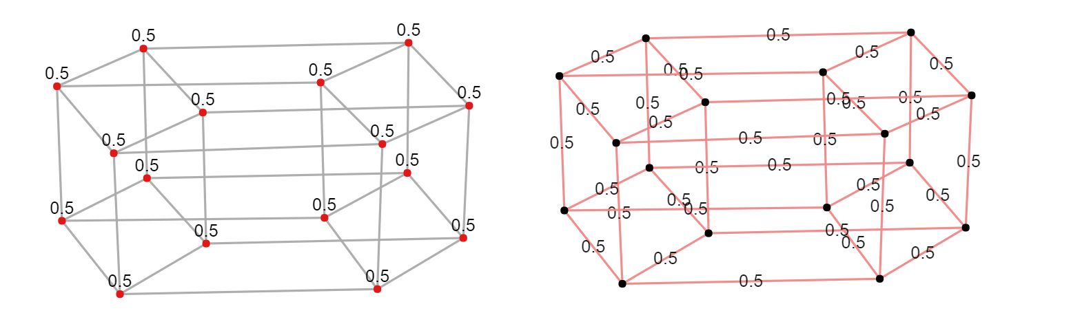
Refer to caption
Figure 1.2: Bakry-Émery and Ollivier’s Ricci curvature of the hypercube graph Q4Q^{4}
Example 1.20.

The antitree graph is the infinite graph constructed by placing complete graphs KnK_{n}, n=1,2,3,…n=1,2,3,... (in an increasing order of nn) and connecting every vertex of KiK_{i} to every vertex of Ki+1K_{i+1} for all i∈ℕi\in\mathbb{N}. The antitree graph represents a (elliptic) paraboloid. A paraboloid is a manifold with positive curvature everywhere, but its curvature is reaching zero at a point further away from the paraboloid’s vertex. It is good to note that Bonnet-Myers theorem does not apply, and a paraboloid is indeed non-compact. As shown in Figure 1.3, the curvature of the antitree is calculated to be {0.5, 0.212, 0.092, 0.049, …} in Bakry-Émery curvature and {0.6, 0.15, 0.068, 0.039, …} in Ollivier’s Ricci curvature. This calculation suggests evidentially that the antitree is an infinite graph whose curvature is also reaching zero. A precise formula to calculate curvature of a generalized family of antitrees can be found in [11].

Refer to caption
Figure 1.3: Bakry-Émery and Ollivier’s Ricci curvature of the antitree graph
Example 1.21.

A dumbbell graph is a graph obtained by connecting two complete graphs KnK_{n} and KmK_{m} with a single edge. Such edge represents a “bottleneck” of a manifold. In general, a bottleneck of a manifold is negatively curved (i.e. in a saddle shape), and as expected, a dumbbell graph also has negative curvature around its bottleneck, as shown in Figure 1.4.

Refer to caption
Figure 1.4: Bakry-Émery and Ollivier’s Ricci curvature of a dumbbell graph

Chapter 2 Combinatorial Curvature

The idea behind Gauss-Bonnet Theorem comes from a relation between the sum of interior angles of a triangle (formed by three geodesics) on a surface and the total curvature inside that triangle (see [14]). When a surface is triangulated (i.e. partitioned into small triangles, or polygons), it resembles planar graphs. Gaussian curvature, which explains angles on surfaces, is translated into combinatorial curvature, which explains “angles” in planar graphs. Hence these two curvature notions describe the geometry of surfaces very similarly.

2.1 Planar tessellations

We shall start with the definition of graphs. A graph GG, written as G=(V,E)G=(V,E) consists of a set VV of elements called vertices (singular: vertex), and a set EE whose elements are edge, each of which connects a pair of vertices (called endpoints of an edge). Throughout this paper, we assume graphs to be undirected, which means edges have no direction, and to be simple, which means they contain no loop (i.e. an edge whose endpoints are the same vertex) and no multiple edges (i.e. more than one edges sharing the same pair of endpoints). When vertices uu and vv are connected by one (and only) edge ee in EE, we may say that uu is adjacent to vv (written as u∼vu\sim v or u∼evu\stackrel{{\scriptstyle e}}{{\sim}}v). For a vertex v∈Vv\in V, the degree of vv, denoted by dvd_{v}, is the number of vertices that are adjacent to vv. A (finite) path is a sequence of (finite) edges which connect a sequence of all distinct vertices (except possibly the first and the last):

v1∼e1v2∼e2v3∼e3…∼en−1vn.v_{1}\stackrel{{\scriptstyle e_{1}}}{{\sim}}v_{2}\stackrel{{\scriptstyle e_{2}}}{{\sim}}v_{3}\stackrel{{\scriptstyle e_{3}}}{{\sim}}...\stackrel{{\scriptstyle e_{n-1}}}{{\sim}}v_{n}.

The length of a path is the number of edges in its sequence. For two vertices uu and vv, the combinatorial distance function d⁡(u,v)d(u,v) is defined to be the length of shortest path connecting uu and vv. By convention, set d⁡(u,u)=0d(u,u)=0 for all vertices uu, and set d⁡(u,v)=∞d(u,v)=\infty if there is no path connecting uu and vv. Moreover, a graph is said to be connected if, for every pair of vertices uu and vv, there exists a path connecting uu and vv.

In the setup of combinatorial curvature, graphs are required to be 𝑝𝑙𝑎𝑛𝑎𝑟\it{planar}, so that the notion of faces can be introduced. A planar graph is a graph G=(V,E)G=(V,E) that can be embedded in ℝ2\mathbb{R}^{2} without self intersecting edges. The union of edges ⋃e∈Ee\bigcup_{e\in E}e, when realized in ℝ2\mathbb{R}^{2}, divides the entire space ℝ2\mathbb{R}^{2} into connected components. The closure of each component in ℝ2\⋃e∈Ee\mathbb{R}^{2}\backslash\bigcup_{e\in E}e is called a 𝑓𝑎𝑐𝑒\it face. Let FF be the set of all faces, so we may consider it as an additional structure of a planar graph GG: G=(V,E,F)G=(V,E,F). We further assume graphs to be locally finite. A planar graph GG is locally finite if every point of ℝ2\mathbb{R}^{2} has an open neighborhood intersecting only finitely many faces of GG. Local finiteness prevents graphs from clustering in arbitrarily small area.

In [2], O. Baues and N. Peyerimhoff define conditions for locally finite planar graphs to be tessellations as follows.

Definition 2.1 (Tessellation).

A connected and locally finite planar graph GG is a planar tessellation, or just tessellation, if it satisfies the following conditions.

  • (i)

    Every edge is contained in exactly two different faces.

  • (ii)

    Every bounded face is a polygon: it is homeomorphic to the closed disk 𝔻¯\overline{\mathbb{D}}, and its boundary is a simple cycle (i.e. a finite path in which the first and the last vertices coincide). The edges of the cycle are called sides of the polygon.

  • (iii)

    The intersection of any two distinct faces are either an empty set, or a vertex, or an edge.

Condition (iii) suggests the convexity property for polygons. Figure 2.1 shows two examples where the condition (iii) breaks.

Refer to caption
Figure 2.1: Polygonal faces violating tessellation rule
Remark 2.2.

There are two cases of planar tessellations that we are interested in. First is an infinite tessellation: it contains infinitely many faces, and every face is bounded. Second is a finite tessellation: it contains exactly one unbounded face, which is homeomorphic to ℝ2\𝔻\mathbb{R}^{2}\backslash\mathbb{D} and its boundary is a simple cycle. In case of a finite tessellation, by realizing ℝ2∪{∞}\mathbb{R}^{2}\cup\{\infty\} as a 2-dimensional sphere S2S^{2}, the unbounded face can be viewed as a bounded polygon (containing the point at infinity). Thus, in fact, a finite planar can be realized as a finite tessellation of S2S^{2}.

For a face f∈Ff\in F of a tessellation, let dfd_{f} denote its degree: the number of vertices (or equivalently, the number of sides) of the boundary of polygon ff. The conditions on tessellations imply that 3≤dv<∞3\leq d_{v}<\infty, and 3≤df<∞3\leq d_{f}<\infty for all v∈Vv\in V, f∈Ff\in F.

Two combinatorial curvature notations are defined as follows.

Definition 2.3 (Combinatorial curvature).

For each vertex vv and a face ff having vv as its vertex (written as f∼vf\sim v), the corner curvature is defined as

κ⁡(v,f)=1dv+1df−12.\kappa(v,f)=\frac{1}{d_{v}}+\frac{1}{d_{f}}-\frac{1}{2}.

For a vertex vv, the (vertex) curvature is

κ(v)=∑f:f∼vκ(v,f).\kappa(v)=\sum\limits_{f:f\sim v}\kappa(v,f).

summed over all faces ff having vv as their vertex.

In fact, for a fixed vertex vv, the number of faces ff incident to vv is equal to its degree |v||v|. Hence, the (vertex) curvature can be defined in another way as

κ(v)=∑f:f∼v(1dv+1df−12)=1−dv2+∑f:f∼v1df\kappa(v)=\sum\limits_{f:f\sim v}\left(\frac{1}{d_{v}}+\frac{1}{d_{f}}-\frac{1}{2}\right)=1-\frac{d_{v}}{2}+\sum\limits_{f:f\sim v}\frac{1}{d_{f}}

The motivation behind this definition of curvature is “angular defect”, which can be explained as follows. If each face ff were to be realized as a regular polygon of equal side length, the inner angle of polygon ff would be (1−2df)​π(1-\frac{2}{d_{f}})\pi and the sum of angles of all faces ff’s at the vertex vv would then be

∑f:f∼v(1−2df)π=2π(dv2−∑f:f∼v1df)=2π(1−κ(v)).\sum\limits_{f:f\sim v}\bigg(1-\frac{2}{d_{f}}\bigg)\pi=2\pi\bigg(\frac{d_{v}}{2}-\sum\limits_{f:f\sim v}\frac{1}{d_{f}}\bigg)=2\pi(1-\kappa(v)).

If κ⁡(v)<0\kappa(v)<0, then the sum of angles at vv is more than 2​π2\pi, which means that these polygonal faces around vv form a saddle-shape surface around vv. On the other hand, when κ⁡(v)>0\kappa(v)>0, the sum of angles at vv is less than 2​π2\pi, and therefore the point vv behaves like an elliptical point. In other words, the sign of κ⁡(v)\kappa(v) (negative/zero/positive) corresponds to the geometry of the surface at point vv (hyperbolic/euclidean/spherical).

2.2 Combinatorial Gauss-Bonnet and Cartan-Hadamard

In Riemannian geometry, Gauss-Bonnet theorem states that for a closed surface MM, the total curvature of SS can be related to its Euler’s characteristic by the formula (see Section 1.1):

∫MK​d​A=2​π​χ​(M).\int_{M}K\ \textup{d}A=2\pi\chi(M).

In a case when GG is a finite planar tessellation, or equivalently a finite tessellation of S2S^{2} (see Remark 2.2), the Euler’s characteristic of GG is given by χ⁡(G)=χ⁡(S2)=2\chi(G)=\chi(S^{2})=2. Gauss-Bonnet theorem has the following discrete analogue for a finite planar tessellation.

Theorem 2.4 (Combinatorial Gauss-Bonnet).

Let G=(V,E,F)G=(V,E,F) be a finite planar tessellation. Then ∑v∈Vκ⁡(v)=2\sum\limits_{v\in V}\kappa(v)=2.

Proof.
∑v∈Vκ⁡(v)\displaystyle\sum\limits_{v\in V}\kappa(v) =∑v∈V(1−dv2+∑f:f∼v1df)\displaystyle=\sum\limits_{v\in V}\bigg(1-\frac{d_{v}}{2}+\sum\limits_{f:f\sim v}\frac{1}{d_{f}}\bigg)
=|V|−12∑v∈Vdv+∑v∈V∑f:f∼v1df\displaystyle=|V|-\frac{1}{2}\sum\limits_{v\in V}d_{v}+\sum\limits_{v\in V}\sum\limits_{f:f\sim v}\frac{1}{d_{f}}
=|V|−|E|+∑f∈F∑v:f∼v1df\displaystyle=|V|-|E|+\sum\limits_{f\in F}\sum\limits_{v:f\sim v}\frac{1}{d_{f}}
=|V|−|E|+∑f∈F1\displaystyle=|V|-|E|+\sum\limits_{f\in F}1
=|V|−|E|+|F|\displaystyle=|V|-|E|+|F|
=2\displaystyle=2

We use the fact that ∑v∈Vdv=2​|E|\sum_{v\in V}d_{v}=2|E|, since each edge is counted twice in the sum. Moreover, the order of double summations is interchangeable since the sets VV and FF are finite. Lastly, |V|−|E|+|F|=2|V|-|E|+|F|=2 is the Euler’s characteristic formula applied for a finite connected planar graph. ∎

Next, we investigate graphs that have the same sign of curvatures everywhere. Let us start with non-positively curved graphs.

Corollary 2.5.

A tessellation that has non-positive curvature at every vertex must be infinite.

Proof.

Follows immediately from Gauss-Bonnet formula. ∎

Next theorem is a main result from Baues and Peyerimhoff’s paper [2, Theorem 1], which is considered as a discrete analogue of Cartan-Hadamard theorem in Riemannian geometry. We omit the proof of this theorem.

Theorem 2.6 (Combinatorial Cartan-Hadamard).

Let G=(V,E,F)G=(V,E,F) be a tessellation. For a fixed vertex v0∈Vv_{0}\in V, define the cut locus of f0f_{0} to be

C⁡(v0):={v′∈F:d⁡(v0,v′)≤d⁡(v0,v)​ for all neighbors ​v​ of ​v′}C(v_{0}):=\Big\{v^{\prime}\in F:d(v_{0},v^{\prime})\leq d(v_{0},v)\textup{ for all neighbors }v\textup{ of }v^{\prime}\Big\}

If κ⁡(v,f)≤0\kappa(v,f)\leq 0 for every corner (v,f)(v,f), then GG has no cut locus, i.e. C⁡(v0)=∅C(v_{0})=\emptyset for all v0∈Vv_{0}\in V.

In words, the theorem asserts that, when using any vertex v0v_{0} as a base point, there exists no vertex xx where the distance function dv0​(x):=d⁡(v0,x)d_{v_{0}}(x):=d(v_{0},x) attains the local maxima. Equivalently, it means that every geodesic (starting at any v0v_{0}) can be extended infinitely, as similarly stated in the theorem of Cartan-Hadamard (see Theorem 1.2).

2.3 Cheeger constant and isoperimetric inequality on graphs

In Section 1.1, we learn that a simply connected and complete surface MM with negative (sectional) curvatures uniformly bounded above by −K0<0-K_{0}<0 (hence MM is non-compact by Cartan-Hadarmard theorem) satisfies the isoperimetric inequality:

area​(H)≤1K0⋅length​(∂H).\textup{area}(H)\leq\frac{1}{\sqrt{K_{0}}}\cdot\textup{length}(\partial H).

for all compact surfaces H⊂MH\subset M with boundary ∂H\partial H (see Theorem 1.5).

In graphs, Cheeger constant can be defined and the isoperimetric inequality can be read analogously as in the following definition and theorem.

Definition 2.7 (Combinatorial Cheeger constant).

Let G=(V,E)G=(V,E) be a graph. For a finite subset W⊂VW\subset V, let ∂EW\partial_{E}W be the set containing all edges which connect a vertex in WW to a vertex in V\WV\backslash W, and define the volume of WW as vol​(W):=∑v∈Wdv\mbox{vol}(W):=\sum\limits_{v\in W}d_{v}.
The Cheeger constant is then defined to be

α⁡(G):=infW|∂EW|vol​(W)\alpha(G):=\inf_{W}\frac{|\partial_{E}W|}{\textup{vol}(W)}

where the infimum is taken over all finite subset W⊂VW\subset V such that |W|≤12​|V||W|\leq\frac{1}{2}|V|. Moreover, if GG is infinite (|V|=∞|V|=\infty), then the constraint |W|<12​|V||W|<\frac{1}{2}|V| may be removed.

Theorem 2.8.

Let G=(V,E,F)G=(V,E,F) be a planar tessellation. Suppose there exists a constant K0>0K_{0}>0 such that the corner curvature κ⁡(v,f)≤−K0<0\kappa(v,f)\leq-K_{0}<0 holds for every corner (v,f)(v,f). Then α⁡(G)≥2​K0\alpha(G)\geq 2K_{0}.

A proof of this theorem with a more precise bound on α⁡(G)\alpha(G) can be found in Keller and Peyerimhoff’s paper [20, Theorem 1].

Proof.

First of all, GG is infinite, by Corollary 2.5. For any finite subset W⊆VW\subseteq V, let GW=(W,EW)G_{W}=(W,E_{W}) denote the finite subgraph of GG induced by WW, such that EW⊆EE_{W}\subseteq E is the set of all edges with both endpoints in WW. As a subgraph of a planar graph, GWG_{W} is also planar, and hence inducing the set of faces, namely FWF_{W}. It is not always true that FW⊆FF_{W}\subseteq F, in particular, if the tessellation is infinite.

This proof involves two steps. Firstly, for given any finite W⊆VW\subseteq V, we choose a particular W′⊆VW^{\prime}\subseteq V with |∂EW′|vol​(W′)≤|∂EW|vol​(W)\frac{|\partial_{E}W^{\prime}|}{\mbox{vol}(W^{\prime})}\leq\frac{|\partial_{E}W|}{\mbox{vol}(W)}. The second step is to show that our choice of W′W^{\prime} satisfies |∂EW′|vol​(W′)≥2​K0\frac{|\partial_{E}W^{\prime}|}{\mbox{vol}(W^{\prime})}\geq 2K_{0}.

Part 1 Suppose GWG_{W} has nn connected components, namely GWi=(Wi,EWi)G_{W_{i}}=(W_{i},E_{W_{i}}) for i=1,⋯,ni=1,\cdots,n. Observe that

|∂EW|=∑i=1n|∂EWi|​ and vol​(W)=∑i=1nvol​(Wi).|\partial_{E}W|=\sum\limits_{i=1}^{n}|\partial_{E}W_{i}|\mbox{\ \ \ \ \ \ \ and\ \ \ \ \ \ \ }\mbox{vol}(W)=\sum\limits_{i=1}^{n}\mbox{vol}(W_{i}).

Without loss of generality, assume that W1W_{1} has the minimum isoperimetric ratio:

c1:=|∂EW1|vol​(W1)=min1≤i≤n⁡|∂EWi|vol​(Wi).c_{1}:=\frac{|\partial_{E}W_{1}|}{\mbox{vol}(W_{1})}=\min\limits_{1\leq i\leq n}\frac{|\partial_{E}W_{i}|}{\mbox{vol}(W_{i})}.

It follows that

|∂EW|vol​(W)=∑i=1n|∂EWi|∑i=1nvol​(Wi)≥c1=|∂EW1|vol​(W1).\frac{|\partial_{E}W|}{\mbox{vol}(W)}=\dfrac{\sum\limits_{i=1}^{n}|\partial_{E}W_{i}|}{\sum\limits_{i=1}^{n}\mbox{vol}(W_{i})}\geq c_{1}=\frac{|\partial_{E}W_{1}|}{\mbox{vol}(W_{1})}.

Next, construct a set W′⊆VW^{\prime}\subseteq V by adding into the set W1W_{1} all vertices v∈Vv\in V (if they exist) such that vv lies in UU, the union of all bounded faces of GW1G_{W_{1}}. Now consider the induced subgraph GW′=(W′,EW′)G_{W^{\prime}}=(W^{\prime},E_{W^{\prime}}) with the set of faces FW′F_{W^{\prime}}. Geometrically, the difference between the graph GW1G_{W_{1}} and GW′G_{W^{\prime}} is that GW1G_{W_{1}} was connected but may not have been a tessellation, whereas GW′G_{W^{\prime}} is "simply connected" and it is a tessellation. Figure 2.2 shows an example when GW1G_{W_{1}} has a non-polygonal face, but GW′G_{W^{\prime}} has nicely tessellating faces. Note that ∂EW′⊆∂EW1\partial_{E}{W^{\prime}}\subseteq\partial_{E}W_{1}. Hence,

|∂EW1|vol​(W1)≥|∂EW′|vol​(W′).\frac{|\partial_{E}W_{1}|}{\mbox{vol}(W_{1})}\geq\frac{|\partial_{E}W^{\prime}|}{\mbox{vol}(W^{\prime})}.
Refer to caption
Figure 2.2: A non-polygonal face in GW1G_{W_{1}} and 12 faces in GW′G_{W^{\prime}}

Each bounded face of GW′G_{W^{\prime}} has no vertex v∈Vv\in V in its interior, because otherwise vv would be included in W′W^{\prime} in the construction step. In other words, each bounded face of GW′G_{W^{\prime}} also belongs to GG. Moreover, GW′G_{W^{\prime}} has only one unbounded face. This unbounded face must not be a face of GG; otherwise, all faces of GW′G_{W^{\prime}} and all faces of GG coincide, which then implies that GW′=GG_{W^{\prime}}=G. This is impossible, since GW′G_{W^{\prime}} is finite but GG is infinite. Therefore,

|FW′|−|FW′∩F|=1.|F_{W^{\prime}}|-|F_{W^{\prime}}\cap F|=1.

Part 2 The assumption on κ⁡(v,f)\kappa(v,f) implies that for any finite W⊆VW\subseteq V,

∑v∈Wκ⁡(v)≤−K0​vol​(W)\displaystyle\sum\limits_{v\in W}\kappa(v)\leq-K_{0}\mbox{vol}(W) (2.1)

By definition of curvature,

∑v∈Wκ⁡(v)\displaystyle\sum\limits_{v\in W}\kappa(v) =∑v∈W(1−dv2+∑f∈Ff∼v1df)\displaystyle=\sum\limits_{v\in W}\bigg(1-\frac{d_{v}}{2}+\sum\limits_{\begin{subarray}{c}f\in F\\ f\sim v\end{subarray}}\frac{1}{d_{f}}\bigg)
=|W|−12​∑v∈Wdv+∑v∈W∑f∈Ff∼v1df\displaystyle=|W|-\frac{1}{2}\sum\limits_{v\in W}d_{v}+\sum\limits_{v\in W}\sum\limits_{\begin{subarray}{c}f\in F\\ f\sim v\end{subarray}}\frac{1}{d_{f}} (2.2)

whereas

∑v∈Wdv=2​|EW|+|∂EW|\sum\limits_{v\in W}d_{v}=2|E_{W}|+|\partial_{E}W| (2.3)

because each edge in EWE_{W} has both endpoints in WW and each edge in ∂EW\partial_{E}W has exactly one endpoint in WW. Moreover,

∑v∈W∑f∈Ff∼v1df≥∑f∈FW∩F∑v∈Wf∼v1df=∑f∈FW∩F1=|FW∩F|\sum\limits_{v\in W}\sum\limits_{\begin{subarray}{c}f\in F\\ f\sim v\end{subarray}}\frac{1}{d_{f}}\geq\sum\limits_{\begin{subarray}{c}f\in F_{W}\cap F\end{subarray}}\sum\limits_{\begin{subarray}{c}v\in W\\ f\sim v\end{subarray}}\frac{1}{d_{f}}=\sum\limits_{\begin{subarray}{c}f\in F_{W}\cap F\end{subarray}}1=|F_{W}\cap F| (2.4)

since we restrict the sum to be summed only over the faces f∈FW∩Ff\in F_{W}\cap F, each of which is a polygon whose vertices are in WW.

Combining (2.2), (2.3), and (2.4), we obtain

∑v∈Wκ⁡(v)≥|W|−|EW|−|∂EW|2+|FW∪F|.\displaystyle\sum\limits_{v\in W}\kappa(v)\geq|W|-|E_{W}|-\frac{|\partial_{E}W|}{2}+|F_{W}\cup F|.

In particular, for our choice of W′⊂VW^{\prime}\subset V from Part 1 we have

−K0​vol​(W′)\displaystyle-K_{0}\mbox{vol}(W^{\prime}) ≥|W′|−|EW′|−|∂EW′|2+|FW′|−1\displaystyle\geq|W^{\prime}|-|E_{W^{\prime}}|-\frac{|\partial_{E}W^{\prime}|}{2}+|F_{W^{\prime}}|-1
=1−|∂EW′|2\displaystyle=1-\frac{|\partial_{E}W^{\prime}|}{2}

where the last equality applies Euler’s formula |W′|−|EW′|+|FW′|=2|W^{\prime}|-|E_{W^{\prime}}|+|F_{W^{\prime}}|=2 for a finite connected planar graph W′W^{\prime}.

We can now conclude |∂EW′|vol​(W′)≥2​K0\frac{|\partial_{E}W^{\prime}|}{\mbox{vol}(W^{\prime})}\geq 2K_{0} as desired. ∎

2.4 Combinatorial Bonnet-Myers

At the end of [17], Higuchi conjectures that everywhere positive combinatorial curvature implies the finiteness of graphs. This conjecture can be regarded as a discrete analogue to a weak version of the Bonnet-Myers theorem.

Conjecture 2.9 (Higuchi).

A tessellation that has positive curvature at every vertex must be a finite graph.

Let us investigate two examples of tessellations, namely 𝑝𝑟𝑖𝑠𝑚\it prism and 𝑎𝑛𝑡𝑖𝑝𝑟𝑖𝑠𝑚\it antiprism.
A prism is a graph with 2​n2n vertices u1,v1,u2,v2,…,un,vnu_{1},v_{1},u_{2},v_{2},...,u_{n},v_{n} with edges joining

u1∼u2∼…∼un∼u1​ and ​v1∼v2∼…∼vn∼v1​ and ​ui∼viu_{1}\sim u_{2}\sim...\sim u_{n}\sim u_{1}\mbox{ and }v_{1}\sim v_{2}\sim...\sim v_{n}\sim v_{1}\mbox{ and }u_{i}\sim v_{i}

for all 1≤i≤n1\leq i\leq n. Its faces consist of two nn-gons, and nn quadrilaterals. See Figure 2.3.

Refer to caption
Figure 2.3: Prism and its embedding in ℝ2\mathbb{R}^{2}

In its embedding in ℝ2\mathbb{R}^{2}, the unbounded component represents one of the two nn-gonal faces. For every vertex vv of the prism, there are one nn-gon and two quadrilaterals incident to it. Hence the combinatorial curvature can be calculated by

κ⁡(v)=1−32+(14+14+1n)=1n>0.\kappa(v)=1-\frac{3}{2}+\bigg(\frac{1}{4}+\frac{1}{4}+\frac{1}{n}\bigg)=\frac{1}{n}>0.

An antiprism can be constructed from a prism with additional edges ui∼vi+1u_{i}\sim v_{i+1} for 1≤i≤n−11\leq i\leq n-1 and un∼v1u_{n}\sim v_{1}. It has two nn-gonal faces, and 2​n2n triangular faces. See Figure 2.4.

Refer to caption
Figure 2.4: Antiprism and its embedding in ℝ2\mathbb{R}^{2}

Each vertex vv of an antiprism has one nn-gon and three quadrilaterals incident to it, so the curvature is

κ⁡(v)=1−42+(13+13+13+1n)=1n>0.\kappa(v)=1-\frac{4}{2}+\bigg(\frac{1}{3}+\frac{1}{3}+\frac{1}{3}+\frac{1}{n}\bigg)=\frac{1}{n}>0.

As shown above, prism and antiprism demonstrate two classes of tessellations that have positive curvature everywhere. Although both prism and antiprism are finite graphs, their numbers of vertices can be arbitrary large. In [12], DeVos and Mohar proved Higuchi’s conjecture and provided a further insight about the finiteness that: all everywhere-positively-curved tessellation (except prisms and antiprisms) have a uniform upper bound on the number of their vertices, and they asked for a sharp bound. In [24], the authors gives an example of one such graph with 208208 vertices. On the other hand, it was recently proved in [15] that all such graphs have at most 208 vertices, hence 208 is the optimal number.

Theorem 2.10 (Combinatorial Bonnet-Myers).

If κ⁡(v)>0\kappa(v)>0 for every vertex vv in a planar graph G=(V,E)G=(V,E), then GG is finite. Moreover, GG is either a prism, antiprism, or |V|≤208|V|\leq 208.

Chapter 3 Bakry-Émery Curvature

While the previous curvature notion was based on a discrete version of the Gauss-Bonnet Theorem in two-dimension, the curvature notion in this chapter, introduced by D. Bakry and M. Émery [1], is based on Bochner’s formula from Riemannian geometry. Graphs are no longer assumed to be planar, and their dimensions are not restricted to two. Instead, the dimension can be chosen to be an arbitrary positive real number, including ∞\infty.

3.1 CD inequality and Γ\Gamma-calculus

Bochner’s formula states that for every smooth real function f∈C∞​(M)f\in C^{\infty}(M) and at every point x∈Mx\in M,

12​Δ​|grad ​f|2​(x)=‖Hess ​f‖2​(x)+⟨grad ​Δ​f​(x),grad ​f​(x)⟩+Ric​(grad ​f​(x)),\frac{1}{2}\Delta|\textup{grad }f|^{2}(x)=\|\textup{Hess }f\|^{2}(x)+\langle\textup{grad }\Delta f(x),\textup{grad }f(x)\rangle+\mbox{Ric}(\textup{grad }f(x)), (3.1)

Further, defined at each point xx the curvature term Kx:=infv∈Tx​MRic​(v)|v|2K_{x}:=\inf\limits_{v\in T_{x}M}\frac{\textup{Ric}(v)}{|v|^{2}} which gives a lower bound for Ricci curvature term:

Ric​(grad ​f​(x))≥Kx​|grad ​f​(x)|2.\textup{Ric}(\textup{grad }f(x))\geq K_{x}|\textup{grad }f(x)|^{2}.

Recall also Proposition 1.13: ‖Hess ​f‖2​(x)≥1n​(Δ​f​(x))2\displaystyle\|\textup{Hess }f\|^{2}(x)\geq\frac{1}{n}(\Delta f(x))^{2}. Combining these two inequalities into the equation (3.1), we have the so called "curvature-dimension" inequality,

12​Δ​|grad ​f|2​(x)−⟨grad ​Δ​f​(x),grad ​f​(x)⟩≥1n​(Δ​f​(x))2+Kx​|grad ​f​(x)|2\frac{1}{2}\Delta|\textup{grad }f|^{2}(x)-\langle\textup{grad }\Delta f(x),\textup{grad }f(x)\rangle\geq\frac{1}{n}(\Delta f(x))^{2}+K_{x}|\textup{grad }f(x)|^{2} (3.2)

According to [1], define bilinear operators Γ\Gamma and Γ2\Gamma_{2} as follows.

Definition 3.1 (Γ\Gamma and Γ2\Gamma_{2} notions).

For f,g∈C∞​(M)f,g\in C^{\infty}(M), define

2​Γ​(f,g)​(x):=Δ⁡(f​g)​(x)−f⁡(x)⋅Δ​g​(x)−Δ​f​(x)⋅g⁡(x)2\Gamma(f,g)(x):=\Delta(fg)(x)-f(x)\cdot\Delta g(x)-\Delta f(x)\cdot g(x) (3.3)
2​Γ2​(f,g)​(x):=Δ​Γ​(f,g)​(x)−Γ⁡(f,Δ​g)​(x)−Γ⁡(Δ​f,g)​(x)2\Gamma_{2}(f,g)(x):=\Delta\Gamma(f,g)(x)-\Gamma(f,\Delta g)(x)-\Gamma(\Delta f,g)(x) (3.4)

In fact, Γ⁡(f,g)​(x)=2​⟨grad ​f​(x),grad ​g​(x)⟩\Gamma(f,g)(x)=2\langle\textup{grad }f(x),\textup{grad }g(x)\rangle by the product rule (see Proposition 1.10). We further denote Γ⁡(f):=Γ⁡(f,f)\Gamma(f):=\Gamma(f,f), and Γ2​(f):=Γ2​(f,f)\Gamma_{2}(f):=\Gamma_{2}(f,f). The curvature-dimension inequality (3.2) can then be rewritten as

Γ2​(f)​(x)≥1n​(Δ​f​(x))2+Kx​Γ​(f)​(x)\Gamma_{2}(f)(x)\geq\frac{1}{n}(\Delta f(x))^{2}+K_{x}\Gamma(f)(x) (3.5)

which holds for all f∈C∞​(M)f\in C^{\infty}(M) and x∈Mx\in M.

Observe that the above curvature-dimension inequality involves the Γ\Gamma and Γ2\Gamma_{2} terms, which were defined merely via the Laplacian. This allows us to consider curvature-dimension property on any space, once the Laplacian is specified on such space.

Definition 3.2.

Let XX be a space and C⁡(X)C(X) be the function space of XX, that is the set of all functions f:X→ℝf:X\rightarrow\mathbb{R}, equipped with the addition and scalar multiplication rules: (f+f′)​(x)=f⁡(x)+f′​(x)(f+f^{\prime})(x)=f(x)+f^{\prime}(x) and (c​f)​(x)=c⋅f​(x)(cf)(x)=c\cdot f(x). Assume that the XX has Laplacian operator Δ\Delta defined on it. Fix a number n∈ℝ+∪{∞}n\in\mathbb{R}^{+}\cup\{\infty\} to be the dimension of XX. The curvature at each point x∈Xx\in X is defined to be the maximal number KxK_{x} such that the inequality

Γ2​(f)​(x)≥1n​(Δ​f​(x))2+Kx​Γ​(f)​(x)\Gamma_{2}(f)(x)\geq\frac{1}{n}(\Delta f(x))^{2}+K_{x}\Gamma(f)(x) (3.6)

holds true for all functions f∈C⁡(X)f\in C(X)

Moreover, for a fixed real number KK, we say that XX satisfies C​D​(K,n)CD(K,n) if Kx≥KK_{x}\geq K for all x∈Xx\in X; in other words,

Γ2​(f)​(x)≥1n​(Δ​f​(x))2+K​Γ​(f)​(x)\Gamma_{2}(f)(x)\geq\frac{1}{n}(\Delta f(x))^{2}+K\Gamma(f)(x) (3.7)

holds for all x∈Xx\in X and for all f∈C⁡(X)f\in C(X).
Here the operators Γ\Gamma and Γ2\Gamma_{2} on XX are also defined as in the equation (3.3) and (3.4).

In particular, Laplacian on graphs can be specified as follows.

Definition 3.3 (Discrete Laplacian).

Let G=(V,E)G=(V,E) be a graph with finite degree on each vertex. Laplacian Δ:C⁡(V)→C⁡(V)\Delta:C(V)\rightarrow C(V) is a linear operator, defined on any function f:V→ℝf:V\rightarrow\mathbb{R} as

Δ​f​(x):=1dx​∑z∼x(f⁡(z)−f⁡(x))\Delta f(x):=\frac{1}{d_{x}}\sum\limits_{z\sim x}\bigg(f(z)-f(x)\bigg)

for all vertices x∈Vx\in V. In terms of matrix representation, we can write Laplacian as

Δ=D−1​(A−Id)\Delta=D^{-1}(A-\textup{Id})

where DD is the diagonal matrix whose entries are the vertex degrees: Dx​x=dxD_{xx}=d_{x}, and AA is the agjacency matrix: Ax​y=1A_{xy}=1 if x∼yx\sim y and 0 otherwise.

This notion is sometimes called the normalized Laplacian (in contrast to the non-normalized one, where the factor 1dx\frac{1}{d_{x}} is dropped). Here are some properties of operators Δ\Delta and Γ\Gamma defined on graphs.

Proposition 3.4.

Let G=(V,E)G=(V,E) be a graph. For f,g∈C⁡(V)f,g\in C(V), we have

  • (a)
    2​Γ​(f,g)​(x)=1dx​∑z∼x(f⁡(z)−f⁡(x))​(g⁡(z)−g⁡(x)).2\Gamma(f,g)(x)=\frac{1}{d_{x}}\sum\limits_{z\sim x}\bigg(f(z)-f(x)\bigg)\bigg(g(z)-g(x)\bigg).

    In particular,

    2​Γ​(f)​(x)=1dx​∑z∼x(f⁡(z)−f⁡(x))2.2\Gamma(f)(x)=\frac{1}{d_{x}}\sum\limits_{z\sim x}\bigg(f(z)-f(x)\bigg)^{2}.
  • (b)

    (Δ​f​(x))2≤2​Γ​f​(x)(\Delta f(x))^{2}\leq 2\Gamma f(x) for all f∈C⁡(V)f\in C(V) and x∈Vx\in V.

  • (c)

    If GG is finite, then

    ∑x∈Vdx​Δ​f​(x)=0\sum\limits_{x\in V}d_{x}\Delta f(x)=0

    for all f∈C⁡(V)f\in C(V).

Proof.

  • (a)

    Straightforward calculation from the definition gives

    2​Γ​(f,g)​(x)\displaystyle 2\Gamma(f,g)(x) =Δ⁡(f​g)​(x)−f⁡(x)⋅Δ​g​(x)−Δ​f​(x)⋅g⁡(x)\displaystyle=\Delta(fg)(x)-f(x)\cdot\Delta g(x)-\Delta f(x)\cdot g(x)
    =1dx∑z∼x[(f(z)g(z)−f(x)g(x))\displaystyle=\frac{1}{d_{x}}\sum\limits_{z\sim x}\bigg[\bigg(f(z)g(z)-f(x)g(x)\bigg)
    −f(x)(g(z)−g(x))−g(x)(f(z)−f(x))]\displaystyle\ \ \ \ \ \ \ \ \ \ \ \ \ \ \ -f(x)\bigg(g(z)-g(x)\bigg)-g(x)\bigg(f(z)-f(x)\bigg)\bigg]
    =1dx​∑z∼x(f⁡(z)−f⁡(x))​(g⁡(z)−g⁡(x)).\displaystyle=\frac{1}{d_{x}}\sum\limits_{z\sim x}\bigg(f(z)-f(x)\bigg)\bigg(g(z)-g(x)\bigg).

    The second identity in part (a) follows immediately.

  • (b)

    From Arithmetic-Quadratic mean (AM-QM) inequality,

    |Δ​f​(x)|≤1dx​∑z∼x|f⁡(z)−f⁡(x)|≤1dx​∑z∼x(f⁡(z)−f⁡(x))2=(a)2​Γ​f​(x).|\Delta f(x)|\leq\frac{1}{d_{x}}\sum\limits_{z\sim x}\bigg|f(z)-f(x)\bigg|\leq\sqrt{\frac{1}{d_{x}}\sum\limits_{z\sim x}\bigg(f(z)-f(x)\bigg)^{2}}\stackrel{{\scriptstyle(a)}}{{=}}\sqrt{2\Gamma f(x)}.
  • (c)

    Suppose GG is finite.

    ∑x∈Vdx​Δ​f​(x)\displaystyle\sum\limits_{x\in V}d_{x}\Delta f(x) =∑x∈V∑z:z∼x(f(z)−f(x))\displaystyle=\sum\limits_{x\in V}\sum\limits_{z:z\sim x}\bigg(f(z)-f(x)\bigg)
    =∑x∈V∑z:z∼xf(z)−∑x∈Vdxf(x)\displaystyle=\sum\limits_{x\in V}\sum\limits_{z:z\sim x}f(z)-\sum\limits_{x\in V}d_{x}f(x)
    =∑z∈V∑x:z∼xf(z)−∑x∈Vdxf(x)\displaystyle=\sum\limits_{z\in V}\sum\limits_{x:z\sim x}f(z)-\sum\limits_{x\in V}d_{x}f(x)
    =∑z∈Vdz​f​(z)−∑x∈Vdx​f​(x)=0\displaystyle=\sum\limits_{z\in V}d_{z}f(z)-\sum\limits_{x\in V}d_{x}f(x)=0

∎

In Section 1.3, we obtain Lichnerowicz’s bound on first nonzero eigenvalue by taking integral on the Bochner’s formula and applying the Divergence theorem. Here, we imitate a similar result in a discrete analogue.

Theorem 3.5 (B-E Lichnerowicz).

Let G=(V,E)G=(V,E) be a finite connected graph satisfying C​D​(K,n)CD(K,n) condition for some K>0K>0. Then the first nonzero eigenvalue with respect to the Laplacian operator Δ\Delta satisfies λ1≥nn−1​K\lambda_{1}\geq\frac{n}{n-1}K.

In fact, the condition that GG is finite can be removed, since the condition C​D​(K,n)CD(K,n) when K>0K>0 already implies the finiteness of GG by Bonnet-Myer’s theorem, which we will discuss later on in this chapter.

Proof.

Suppose ff is an eigenfunction satisfying Δ​f+λ​f=0\Delta f+\lambda f=0. Due to a scalar multiplication to ff, we may assume ∑x∈Vdx​f2​(x)=1\sum\limits_{x\in V}d_{x}f^{2}(x)=1. Now we aim to compute the total sum of all terms in the C​D​(K,n)CD(K,n) condition:

Γ2​(f)​(x)≥1n​(Δ​f​(x))2+K​Γ​(f)​(x).\Gamma_{2}(f)(x)\geq\frac{1}{n}(\Delta f(x))^{2}+K\Gamma(f)(x).

From the definition of Γ⁡(f)\Gamma(f), we have

2⋅∑x∈Vdx​Γ​(f)​(x)\displaystyle 2\cdot\sum\limits_{x\in V}d_{x}\Gamma(f)(x) =∑x∈Vdx​Δ​(f2)​(x)−2​∑x∈Vdx​f​(x)​Δ​f​(x)\displaystyle=\sum\limits_{x\in V}d_{x}\Delta(f^{2})(x)-2\sum\limits_{x\in V}d_{x}f(x)\Delta f(x)
=0+2​λ​∑x∈Vdx​f2​(x)\displaystyle=0+2\lambda\sum\limits_{x\in V}d_{x}f^{2}(x)
=2​λ\displaystyle=2\lambda

Here we used the fact that ∑x∈Vdx​Δ​(f2)​(x)=0\sum\limits_{x\in V}d_{x}\Delta(f^{2})(x)=0 due to the discrete Divergence theorem (Proposition 3.4(c)) applied to the function f2f^{2}, and the fact that Δ​f=−λ​f\Delta f=-\lambda f. Therefore, the total sum of Γ⁡(f)\Gamma(f) is

∑x∈Vdx​Γ​(f)​(x)=λ.\sum\limits_{x\in V}d_{x}\Gamma(f)(x)=\lambda. (3.8)

Similarly, the total sum of Γ2​(f)\Gamma_{2}(f) can be calculated as

2⋅∑x∈Vdx​Γ2​(f)​(x)\displaystyle 2\cdot\sum\limits_{x\in V}d_{x}\Gamma_{2}(f)(x) =∑x∈Vdx​Δ​Γ​(f)​(x)−2​∑x∈Vdx​Γ​(f,Δ​f)​(x)\displaystyle=\sum\limits_{x\in V}d_{x}\Delta\Gamma(f)(x)-2\sum\limits_{x\in V}d_{x}\Gamma(f,\Delta f)(x)
=0−2​∑x∈Vdx​Γ​(f,−λ​f)​(x)\displaystyle=0-2\sum\limits_{x\in V}d_{x}\Gamma(f,-\lambda f)(x)
=2​λ​∑x∈Vdx​Γ​(f)​(x)\displaystyle=2\lambda\sum\limits_{x\in V}d_{x}\Gamma(f)(x)
=(3.8)2​λ2.\displaystyle\stackrel{{\scriptstyle\eqref{totalsumgamma}}}{{=}}2\lambda^{2}.

Therefore,

∑x∈Vdx​Γ2​(f)​(x)=λ2.\sum\limits_{x\in V}d_{x}\Gamma_{2}(f)(x)=\lambda^{2}. (3.9)

Moreover, the total sum of (Δ​f)2(\Delta f)^{2} is simply

∑x∈Vdx​(Δ​f)2​(x)=∑x∈Vdx​(−λ​f)2​(x)=λ2.\sum\limits_{x\in V}d_{x}(\Delta f)^{2}(x)=\sum\limits_{x\in V}d_{x}(-\lambda f)^{2}(x)=\lambda^{2}. (3.10)

Combining equations (3.8), (3.9), and (3.10) into C​D​(K,n)CD(K,n), we obtain

λ2≥1n​λ2+K​λ.\lambda^{2}\geq\frac{1}{n}\lambda^{2}+K\lambda.

Therefore, λ1≥nn−1​K\lambda_{1}\geq\frac{n}{n-1}K as desired. ∎

3.2 Motivation of the defined Laplacian in graphs

We have seen Laplacian in ℝn\mathbb{R}^{n} with Euclidean metric. In particular when n=2n=2,

Δ​f​(x)=∂2f∂x12​(x)+∂2f∂x22​(x).\Delta f(x)=\frac{\partial^{2}f}{\partial x_{1}^{2}}(x)+\frac{\partial^{2}f}{\partial x_{2}^{2}}(x).

Express the derivatives in terms of finite differences,

Δ​f​(x)=limh→0f⁡(x+h​e1)+f⁡(x−h​e1)+f⁡(x+h​e2)+f⁡(x−h​e2)−4​f​(x)h2\displaystyle\Delta f(x)=\lim\limits_{h\rightarrow 0}\dfrac{f(x+he_{1})+f(x-he_{1})+f(x+he_{2})+f(x-he_{2})-4f(x)}{h^{2}}

By discretizing ℝ2\mathbb{R}^{2} as ℤ2\mathbb{Z}^{2} and set h=1h=1, the discrete Laplacian then becomes

Δ​f​(x)\displaystyle\Delta f(x) =f⁡(x+e1)+f⁡(x−e1)+f⁡(x+e2)+f⁡(x−e2)−4​f​(x)\displaystyle=f(x+e_{1})+f(x-e_{1})+f(x+e_{2})+f(x-e_{2})-4f(x)
=∑z∼x(f⁡(z)−f⁡(x))\displaystyle=\sum\limits_{z\sim x}\Big(f(z)-f(x)\Big)

as we treat x±eix\pm e_{i}’s to be the neighbors of xx (see Figure 3.1).

Refer to caption
Figure 3.1: Neighbors of xx in ℤ2\mathbb{Z}^{2}

3.3 Heat semigroup operator

In this section, we introduce another operator, namely heat semigroup operator, which will be a useful tool in the proof of Bonnet-Myers later on in this chapter.

Definition 3.6.

Let XX be a space with Laplacian operator Δ\Delta. For t∈[0,∞)t\in[0,\infty), a heat semigroup operator Pt:C⁡(X)→C⁡(X)P_{t}:C(X)\rightarrow C(X) is defined by

Pt:=et​ΔP_{t}:=e^{t\Delta}

for all f∈C⁡(X)f\in C(X).

The operator PtP_{t} is differentiable in tt, and its derivative satisfies

∂∂t​Pt=Δ​Pt.\frac{\partial}{\partial t}P_{t}=\Delta P_{t}.

Basic properties of PtP_{t} are listed in the following proposition

Proposition 3.7.

Let PtP_{t} be the heat semigroup operator defined as in above. Then

  • (a)

    Δ​Pt=Pt​Δ\Delta P_{t}=P_{t}\Delta

  • (b)

    f≥0f\geq 0 implies Pt​f≥0P_{t}f\geq 0

  • (c)

    ‖Pt​(f)‖∞≤‖f‖∞||P_{t}(f)||_{\infty}\leq||f||_{\infty}

Although this proposition holds in great generality, we will prove it here in the case of normalized Laplacian Δ\Delta on finite graphs.

Proof.

Recall from the definition that Δ=D−1​(A−Id)\Delta=D^{-1}(A-\textup{Id}), which is a bounded operator, so we may write et​Δ=∑n=0∞tn​Δnn!e^{t\Delta}=\sum\limits_{n=0}^{\infty}\frac{t^{n}\Delta^{n}}{n!}, and thus

Δ​Pt=∑n=0∞tn​Δn+1n!=Pt​Δ\Delta P_{t}=\sum\limits_{n=0}^{\infty}\frac{t^{n}\Delta^{n+1}}{n!}=P_{t}\Delta

which gives (a).

Note that B:=Id+D−1​(A−Id)B:=\textup{Id}+D^{-1}(A-\textup{Id}) is also a bounded operator, and it has all entries nonnegative. Therefore,

et​Δ=e−t​et​B=e−t​∑n=0∞tn​Bnn!e^{t\Delta}=e^{-t}e^{tB}=e^{-t}\sum\limits_{n=0}^{\infty}\frac{t^{n}B^{n}}{n!}

also have all of its entries nonnegative. For a function f∈C⁡(V)f\in C(V) such that f≥0f\geq 0, it is represented by a column vector ff whose entries are nonnegative. Thus Pt​f=et​Δ​fP_{t}f=e^{t\Delta}f has all entries nonnegative, meaning Pt​(f)≥0P_{t}(f)\geq 0.

Lastly, let F=maxx∈V⁡|f⁡(x)|=‖f‖∞F=\max\limits_{x\in V}|f(x)|=\|f\|_{\infty}, thus F​𝟙−f≥0F\mathbbm{1}-f\geq 0. Part (b) then implies

0≤Pt​(F​𝟙−f)=F​Pt​𝟙−Pt​f=F​𝟙−Pt​f,0\leq P_{t}(F\mathbbm{1}-f)=FP_{t}\mathbbm{1}-P_{t}f=F\mathbbm{1}-P_{t}f,

that is Pt​f≤FP_{t}f\leq F as desired. ∎

In [16], Gong and Lin prove that the condition C​D​(K,∞)CD(K,\infty) can be characterized in term of PtP_{t} as in the following theorem. This theorem serves as a part in the proof of Bonnet-Myer’s theorem.

Theorem 3.8.

If G=(V,E)G=(V,E) satisfies C​D​(K,∞)CD(K,\infty) condition, then

Γ⁡(Pt​f)​(x)≤e−2​K​t​Pt​(Γ​f)​(x)\displaystyle\Gamma(P_{t}f)(x)\leq e^{-2Kt}P_{t}(\Gamma f)(x) (3.11)

for all x∈Vx\in V and all bounded f:V→ℝf:V\rightarrow\mathbb{R}.

Proof.

Fix x∈Vx\in V and t∈[0,∞)t\in[0,\infty). Define a real function F⁡(s)F(s) on s∈[0,t]s\in[0,t] as

F⁡(s):=e−2​K​s​Ps​(Γ​Pt−s​f)​(x)F(s):=e^{-2Ks}P_{s}(\Gamma P_{t-s}f)(x)

Note that F⁡(0)=Γ⁡(Pt​f)​(x)F(0)=\Gamma(P_{t}f)(x) and F⁡(t)=e−2​K​t​Pt​Γ​f​(x)F(t)=e^{-2Kt}P_{t}\Gamma f(x) are the terms on left-hand side and right-hand side of the inequality (3.11). We need F⁡(0)≤F⁡(t)F(0)\leq F(t), so it suffices to prove that F′​(s)≥0F^{\prime}(s)\geq 0 for all 0<s<t0<s<t.

Product rule and chain rule of the differentiation give

F′​(s)=e−2​K​s​[−2​K​Ps​(Γ​Pt−s​f)​(x)+(∂∂s​Ps)​(Γ​Pt−s​f)​(x)+Ps​(∂∂s​Γ​(Pt−s​f))​(x)]\displaystyle F^{\prime}(s)=e^{-2Ks}\bigg[-2KP_{s}(\Gamma P_{t-s}f)(x)+(\frac{\partial}{\partial s}P_{s})(\Gamma P_{t-s}f)(x)+P_{s}(\frac{\partial}{\partial s}\Gamma(P_{t-s}f))(x)\bigg]

With the relation ∂∂s​Ps=Δ​Ps=Ps​Δ\frac{\partial}{\partial s}P_{s}=\Delta P_{s}=P_{s}\Delta substituted into the second term in the bracket above, we can then pull out PsP_{s} and obtain F′​(s)=e−2​K​s​Ps​h​(x)F^{\prime}(s)=e^{-2Ks}P_{s}h(x) where hh denotes the operator

h:=−2​K​Γ​Pt−s​f+Δ⁡(Γ​Pt−s​f)+∂∂s​Γ​(Pt−s​f)\displaystyle h:=-2K\Gamma P_{t-s}f+\Delta(\Gamma P_{t-s}f)+\frac{\partial}{\partial s}\Gamma(P_{t-s}f)

Moreover, in the last term,

∂∂s​Γ​(Pt−s​f)\displaystyle\frac{\partial}{\partial s}\Gamma(P_{t-s}f) =∂∂s​Γ​(Pt−s​f,Pt−s​f)\displaystyle=\frac{\partial}{\partial s}\Gamma(P_{t-s}f,P_{t-s}f)
=2​Γ​(∂∂s​(Pt−s​f),Pt−s​f)\displaystyle=2\Gamma\Big(\frac{\partial}{\partial s}(P_{t-s}f),P_{t-s}f\Big)
=−2​Γ​(Δ​Pt−s​f,Pt−s​f)\displaystyle=-2\Gamma(\Delta P_{t-s}f,P_{t-s}f)
=def2​Γ2​(Pt−s​f)−Δ⁡(Γ​Pt−s​f)\displaystyle\stackrel{{\scriptstyle\makebox[0.0pt]{\small def}}}{{=}}2\Gamma_{2}(P_{t-s}f)-\Delta(\Gamma P_{t-s}f)

Hence,

h=−2​K​Γ​Pt−s​f+2​Γ2​(Pt−s​f)≥0\displaystyle h=-2K\Gamma P_{t-s}f+2\Gamma_{2}(P_{t-s}f)\geq 0

due to the condition C​D​(K,∞)CD(K,\infty). The proposition (3.7) implies that Ps​h≥0P_{s}h\geq 0, which gives F′​(s)≥0F^{\prime}(s)\geq 0 as desired.

∎

3.4 Bakry-Émery Bonnet-Myers

Bonnet-Myers in the sense of Bakry-Émery states that a graph with strictly positive Bakry-Émery curvature bounded away from zero must be a finite graph, and the bound of diameter can be estimated in term of curvature. Here, we give a proof in case of ∞\infty-dimension. The theorem also holds for any dimension n<∞n<\infty but with a different bound on diameter (see [22, Theorem 2.4]).

Theorem 3.9 (B-E Bonnet-Myers).

Let GG be a connected graph satisfying C​D​(K,∞)CD(K,\infty) condition for some K>0K>0. Then GG is finite and

diam ​G≤2K\textup{diam }G\leq\frac{2}{K}
Proof.

Consider arbitrary vertices x0,y0∈Vx_{0},y_{0}\in V, and let L=d⁡(x0,y0)L=d(x_{0},y_{0}) be the length of shortest path(s) connecting x0x_{0} and y0y_{0}. Define a function f:V→ℝf:V\rightarrow\mathbb{R}

f⁡(x):=m​a​x​{L−d⁡(x0,x),0},\displaystyle f(x):=max\{L-d(x_{0},x),0\},

so that ff is bounded, and that f⁡(x0)=Lf(x_{0})=L and f⁡(y0)=0f(y_{0})=0.

By triangle inequality,

L\displaystyle L =|f⁡(x0)−f⁡(y0)|\displaystyle=|f(x_{0})-f(y_{0})|
≤△|f⁡(x0)−Pt​f​(x0)|+|Pt​f​(x0)−Pt​f​(y0)|+|Pt​f​(y0)−f⁡(y0)|\displaystyle\stackrel{{\scriptstyle\triangle}}{{\leq}}|f(x_{0})-P_{t}f(x_{0})|+|P_{t}f(x_{0})-P_{t}f(y_{0})|+|P_{t}f(y_{0})-f(y_{0})|

holds for all t>0t>0.

The next two steps are to prove that |f⁡(x)−Pt​f​(x)|≤1K|f(x)-P_{t}f(x)|\leq\frac{1}{K} holds for any xx, and that |Pt​f​(x0)−Pt​f​(y0)|→0|P_{t}f(x_{0})-P_{t}f(y_{0})|\rightarrow 0 as t→∞t\rightarrow\infty. This will guarantee L≤2KL\leq\frac{2}{K}.

  • •

    First, the fundamental theorem of calculus gives

    |f⁡(x)−Pt​f​(x)|≤∫0t|∂∂s​Ps​f​(x)|​𝑑s=∫0t|Δ​Ps​f​(x)|​𝑑s\displaystyle|f(x)-P_{t}f(x)|\leq\int\limits_{0}^{t}\Big|\frac{\partial}{\partial s}P_{s}f(x)\Big|ds=\int\limits_{0}^{t}\Big|\Delta P_{s}f(x)\Big|ds

    where

    |Δ​Ps​f​(x)|≤2​Γ​(Ps​f)​(x)≤e−K​s​Ps​(2​Γ​f)​(x)≤e−K​s​2​‖Γ​f‖∞≤e−K​s\Big|\Delta P_{s}f(x)\Big|\leq\sqrt{2\Gamma(P_{s}f)(x)}\leq e^{-Ks}\sqrt{P_{s}(2\Gamma f)(x)}\leq e^{-Ks}\sqrt{2||\Gamma f||_{\infty}}\leq e^{-Ks}

    by Proposition 3.4(b), Theorem 3.8, and Proposition 3.7(c), and because 2​Γ​f​(z)=1dz​∑y∼z(f⁡(y)−f⁡(z))2≤1dz​∑y∼z1=12\Gamma f(z)=\frac{1}{d_{z}}\sum\limits_{y\sim z}(f(y)-f(z))^{2}\leq\frac{1}{d_{z}}\sum\limits_{y\sim z}1=1 for all z∈Vz\in V.

    Therefore,

    |f⁡(x)−Pt​f​(x)|≤∫0te−K​s​𝑑s≤1K\displaystyle|f(x)-P_{t}f(x)|\leq\int\limits_{0}^{t}e^{-Ks}ds\leq\frac{1}{K}
  • •

    Second, it suffices to prove that |Pt​f​(x)−Pt​f​(z)|→0|P_{t}f(x)-P_{t}f(z)|\rightarrow 0 as t→∞t\rightarrow\infty for any neighboring vertices x∼zx\sim z, and then using again the triangle inequality to deal with vertices at longer distance.

    As in the previous part,

    e−K​t≥2​Γ​(Pt​f)​(x)\displaystyle e^{-Kt}\geq\sqrt{2\Gamma(P_{t}f)(x)} =def1dx∑y:y∼x|Ptf(y)−Ptf(x)|2\displaystyle\stackrel{{\scriptstyle\mbox{def}}}{{=}}\sqrt{\frac{1}{d_{x}}\sum\limits_{y:y\sim x}|P_{t}f(y)-P_{t}f(x)|^{2}}
    ≥1dx​|Pt​f​(x)−Pt​f​(z)|\displaystyle\geq\frac{1}{\sqrt{d_{x}}}|P_{t}f(x)-P_{t}f(z)|

    holds for any z∼xz\sim x. Taking t→∞t\rightarrow\infty, we obtain |Pt​f​(x)−Pt​f​(z)|→0|P_{t}f(x)-P_{t}f(z)|\rightarrow 0 as desired.

∎

Chapter 4 Ollivier’s Ricci Curvature

Ollivier’s Ricci curvature notion is motivated from the “phenominon” (which is the exact word that Ollivier chose to describe in [23, pp. 4]) that Ricci curvature determines whether the average distance of two balls around xx and yy is larger or smaller than the distance between xx and yy (see Section 1.5). Ollivier regards this average distance of two balls as “transportation distance” between two measures. We shall start with the concept of transportation distance (namely Wasserstein distance). Alternatively, see Villani’s [25] for a broader introduction to this topic.

Definition 4.1 (Transport plan).

Let G=(V,E)G=(V,E) be a locally-finite and connected graph. Let

P(V):={μ:V→[0,1]|∑x∈Vμ(x)=1, and μ(x)>0 for finitely many x’s}P(V):=\left\{\mu:V\rightarrow[0,1]\ \bigg|\ \sum\limits_{x\in V}\mu(x)=1,\textup{ and }\mu(x)>0\textup{ for finitely many }x\textup{'s}\right\}

be the space of all probability measures on VV with finite supports.

Given any μ,ν∈P⁡(V)\mu,\nu\in P(V), a transport plan (or, in short, a plan) from μ\mu to ν\nu is a function π:V×V→[0,1]\pi:V\times V\rightarrow[0,1] satisfying

μ⁡(x)=∑y∈Vπ⁡(x,y) and ν⁡(y)=∑x∈Vπ⁡(x,y).\mu(x)=\sum\limits_{y\in V}\pi(x,y)\ \ \ \ \mbox{ and }\ \ \ \ \nu(y)=\sum\limits_{x\in V}\pi(x,y).

Furthermore, define ∏(μ,ν)\prod(\mu,\nu) to be the set of all transport plans from μ\mu to ν\nu, and the (transportation) cost of a plan π\pi is given by

cost​(π)=∑x,y∈Vd⁡(x,y)​π​(x,y).\textup{cost}(\pi)=\sum\limits_{x,y\in V}d(x,y)\pi(x,y).

In words, π⁡(x,y)\pi(x,y) represents the amount of mass being transport from a vertex xx to a vertex yy according to the plan π\pi. The cost for transporting per unit mass is the (combinatorial) distance function dd.

Definition 4.2 (Wasserstein metric/distance).

Given any μ,ν∈P⁡(V)\mu,\nu\in P(V), the Wasserstein metric is a function W1:P⁡(V)×P⁡(V)→[0,∞)W_{1}:P(V)\times P(V)\rightarrow[0,\infty) defined by

W1​(μ,ν):=infπ∈∏(μ,ν)∑x,y∈Vd⁡(x,y)​π​(x,y).W_{1}(\mu,\nu):=\inf\limits_{\pi\in\prod(\mu,\nu)}\sum\limits_{x,y\in V}d(x,y)\pi(x,y). (4.1)

A plan π\pi that yields the infimum in (4.1) is called optimal transport plan.

Proposition 4.3.

W1W_{1} is indeed a distance function on P⁡(V)P(V), i.e. it satisfies the metric axioms.

Proof.

Symmetry property W1​(μ,ν)=W1​(ν,μ)W_{1}(\mu,\nu)=W_{1}(\nu,\mu) is obvious: for every transport plan π∈∏(μ,ν)\pi\in\prod(\mu,\nu), the “reverse” plan π(−1)∈∏(ν,μ)\pi^{(-1)}\in\prod(\nu,\mu) defined by

π(−1)​(x,y):=π⁡(y,x)\pi^{(-1)}(x,y):=\pi(y,x)

for all x,yx,y costs the same as the plan π\pi. Identity property: W1​(μ,ν)=0⇒μ=νW_{1}(\mu,\nu)=0\ \Rightarrow\mu=\nu can also be proved easily by contraposition. The only non-trivial property to be checked is the triangle inequality:

W1​(μ,ν)+W1​(ν,ρ)≥W1​(μ,ρ)W_{1}(\mu,\nu)+W_{1}(\nu,\rho)\geq W_{1}(\mu,\rho)

for all probability measures μ,ν,ρ∈P1​(V)\mu,\nu,\rho\in P_{1}(V).

Assume π1∈∏(μ,ν)\pi_{1}\in\prod(\mu,\nu) and π2∈∏(ν,ρ)\pi_{2}\in\prod(\nu,\rho). Construct π3:V×V→[0,1]\pi_{3}:V\times V\rightarrow[0,1] to be

π3​(x,z):=∑y∗π1​(x,y)​π2​(y,z)ν⁡(y)\pi_{3}(x,z):=\sum\limits_{y}^{*}\frac{\pi_{1}(x,y)\pi_{2}(y,z)}{\nu(y)}

for all x,z∈Vx,z\in V. Here ∑y∗\sum\limits_{y}^{*} means the sum is taken over yy such that ν⁡(y)≠0\nu(y)\not=0.
Then observe that

∑zπ3​(x,z)\displaystyle\sum\limits_{z}\pi_{3}(x,z) =∑z∑y∗π1​(x,y)​π2​(y,z)ν⁡(y)\displaystyle=\sum\limits_{z}\sum\limits_{y}^{*}\frac{\pi_{1}(x,y)\pi_{2}(y,z)}{\nu(y)}
=∑y∗π1​(x,y)ν⁡(y)​(∑zπ2​(y,z))\displaystyle=\sum\limits_{y}^{*}\frac{\pi_{1}(x,y)}{\nu(y)}\bigg(\sum\limits_{z}\pi_{2}(y,z)\bigg)
=∑y∗π1​(x,y)\displaystyle=\sum\limits_{y}^{*}\pi_{1}(x,y) (π2∈∏(ν,ρ))\displaystyle(\pi_{2}\in\prod(\nu,\rho))
=∑yπ1​(x,y)=μ⁡(x)\displaystyle=\sum\limits_{y}\pi_{1}(x,y)=\mu(x) (π1∈∏(μ,ν))\displaystyle(\pi_{1}\in\prod(\mu,\nu))

because π1​(x,y)=0\pi_{1}(x,y)=0 for all xx and yy such that ν⁡(y)=0\nu(y)=0.

Similarly, one can check that ∑xπ3​(x,z)=ρ⁡(z)\sum\limits_{x}\pi_{3}(x,z)=\rho(z). Thus π3∈∏(μ,ρ).\pi_{3}\in\prod(\mu,\rho). Moreover, the total cost of π3\pi_{3} is less than or equal to the cost of π1\pi_{1} and the cost of π2\pi_{2} combined:

∑x,zd⁡(x,z)​π3​(x,z)\displaystyle\sum\limits_{x,z}d(x,z)\pi_{3}(x,z) =∑x,z∑y∗d⁡(x,z)⋅π1​(x,y)​π2​(y,z)ν⁡(y)\displaystyle=\sum\limits_{x,z}\sum\limits_{y}^{*}d(x,z)\cdot\frac{\pi_{1}(x,y)\pi_{2}(y,z)}{\nu(y)}
≤△∑x,z∑y∗(d⁡(x,y)​π1​(x,y)​π2​(y,z)ν⁡(y)+d⁡(y,z)​π1​(x,y)​π2​(y,z)ν⁡(y))\displaystyle\stackrel{{\scriptstyle\triangle}}{{\leq}}\sum\limits_{x,z}\sum\limits_{y}^{*}\bigg(d(x,y)\frac{\pi_{1}(x,y)\pi_{2}(y,z)}{\nu(y)}+d(y,z)\frac{\pi_{1}(x,y)\pi_{2}(y,z)}{\nu(y)}\bigg)
=∑x∑y∗d⁡(x,y)​π1​(x,y)+∑z∑y∗d⁡(y,z)​π2​(y,z)\displaystyle=\sum\limits_{x}\sum\limits_{y}^{*}d(x,y)\pi_{1}(x,y)+\sum\limits_{z}\sum\limits_{y}^{*}d(y,z)\pi_{2}(y,z)
=∑x,yd⁡(x,y)​π1​(x,y)+∑y,zd⁡(y,z)​π2​(y,z)\displaystyle=\sum\limits_{x,y}d(x,y)\pi_{1}(x,y)+\sum\limits_{y,z}d(y,z)\pi_{2}(y,z)

By considering over all π1∈∏(μ,ν)\pi_{1}\in\prod(\mu,\nu) and π2∈∏(ν,ρ)\pi_{2}\in\prod(\nu,\rho), we can then conclude W1​(μ,ρ)≤W1​(μ,ν)+W1​(ν,ρ)W_{1}(\mu,\rho)\leq W_{1}(\mu,\nu)+W_{1}(\nu,\rho). ∎

Wasserstein distance W1​(μ,ν)W_{1}(\mu,\nu) represents a minimal total cost (when considered among all possible plans) of transporting masses which are distributed as in μ\mu to masses which are distributed as in ν\nu. The subscript 11 in W1W_{1} indicates that the cost function is d1d^{1}.

In general, calculating W1​(μ,ν)W_{1}(\mu,\nu) directly by finding an optimal transport plan π\pi can be very difficult. An easier alternative method is via the following Kantorovich Duality Theorem (see [25, pp. 19], or alternatively see further discussion in Section 4.2).

Theorem 4.4 (Kantorovich Duality).
infπ∈∏(μ,ν)∑x,y∈Vd⁡(x,y)​π​(x,y)=supΦ∈1-Lip∑x∈VΦ⁡(x)​(μ⁡(x)−ν⁡(x))\inf\limits_{\pi\in\prod(\mu,\nu)}\sum\limits_{x,y\in V}d(x,y)\pi(x,y)=\sup\limits_{\Phi\in\textup{1-Lip}}\sum\limits_{x\in V}\Phi(x)\bigg(\mu(x)-\nu(x)\bigg) (4.2)

where 1-Lip={f∈C⁡(V)||f⁡(x)−f⁡(y)|≤d⁡(x,y)}\textup{1-Lip}=\Big\{f\in C(V)\ \Big|\ |f(x)-f(y)|\leq d(x,y)\Big\} is the space of all Lipschitz continuous functions on VV with Lipschitz constant 1. Such 1-Lipschitz function Φ\Phi yielding the maximum is called an optimal Kantorovich potential.

The method is to find a plan π∈∏(μ,ν)\pi\in\prod(\mu,\nu) and a function ϕ∈1-Lip\phi\in\textup{1-Lip} such that

∑x,y∈Vd⁡(x,y)​π​(x,y)=∑x∈VΦ⁡(x)​(μ⁡(x)−ν⁡(x)).\sum\limits_{x,y\in V}d(x,y)\pi(x,y)=\sum\limits_{x\in V}\Phi(x)\bigg(\mu(x)-\nu(x)\bigg). (4.3)

Then Duality Theorem asserts that such π\pi and ϕ\phi are an optimal transport plan and an optimal Kantorovich potential, respectively, and the terms in (4.3) must have the value of W1​(μ,ν)W_{1}(\mu,\nu). An explicit calculation of W1​(μ,ν)W_{1}(\mu,\nu) will be shown in Example 4.6.

4.1 Definition of Ollivier’s Ricci curvature

Let G=(V,E)G=(V,E) be a graph. Consider a transition matrix PP defining a lazy simple random walk on GG with the probability pp to stay unmoving at any vertex (and hence pp is called idleness parameter) and equal probability to move to any one of its neighbor. In other words, the probability of moving from xx to yy in one-time step is

Px​y:={p,y=x1−pdx,y∼x0,otherwise.\displaystyle P_{xy}:=\begin{cases}p&,\ y=x\\ \frac{1-p}{d_{x}}&,\ y\sim x\\ 0&,\ \mbox{otherwise.}\end{cases}
Definition 4.5.

Let G=(V,E)G=(V,E) be a graph. For any vertex x∈Vx\in V, let the measure δx∈P1​(V)\delta_{x}\in P_{1}(V) be the Dirac measure, that is,

δx​(z):={1,z=x0,otherwise.\displaystyle\delta_{x}(z):=\begin{cases}1&,\ z=x\\ 0&,\ \mbox{otherwise.}\end{cases}

Further, for p∈[0,1]p\in[0,1], define a probability measure μxp:=P​δx\mu_{x}^{p}:=P\delta_{x}, that is,

μxp​(z):={p,z=x1−pdx,z∼x0,otherwise\displaystyle\mu_{x}^{p}(z):=\begin{cases}p&,\ z=x\\ \frac{1-p}{d_{x}}&,\ z\sim x\\ 0&,\ \mbox{otherwise}\end{cases}

The Ollivier’s Ricci curvature (with idleness pp) is defined at a pair of (different) vertices x,y∈Vx,y\in V as

Kp​(x,y):=1−W1​(μxp,μyp)d⁡(x,y).K_{p}(x,y):=1-\frac{W_{1}(\mu_{x}^{p},\mu_{y}^{p})}{d(x,y)}.

The motivation behind the definition of this curvature notion comes from the estimation (1.11). The average distance d¯​(Br​(x),Br​(y))\overline{d}(B_{r}(x),B_{r}(y)) can be realized as W1​(μxp,μyp)W_{1}(\mu_{x}^{p},\mu_{y}^{p}), and then the term Kp​(x,y)K_{p}(x,y) is essentially approximated to the Ricci term (up to some constant factor).

For different values of idleness pp, the distribution μxp\mu^{p}_{x} looks differently around xx. For example, when p=0p=0, μxp\mu^{p}_{x} resembles a uniformly distributed sphere, while for p=1dx+1p=\frac{1}{d_{x}+1}, μxp\mu^{p}_{x} resembles a uniformly distributed ball (see Figure 4.1)

Refer to caption
Figure 4.1: Distribution μxp\mu_{x}^{p} with idleness pp, 00, 1d+1\frac{1}{d+1}, respectively

When p=1p=1, W1​(μxp,μyp)=W1​(μx,μy)=d⁡(x,y)W_{1}(\mu_{x}^{p},\mu_{y}^{p})=W_{1}(\mu_{x},\mu_{y})=d(x,y) which implies K1=0K_{1}=0 identically. Further, Lin-Lu-Yau [21] introduced the curvature notion

KL​L​Y​(x,y):=limp→1−Kp​(x,y)1−p,K_{LLY}(x,y):=\lim\limits_{p\rightarrow 1^{-}}\frac{K_{p}(x,y)}{1-p},

which a further insight has been proved in [3] and [9] that certainly,

Kp​(x,y)1−p=KL​L​Y​(x,y)\displaystyle\frac{K_{p}(x,y)}{1-p}=K_{LLY}(x,y) (4.4)

holds for all x,y∈Vx,y\in V and all p∈[12,1)p\in[\frac{1}{2},1).

Let us provide an example of how to calculate Kp​(x,y)K_{p}(x,y), in case xx and yy are neighbors.

Example 4.6.

Given a graph GG as shown in Figure 4.2. We will consider the transport problem from μxp\mu_{x}^{p} (where masses distributed at xx for pp unit and at u,w,yu,w,y for 1−p3\frac{1-p}{3} unit each) to μyp\mu_{y}^{p} (where masses distributed at yy for pp unit and at x,v,zx,v,z for 1−p3\frac{1-p}{3} unit each). In consideration of two possible cases, depending on the value of idleness pp whether p≤1−p3p\leq\frac{1-p}{3} or not, we construct in each case a transport plan from μxp\mu_{x}^{p} to μyp\mu_{y}^{p} that we claim to be optimal.

xxyyvvuuwwaazz
Figure 4.2: Graph GG for Example 4.6

For p∈[0,14]p\in[0,\frac{1}{4}] (i.e. p≤1−p3p\leq\frac{1-p}{3}), define π1:V×V→[0,1]\pi_{1}:V\times V\rightarrow[0,1] to be

π1​(u,v):=1−p3\displaystyle\pi_{1}(u,v):=\frac{1-p}{3} π1​(w,x):=1−p3−p\displaystyle\pi_{1}(w,x):=\frac{1-p}{3}-p
π1​(w,z):=p\displaystyle\pi_{1}(w,z):=p π1​(y,z):=1−p3−p\displaystyle\pi_{1}(y,z):=\frac{1-p}{3}-p

and to take value zero everywhere else.

One can check that π1∈∏(μxp,μyp)\pi_{1}\in\prod(\mu_{x}^{p},\mu_{y}^{p}) and that

cost​(π1)=1​(1−p3)+1​(1−p3−p)+2​(p)+1​(1−p3−p)=1−p.\textup{cost}(\pi_{1})=1\Big(\frac{1-p}{3}\Big)+1\Big(\frac{1-p}{3}-p\Big)+2\Big(p\Big)+1\Big(\frac{1-p}{3}-p\Big)=1-p.

In the other case when p∈[14,1]p\in[\frac{1}{4},1], define π2:V×V→[0,1]\pi_{2}:V\times V\rightarrow[0,1] to be

π2​(u,v):=1−p3π2​(x,y):=p−1−p3π2​(w,z):=1−p3\displaystyle\pi_{2}(u,v):=\frac{1-p}{3}\quad\quad\pi_{2}(x,y):=p-\frac{1-p}{3}\quad\quad\pi_{2}(w,z):=\frac{1-p}{3}

and to take value zero everywhere else.

Similarly, one can also check that π2∈∏(μxp,μyp)\pi_{2}\in\prod(\mu_{x}^{p},\mu_{y}^{p}) and that

cost​(π2)=1​(1−p3)+1​(p−1−p3)+2​(1−p3)=2+p3.\textup{cost}(\pi_{2})=1\Big(\frac{1-p}{3}\Big)+1\Big(p-\frac{1-p}{3}\Big)+2\Big(\frac{1-p}{3}\Big)=\frac{2+p}{3}.

By definition of W1W_{1}, we obtain an upper bound

W1​(μxp,μyp)≤{1−p if ​p∈[0,14]2+p3 if ​p∈[14,1]\displaystyle W_{1}(\mu_{x}^{p},\mu_{y}^{p})\leq\begin{cases}1-p&\textup{ if }p\in[0,\frac{1}{4}]\\ \frac{2+p}{3}&\textup{ if }p\in[\frac{1}{4},1]\end{cases} (4.5)

In order to prove that this upper bound is in fact an equality, we need candidates for optimal Kantorovich potentials. Construct two 11-Lipschitz functions Φ1,Φ2:V→ℝ\Phi_{1},\Phi_{2}:V\rightarrow\mathbb{R} by assigning their values as

Φ1​(w)=2;Φ1​(u)=Φ1​(x)=Φ1​(y)=1;Φ1​(v)=Φ1​(z)=0,\displaystyle\Phi_{1}(w)=2;\quad\Phi_{1}(u)=\Phi_{1}(x)=\Phi_{1}(y)=1;\quad\Phi_{1}(v)=\Phi_{1}(z)=0,

and

Φ2​(u)=Φ2​(w)=2;Φ2​(x)=Φ2​(v)=1;Φ2​(y)=Φ2​(z)=0,\displaystyle\Phi_{2}(u)=\Phi_{2}(w)=2;\quad\Phi_{2}(x)=\Phi_{2}(v)=1;\quad\Phi_{2}(y)=\Phi_{2}(z)=0,

which can be checked that they satisfy 11-Lipschitz condition on the set of vertices {x,y,u,v,w,z}. It is also crucial to remark that one can always extend the 11-Lipschitz condition onto all other vertices whose values have not yet been assigned. In this example, we (must) assign Φ1​(a)=1\Phi_{1}(a)=1 and Φ2​(a)=1\Phi_{2}(a)=1. We then obtain a 11-Lipschitz Φ:V→ℝ\Phi:V\rightarrow\mathbb{R}, and therefore

∑ξ∈VΦ1​(ξ)​(μxp​(ξ)−μyp​(ξ))\displaystyle\sum\limits_{\xi\in V}\Phi_{1}(\xi)\bigg(\mu_{x}^{p}(\xi)-\mu_{y}^{p}(\xi)\bigg) =2​(1−p3)+1​(1−p3)+1​(p−1−p3)+1​(1−p3−p)\displaystyle=2\Big(\frac{1-p}{3}\Big)+1\Big(\frac{1-p}{3}\Big)+1\Big(p-\frac{1-p}{3}\Big)+1\Big(\frac{1-p}{3}-p\Big)
=1−p,\displaystyle=1-p,

and

∑ξ∈VΦ2​(ξ)​(μxp​(ξ)−μyp​(ξ))\displaystyle\sum\limits_{\xi\in V}\Phi_{2}(\xi)\bigg(\mu_{x}^{p}(\xi)-\mu_{y}^{p}(\xi)\bigg) =2​(1−p3)+2​(1−p3)+1​(p−1−p3)+1​(0−1−p3)\displaystyle=2\Big(\frac{1-p}{3}\Big)+2\Big(\frac{1-p}{3}\Big)+1\Big(p-\frac{1-p}{3}\Big)+1\Big(0-\frac{1-p}{3}\Big)
=2+p3.\displaystyle=\frac{2+p}{3}.

Therefore Duality Theorem gives W1​(μxp,μyp)≥max⁡{1−p,2+p3}W_{1}(\mu_{x}^{p},\mu_{y}^{p})\geq\max\{1-p,\frac{2+p}{3}\}. Together with the upper bound (4.5), we can then conclude that

W1​(μxp,μyp)={1−p if ​p∈[0,14]2+p3 if ​p∈[14,1]\displaystyle W_{1}(\mu_{x}^{p},\mu_{y}^{p})=\begin{cases}1-p&\textup{ if }p\in[0,\frac{1}{4}]\\ \frac{2+p}{3}&\textup{ if }p\in[\frac{1}{4},1]\end{cases}

and that

Kp​(x,y)=1−W1​(μxp,μyp)={p if ​p∈[0,14]1−p3 if ​p∈[14,1].\displaystyle K_{p}(x,y)=1-W_{1}(\mu_{x}^{p},\mu_{y}^{p})=\begin{cases}p&\textup{ if }p\in[0,\frac{1}{4}]\\ \frac{1-p}{3}&\textup{ if }p\in[\frac{1}{4},1].\end{cases}

4.2 Reformulation in Linear Optimization

Let μ=μxp\mu=\mu_{x}^{p} and ν=μyp\nu=\mu_{y}^{p}. The Wasserstein distance W1​(μ,ν)W_{1}(\mu,\nu) as defined in (4.1) can be reformulated in a Linear Optimization (or Linear Programming) problem as follows. Let x1=xx_{1}=x and x2,…,xmx_{2},...,x_{m} be all neighbors of xx. Similarly, let y1=yy_{1}=y and y2,…,yny_{2},...,y_{n} be all neighbors of yy.

A transport plan π∈∏(μ,ν)\pi\in\prod(\mu,\nu) may be represented as an (m​n)(mn)-column vector

π=(π(x1,y1),….,π(xm,yn))T,\pi=\Big(\pi(x_{1},y_{1}),....,\pi(x_{m},y_{n})\Big)^{T},

since π\pi takes value zero at any other point (z,w)≠(xi,yj)(z,w)\not=(x_{i},y_{j}). Also, define the cost-function vector to be a constant (n​m)(nm)-column vector

d:=(d(x1,y1),….,d(xm,yn))T.d:=\Big(d(x_{1},y_{1}),....,d(x_{m},y_{n})\Big)^{T}.

As in the definition,

W1(μ,ν)=minπ≥0∑i=1m∑j=1nd(xi,yj)π(xi,yj)W_{1}(\mu,\nu)=\min\limits_{\pi\geq 0}\sum\limits_{i=1}^{m}\sum\limits_{j=1}^{n}d(x_{i},y_{j})\pi(x_{i},y_{j})

subjects to the constraints

∑j=1mπ⁡(xi,yj)=μ⁡(xi)​ for all ​i\displaystyle\sum\limits_{j=1}^{m}\pi(x_{i},y_{j})=\mu(x_{i})\textup{ for all }i
∑i=1nπ⁡(xi,yj)=ν⁡(yj)​ for all ​j\displaystyle\sum\limits_{i=1}^{n}\pi(x_{i},y_{j})=\nu(y_{j})\textup{ for all }j

Concatenate μ⁡(xi)\mu(x_{i})’s and ν⁡(yj)\nu(y_{j})’s into a constant (m+n)(m+n)-column vector:

b=(μ⁡(x1),…,μ⁡(xm),ν⁡(y1),…,ν⁡(yn))T.b=\Big(\mu(x_{1}),...,\mu(x_{m}),\nu(y_{1}),...,\nu(y_{n})\Big)^{T}.

The above constraints can then be read as A​π=bA\pi=b for some constant matrix AA of dimension (m+n)×(m​n)(m+n)\times(mn) matrix AA whose entries are 00’s and 11’s.

Therefore W1​(μ,ν)W_{1}(\mu,\nu) is a solution to the primal problem (P):

minπ≥0⁡dT​π​ subjects to ​A​π=b,\min\limits_{\pi\geq 0}d^{T}\pi\textup{ subjects to }A\pi=b,

and its dual problem (D) can be written as

maxΦ∈ℝn+m⁡bT​Φ​ subjects to ​AT​Φ≤d,\max\limits_{\Phi\in\mathbb{R}^{n+m}}b^{T}\Phi\textup{ subjects to }A^{T}\Phi\leq d,

where Φ∈ℝn+m\Phi\in\mathbb{R}^{n+m} represents the values of Φ⁡(xi)\Phi(x_{i})’s and Φ⁡(yj)\Phi(y_{j})’s, and the constraint AT​Φ≤dA^{T}\Phi\leq d encodes 11-Lipschitz condition of Φ\Phi among the vertices xix_{i}’s and yjy_{j}’s (and the 11-Lipschitz condition can then be extended among all vertices in VV).

The strong duality theorem from Linear Programming then asserts that the solutions of (P) and (D) coincide, which is essentially the statement of Kantorovich Duality Theorem 4.4.

One more crucial aspect from Linear Programming is the Complimentary Slackness theorem: if π∗\pi^{*} and Φ∗\Phi^{*} give optimal solutions to the above (P) and (D) respectively, then π∗T​(d−AT​Φ∗)=0\pi^{*T}(d-A^{T}\Phi^{*})=0. It can be written equivalently as follows.

Theorem 4.7 (Complementary Slackness).

Let π∗\pi^{*} and Φ∗\Phi^{*} be an optimal transport plan and an optimal Kantorovich potential with respect to W1​(μ,ν)W_{1}(\mu,\nu). For any xi,yjx_{i},y_{j} such that π∗​(xi,yj)>0\pi^{*}(x_{i},y_{j})>0, then

Φ∗​(xi)−Φ∗​(yj)=d⁡(xi,yj).\Phi^{*}(x_{i})-\Phi^{*}(y_{j})=d(x_{i},y_{j}).

4.3 Ollivier Bonnet-Myers

In this section, we prove of Bonnet-Myers theorem in the sense of Ollivier’s Ricci curvature, which is fairly straightforward (compared to the one in Riemannian geometry or the one in Bakry-Émery). In addition, we provide a proof of Lichnerowicz theorem, which is referred to the proof in [21, Theorem 4.2].

First, we introduce an important lemma, which says that the curvatures between two neighbors give the lower bound for the curvature globally.

Lemma 4.8.

Let G=(V,E)G=(V,E) be a graph, and p∈[0,1)p\in[0,1). If Kp​(x,y)≥KK_{p}(x,y)\geq K holds for all neighboring pairs x∼yx\sim y, then Kp​(x,y)≥KK_{p}(x,y)\geq K for all x,y∈Vx,y\in V.

Proof.

Let L=d⁡(x,y)L=d(x,y) and x=x0∼x1∼…∼xL=vx=x_{0}\sim x_{1}\sim...\sim x_{L}=v be a shortest path from xx to yy. By the assumption, W1​(μxip,μxi+1p)=1−Kp​(xi,xi+1)≥1−KW_{1}(\mu_{x_{i}}^{p},\mu_{x_{i+1}}^{p})=1-K_{p}(x_{i},x_{i+1})\geq 1-K for all xi∼xi+1x_{i}\sim x_{i+1}. The metric property on W1W_{1} then gives

W1​(μxp,μyp)≤∑i=0L−1W1​(μxip,μxi+1p)≤L⁡(1−K)W_{1}(\mu_{x}^{p},\mu_{y}^{p})\leq\sum\limits_{i=0}^{L-1}W_{1}(\mu_{x_{i}}^{p},\mu_{x_{i+1}}^{p})\leq L(1-K)

and therefore Kp​(x,y)≥KK_{p}(x,y)\geq K. ∎

Theorem 4.9 (O Bonnet-Myers).

Let G=(V,E)G=(V,E) be a connected graph, and p∈[0,1)p\in[0,1). Assume Kp​(x,y)≥K>0K_{p}(x,y)\geq K>0 for all x∼yx\sim y. Then GG is finite and

diam ​G≤2​(1−p)K\textup{diam }G\leq\frac{2(1-p)}{K}
Proof.

Consider arbitrary vertices x,y∈Vx,y\in V, and let L=d⁡(x,y)L=d(x,y). By Lemma 4.8, the assumption implies W1​(μxp,μyp)≤L⁡(1−K)W_{1}(\mu_{x}^{p},\mu_{y}^{p})\leq L(1-K). Moreover, the metric W1W_{1} gives

L=W1​(δx,δy)\displaystyle L=W_{1}(\delta_{x},\delta_{y}) ≤△W1​(δx,μxp)+W1​(μxp,μyp)+W1​(μyp,δy)\displaystyle\stackrel{{\scriptstyle\triangle}}{{\leq}}W_{1}(\delta_{x},\mu_{x}^{p})+W_{1}(\mu_{x}^{p},\mu_{y}^{p})+W_{1}(\mu_{y}^{p},\delta_{y})
=2​(1−p)+W1​(μxp,μyp)\displaystyle=2(1-p)+W_{1}(\mu_{x}^{p},\mu_{y}^{p})
≤2​(1−p)+L⁡(1−K)\displaystyle\leq 2(1-p)+L(1-K)

yielding L≤2​(1−p)KL\leq\frac{2(1-p)}{K} as desired. Here we used the fact that W1​(δx,μxp)=1−pW_{1}(\delta_{x},\mu^{p}_{x})=1-p because a mass (of 1−p1-p unit in total) is transported by one unit distance from xx to its neighbors. ∎

Note that in Lemma 4.8 and Theorem 4.9, the pp-idleness curvature KpK_{p} may be replaced Lin-Lu-Yau curvature KL​L​YK_{LLY} (and the diameter of the graph GG is bounded by OPENdiam ​G≤2K)\textup{diam }G\leq\frac{2}{K}). This is due to the relation (4.4).

Theorem 4.10 (O Lichnerowicz).

Let G=(V,E)G=(V,E) be a finite connected graph. Assume there exists K>0K>0 such that KL​L​Y​(x,y)≥KK_{LLY}(x,y)\geq K for all x∼yx\sim y. Then the first nonzero eigenvalue λ1≥K\lambda_{1}\geq K.

Proof.

For any number p∈[12,1)p\in[\frac{1}{2},1),

Kp​(x,y)1−p=KL​L​Y​(x,y)≥K\frac{K_{p}(x,y)}{1-p}=K_{LLY}(x,y)\geq K

holds for all x∼yx\sim y, and also holds for all x,y∈Vx,y\in V, because of Lemma 4.8 and relation (4.4). Consider an average operator Mp:C⁡(V)→C⁡(V)M_{p}:C(V)\rightarrow C(V) defined as

Mp​(f)​(x):=∑z∈Vμxp​(z)​f​(z)M_{p}(f)(x):=\sum\limits_{z\in V}\mu_{x}^{p}(z)f(z) (4.6)

or equivalently,

Mp​f​(x)\displaystyle M_{p}f(x) =pf(x)+∑z:z∼x1−pdxf(z)\displaystyle=pf(x)+\sum\limits_{z:z\sim x}\frac{1-p}{d_{x}}f(z)
=f⁡(x)−(1−p)​Δ​f​(x)\displaystyle=f(x)-(1-p)\Delta f(x)

Let f1f_{1} be an eigenfunction satisfying Δ​f1=λ1​f1\Delta f_{1}=\lambda_{1}f_{1}. Hence

Mp​f1​(x)=(1−(1−p)​λ1)​f1​(x).M_{p}f_{1}(x)=(1-(1-p)\lambda_{1})f_{1}(x). (4.7)

Consider

ℓ:=maxx,y∈V⁡|f1​(x)−f1​(y)|d⁡(x,y),\ell:=\max\limits_{x,y\in V}\frac{|f_{1}(x)-f_{1}(y)|}{d(x,y)},

attaining a maximum at x=x1x=x_{1}, y=y1y=y_{1}. Note that ℓ≠0\ell\not=0; otherwise, f1f_{1} is constant giving Δ​f1=0\Delta f_{1}=0. We have

|Mp​f1ℓ​(x1)−Mp​f1ℓ​(y1)|=(4.7)|1−(1−p)​λ1|⋅d⁡(x1,y1)\bigg|M_{p}\frac{f_{1}}{\ell}(x_{1})-M_{p}\frac{f_{1}}{\ell}(y_{1})\bigg|\stackrel{{\scriptstyle\eqref{mpf}}}{{=}}|1-(1-p)\lambda_{1}|\cdot d(x_{1},y_{1}) (4.8)

On the other hand, note that f1ℓ\frac{f_{1}}{\ell} is 11-Lipschitz function. Hence by Duality Theorem, we have

|Mp​f1ℓ​(x)−Mp​f1ℓ​(y)|\displaystyle\bigg|M_{p}\frac{f_{1}}{\ell}(x)-M_{p}\frac{f_{1}}{\ell}(y)\bigg| =|∑z∈Vf⁡(z)ℓ​(μxp​(z)−μyp​(z))|\displaystyle=\bigg|\sum\limits_{z\in V}\frac{f(z)}{\ell}\big(\mu_{x}^{p}(z)-\mu_{y}^{p}(z)\big)\bigg|
≤4.4W1​(μxp,μyp)\displaystyle\stackrel{{\scriptstyle\ref{duality}}}{{\leq}}W_{1}(\mu_{x}^{p},\mu_{y}^{p})
=(1−Kp​(x,y))⋅d⁡(x,y)\displaystyle=\big(1-K_{p}(x,y)\big)\cdot d(x,y)
≤(1−(1−p)​K)⋅d⁡(x,y)\displaystyle\leq\big(1-(1-p)K\big)\cdot d(x,y) (4.9)

holds for all x,yx,y. After substituting x=x1x=x_{1}, y=y1y=y_{1} into inequality (4.9) and comparing to equation (4.8), we finally obtain λ1≥K\lambda_{1}\geq K. ∎

Acknowledgements

I would like to express my deepest appreciation to my supervisor, Professor Norbert Peyerimhoff, who invites me to this field of research and gives suggestions throughout my dissertation. I would also like to thank David Cushing for his intelligible introduction lectures of the discrete curvature notions, as well as his creative research ideas in this topic.

I would like to thank Department of Mathematical Sciences, Durham University, and especially Dr. Wilhelm Klingenberg for lectures that prepare me with good background knowledge in Riemannian geometry.

Lastly, I would like to thank my family and friends who always support me, and Royal Thai government who provides a scholarship for my current study.

Bibliography

  • [1] D. Bakry and M. Émery, Diffusions hypercontractives, Séminaire de probabilités, XIX, 1983/84, Lecture Notes in Math. 1123, Springer, Berlin (1985) pp. 177–206.
  • [2] O. Baues and N. Peyerimhoff Geodesics in Non-positively Curved Plane Tessellations, Advances in Geometry 6 (2006), pp. 23–42.
  • [3] D. P. Bourne, D. Cushing, S. Liu, F. Münch, and N. Peyerimhoff, Ollivier-Ricci idleness functions of graphs, arXiv:1704.04398v2 (2017).
  • [4] M. P. do Carmo, Differential Geometry of Curves and Surfaces, Prentice-Hall, Inc., 1976.
  • [5] M. P. do Carmo, Riemannian Geometry, Birkhäuser, 1992.
  • [6] I. Chavel, Eigenvalues in Riemannian Geometry, Academic Press, Inc., 1984.
  • [7] J. Cheeger, A lower bound for the smallest eigenvalue of the Laplacian, Problems in analysis (Papers dedicated to Salomon Bochner) (1970), pp. 195–199.
  • [8] S.-Y. Cheng, Eigenvalue comparison theorems and its geometric applications, Mathematische Zeitschrift 143 (1975), pp. 289–297.
  • [9] D. Cushing, S. Kamtue, Long scale Ollivier-Ricci curvature of graphs, arXiv:1801.10131 (2018).
  • [10] D. Cushing, R. Kangaslampi, V. Lipiäinen, S. Liu, G. W. Stagg The Graph Curvature Calculator and the curvatures of cubic graphs, arXiv:1712.03033v2 (2018).
  • [11] D. Cushing, S. Liu, F. Münch, N. Peyerimhoff, Curvature calculations for antitrees, arXiv:1801.09400 (2018).
  • [12] M. DeVos and B. Mohar, An Analogue of the Descartes-Euler Formula for Infinite Graphs and Higuchi’s Conjecture, Transactions of the American Mathematical Society 359.7 (2007), pp. 3287–3300.
  • [13] S. Gallot and D. Hulin and J. Lafontaine, Riemannian Geometry, 3rd ed. Springer, 2012.
  • [14] K. F. Gauss, General Investigations of Curved Surfaces, Raven Press, New York, 1965.
  • [15] L. Ghidelli, On the largest planar graphs with everywhere positive combinatorial curvature, arXiv:1708.08502 (2017).
  • [16] C. Gong and Y. Lin, Equivalent properties for CD inequalities on graphs with unbounded Laplacians, arXiv:1512.02471 (2015).
  • [17] Y. Higuchi, Combinatorial Curvature for Planar Graphs, Journal of Graph Theory 38 (2001), pp. 220–229.
  • [18] L. Karp and N. Peyerimhoff, Horospherical means and uniform distribution of curves of constant geodesic curvature, Mathematische Zeitschrift 231 (1999) pp. 655–677.
  • [19] A. Kasue, A Laplacian comparison theorem and function theoretic properties of a complete Riemannian manifolds, Japanese Journal of Mathematics 8.2 (1982), pp. 309–341.
  • [20] M. Keller and N. Peyerimhoff, Cheeger Constants, Growth and Spectrum of Locally Tessellating Planar Graphs, Mathematische Zeitschrift 268 (2010), pp. 871–886.
  • [21] Y. Lin and L. Lu and S.-T. Yau, Ricci curvature of graphs, Tohoku Mathematical Journal 63 (2011), pp. 605–627.
  • [22] S. Liu and F. Münch and N. Peyerimhoff, Bakry-Émery Curvature and Diameter Bounds on Graphs, Calculus of Variations and Partial Differential Equations 57 (2018), pp. 57–67.
  • [23] Y. Ollivier, Ricci curvature of Markov chains on metric spaces, Journal of Functional Analysis 256 (2009), pp. 810–864.
  • [24] J. Sneddon and R. Nicholson, New Graphs with Thinly Spread Positive Combinatorial curvature, New Zealand Journal of Mathematics 41 (2011), pp. 39–43.
  • [25] C. Villani, Topics in Optimal Transportation, Graduate studies in Mathematics 58, American Mathematical Society, 2003.