Study of EIT resonances in an anti-relaxation coated Rb vapor cell
Abstract
We demonstrate—experimentally and theoretically—that resonances obtained in electromagnetically induced transparency (EIT) can be both bright and dark. The experiments are done using magnetic sublevels of a hyperfine transition in the D1 line of 87Rb. The degeneracy of the sublevels is removed by having a magnetic field of value 27 G. The atoms are contained in a room-temperature vapor cell with anti-relaxation coating on the walls. Theoretical analysis based on a two-region model reproduces the experimental spectrum quite well. This ability to have both bright and dark resonances promises applications in sub- and super-luminal propagation of light, and sensitive magnetometry.
pacs
42.50.Gy, 42.50.Md, 32.70.Jz, 32.80.XxI Introduction
Phenomena involving optical coherences—coherent population trapping (CPT) [1], electromagnetically induced transparency (EIT) [2, 3], electromagnetically induced absorption (EIA) [4, 5], Hanle effect [6, 7], and so on—have been studied extensively by the quantum optics community. The main system used in these studies are alkali atoms like Rb and Cs. This is because these atoms can be housed in glass vapor cells, have a high vapor pressure at room temperature, and have transitions that are accessible with diode lasers. Coherences involving ground-state energy levels gain by the use of a buffer gas in the vapor cell, or anti-relaxation coating (ARC) like paraffin on the cell walls, because this increases the coherence time and results in narrowing of the resonances. Such narrow resonances have important applications in fields such as atomic clocks [8], sensitive magnetometry [9], transporting and storage of light for use in quantum memories [10], and the search for a permanent electric dipole moment in atoms [11].
Many of these studies have been done using Zeeman sublevels of a particular hyperfine transition of the ground state in these atoms. This is because the frequency difference in the presence of a small magnetic field is small enough that it can be achieved with acousto-optic modulation, if phase coherence between the control and probe beams is required. In the absence of a magnetic field, the sublevels form one or more degenerate -type systems. In the presence of a magnetic field, the degeneracy is lifted, which results in a narrowing of EIT resonances [12] and the creation of new CPT dark states [13]. When the field is sufficiently strong, it has been shown that a dark resonance (DR) in EIT gets transformed to a bright resonance (BR) [14, 15]. The use of an ARC on the cell walls in these experiments improves the strength of the BR [15].
In this work, we show that EIT resonances of both kinds—BRs and DRs—are obtained in a room-temperature Rb vapor cell in the presence of a magnetic field. The cell has ARC on the walls. The experiments are done using magnetic sublevels of the ground state in the D1 line ( transition) of 87Rb at 795 nm. The experimental results are supported by a two-region theoretical model [16, 17] incorporating all the magnetic sublevels of the ground state.
This ability to transform between BRs to DRs shows that the medium can be switched from sub- to super-luminal propagation of light. In order to highlight this point, we show the variation of group refractive index with probe detuning. The separation between the resonances is proportional to the magnetic field, hence the technique can be used for sensitive magnetometry.
II Experimental details
The experimental arrangement is shown schematically in Fig. 1. The probe and control beams are derived from grating stabilized external cavity diode lasers (ECDLs) operating near the 795 nm D1 line of Rb. The linewidth after stabilization is about 1 MHz. The beams (derived from independent laser systems) have orthogonal linear polarizations, and are mixed on a polarizing beam splitter (PBS) cube. The combined beams enter a vapor cell containing Rb and with ARC on the walls. The cell is inside three orthogonal pairs of Helmholtz coils. The Helmholtz coils are used to nullify any stray magnetic field in the laboratory, and also apply a magnetic field by increasing the current in the corresponding pair.

The power in the control beam is varied in the range of 1 to 30 mW, while that in the probe beam is varied from to 0.5 mW. The size ( diameter) of the beams is about 1 mm. The control frequency is stabilized with a modified dichroic atomic vapor laser lock (DAVLL), as described in Refs. [14] and [18]. The frequency reference spectrum is formed using the usual saturated absorption spectroscopy technique. The probe and control beams are separated using a second PBS, and only the probe beam is measured with a photodiode. The signal is recorded in a digital storage oscilloscope (DSO).
The vapor cell is at room temperature and has Rb in its natural abundance (72% of 85Rb and 28% of 87Rb). The inside surfaces (including windows) have ARC provided by a thin film of Polydimethylsiloxane (PDMS). PDMS was chosen because it is resistant to heating up to . The cell has dimensions of 25 mm diameter 10 mm length.
III Theoretical analysis
Theoretical analysis of the experimental spectra is done using a two-region model. The model is based on the multi-region density-matrix analysis given in Refs. [16] and [17]. The two interaction regions are labeled bright and dark. In the bright region both light and magnetic fields are present, while in the dark region there is no light and only a magnetic field.
We consider two linear and mutually perpendicular polarized light fields and with frequencies and traveling along , expressed as
| (1) | |||
where and are the respective amplitudes of the two fields. Both the fields are interacting with Rb in a vapor cell with ARC on walls. The field is applied on the transition and the field is applied on the transition of the D1 line of 87Rb. The magnetic sublevels of this line and the transitions driven by the two fields are shown in Fig. 2.

We consider that the ground state hyperfine splitting is , excited state hyperfine splitting is and transition frequency of is . The detunings of the light fields from the respective transitions are
| (2) | ||||
In the rotating frame, the Hamiltonian describing the atomic states of the system is
| (3) | ||||
and the interaction Hamiltonian describing the light-atom interaction is
| (4) | ||||
In Eq. (4), s are the Clebsch-Gordan coefficients (along with a factor determined by the polarization of the beam) connecting the state and , and are written in terms of as
In addition to the light fields, a magnetic field is applied to the system along the direction of polarization of the probe beam. The magnetic field Hamiltonian is
| (5) | ||||
In Eq. (5): and are the the magnetic field along and directions; is the Lande factor of the ground level, is the Lande factor of the ground level, is the Lande factor of the excited level, and is the Lande factor of the excited level; is Bohr magneton; and and (with ) are the Pauli matrices for spin particles.
The Hamiltonians in the bright () and dark () regions are written in terms of Hamiltonians for the free evolution (), light-atom interaction (), and magnetic field interaction (). Hence they are
| (6) | ||||
The time evolution of the system in two regions is given by following density matrix equations
| (7) | ||||
where and are the density matrices in the bright and dark regions, is the relaxation matrix, and are the repopulation matrices for sublevels in the two ground levels, and are the transit-time decay rates for traversing the beams in the two regions, is the relaxation rate due to wall collisions, and is the repopulation matrix for the sublevels in the two ground levels due to inter-atomic collisions.
is a diagonal matrix with 0 for the two ground levels, and for the two levels in the excited state. and are diagonal matrices for repopulation due to spontaneous emission from the excited state along with branching ratios for each level. is taken to be the inverse of the time it takes for an atom with average velocity (at the cell temperature) to traverse the beam in the bright region. is taken to be proportional to , with the proportionality factor given by the ratio of the volumes in the dark and bright regions. is an unpolarized repopulation term, which for particular sublevels and belonging to a level is given by
In a cell with ARC, atoms in the dark region undergo numerous wall collisions. This process preserves the atomic polarization but randomizes the atomic velocity. Therefore, an atom that leaves the bright region re-enters with random velocity. This is called complete mixing of velocities [19]. To incorporate this process in our model, we solve the density matrix equation in two steps. First, we solve the density matrix equations given in Eq. (7) to obtain the dark region density matrix as a function of velocity and detuning . The complete velocity mixing assumption is then incorporated by performing an average over Maxwell-Boltzmann equation of the as
| (8) |
We now use the density matrix obtained from Eq. (8) as the transit repopulation term in the density matrix for the bright region. With this modification, the equation of motion for the density matrix in the bright region is given as
| (9) |
IV Results and discussion
IV.1 First -type system
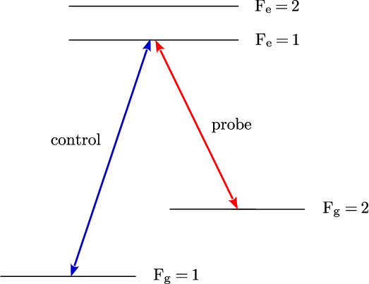
The control laser is on the transition and the probe laser is scanned across the transition.
The levels coupled by the probe and control beams to form the first -type system are shown in Fig. 3. An external magnetic field whose direction (as indicated in the experimental schematic) is parallel to the polarization of the probe beam and orthogonal to that of the control beam.
IV.1.1 Experimental results
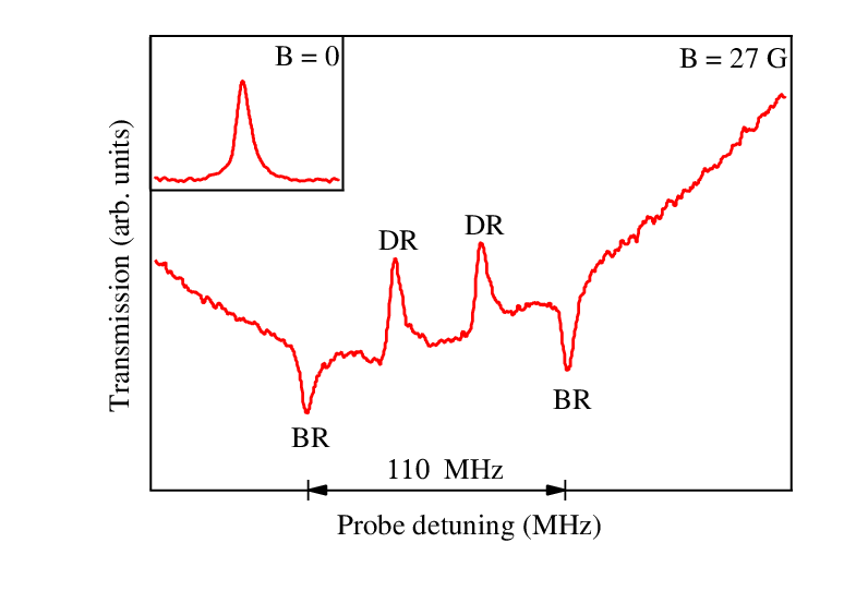
The experimental spectrum is shown in Fig. 4. The curve is obtained with a probe power of and a control power of 13.6 mW. The experiments are done in the presence of a magnetic field of 27 G and the cell is maintained at a temperature of . The curve shows 2 DRs on the inside (corresponding to reduced EIT absorption), and 2 BRs on the outside (corresponding to enhanced EIT absorption). The inset shows that the usual EIT resonance is obtained in the absence of a field.
IV.1.2 Theoretical results
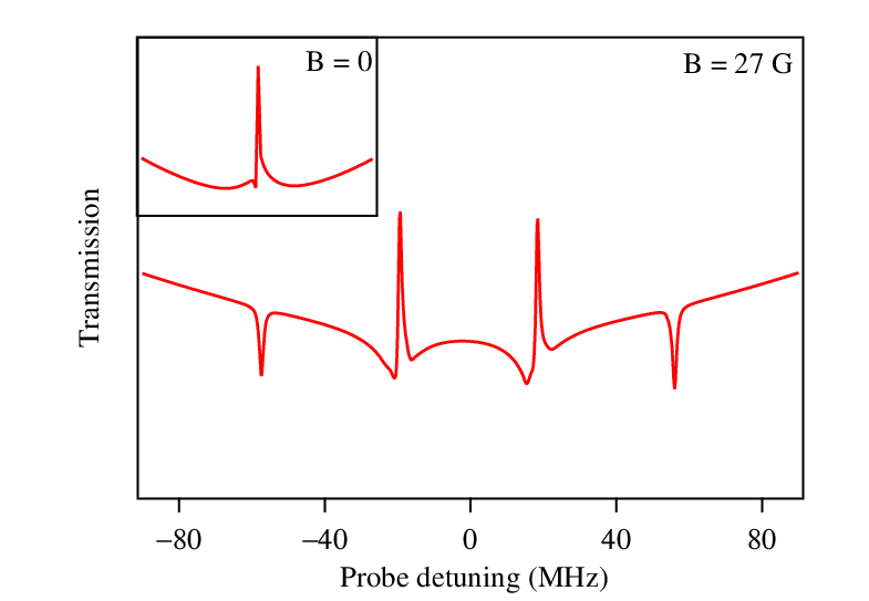
The calculated spectrum is shown in Fig. 5. In this case, the probe beam corresponds to the field, while the control beam corresponds to the field. The calculation is done with probe and control Rabi frequencies corresponding to the powers used in the experiment. The power is related to the Rabi frequency as
where MHz is the natural linewidth of the excited state, is the radius of the beam, and mW/cm2 is the saturation intensity (the intensity at which the transition gets power broadened by a factor of ) of the excited state. The intensity at the center of a Gaussian beam is actually twice as high, but this is taken as some kind of uniform value over the size of the beam. The values of the different relaxation rates are given in the figure caption. The calculation is done with Doppler averaging corresponding to the Maxwell-Boltzmann distribution at a temperature of (absolute temperature of 309 K). The calculation also reproduces the observed fact that a single peak is obtained when the magnetic field is 0, as seen from the inset of the figure.
What is not reproduced by theory in comparison to experiment are the following.
- 1.
The linewidth of the different resonances. This is probably because the Rabi frequency of the two beams are taken to be constant, while in reality they fall off like a Gaussian.
- 2.
IV.1.3 Control over group velocity
This result is important for sub- and super-luminal velocity of light in the medium. In order to see this explicitly, we evaluate the group refractive index for group velocity in terms of the susceptibility . It is given by [22]
where is the velocity of light in vacuum, is the probe frequency, is the number density of atoms, is the dipole matrix element of the probe transition, and is the probe Rabi frequency.
We now plot the group refractive index as a function of probe detuning for the first -type system. The results are shown in Fig. 6. As seen, the index is positive for DRs, which results in sub-luminal propagation of light [23]. BRs have negative index, which results in super-luminal propagation of light [24]. Thus, by tuning from bright to dark resonances, one can switch the system from sub-luminal to super-luminal propagation of light.

IV.2 Second -type system
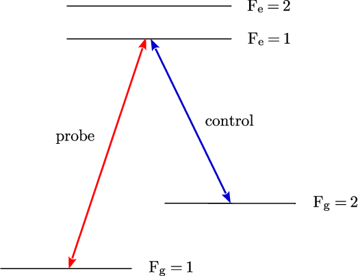
The control laser is on the transition and the probe laser is scanned across the transition.
For the second -type system, the roles of the probe and control beams are interchanged. The levels coupled by the two beams for this system are shown in Fig. 7. A magnetic field with direction similar to the one before is applied.
IV.2.1 Experimental results
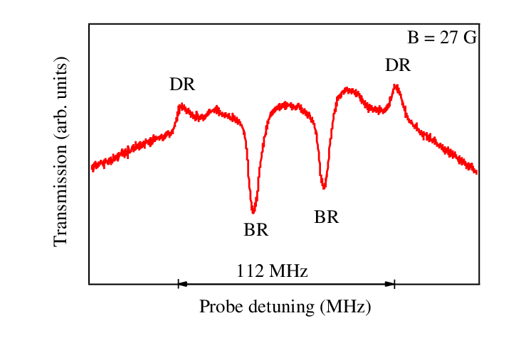
The experimental spectrum shown in Fig. 8, is obtained with a probe power of . This is higher than that for the other system, and is chosen to get an adequate signal-to-noise ratio (SNR). The curve also shows the resonances are inverted, i.e. DRs become BRs and BRs become DRs.
IV.2.2 Theoretical results
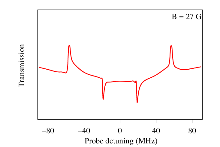
The calculated spectrum is shown in Fig. 9. In this case, the probe beam corresponds to the field, while the control beam corresponds to the field. As in the other case, the calculation is done with probe and control Rabi frequencies corresponding to the ones used in the experiment. The values of the relaxation rates are the same as before, and are given in the figure caption for completeness. Interestingly, it reproduces the experimental observation that the resonances are inverted. As in the other case, the linewidth is narrower and the lineshape is asymmetric, probably for the same reasons as mentioned before.
V Conclusions
In summary, we have studied EIT resonances in a Rb vapor cell with anti-relaxation coating on the walls and in the presence of a 27 G magnetic field. Both bright and dark resonances are obtained as the probe frequency is scanned. The sign of the resonances can be reversed by interchanging the transitions coupled by the probe and control beams. A theoretical explanation based on a density-matrix analysis of the sublevels involved in the transition reproduces the experimental spectra quite well. The different sign of the resonances implies that the same system can be used for both slow and fast propagation of light.
Acknowledgments
A. S. and D. S. are grateful to S. Cartaleva for the ARC glass cell and to E. Mariotti for the PDMS material. V. B. acknowledges financial support from a D. S. Kothari post-doctoral fellowship of the University Grants Commission, India.
References
- [1] E. Arimondo. Coherent population trapping in laser spectroscopy. In E. Wolf, editor, Progress in Optics, volume 35, pages 257–354. Elsevier Science, Amsterdam, 1996.
- [2] Stephen E. Harris. Electromagnetically induced transparency. Phys. Today, 50(7):36–39, 1997.
- [3] Michael Fleischhauer, Atac Imamoglu, and Jonathan P. Marangos. Electromagnetically induced transparency: Optics in coherent media. Rev. Mod. Phys., 77:633–673, Jul 2005.
- [4] C. Goren, A. D. Wilson-Gordon, M. Rosenbluh, and H. Friedmann. Atomic four-level systems. Phys. Rev. A, 69:053818, May 2004.
- [5] L.B. Kong, X.H. Tu, J. Wang, Yifu Zhu, and M.S. Zhan. Sub-doppler spectral resolution in a resonantly driven four-level coherent medium. Opt. Commun., 269(2):362 – 369, 2007.
- [6] Ho-Jung Kim and Han Seb Moon. Wall-induced Ramsey effects on electromagnetically induced absorption. Opt. Express, 20(9):9485–9492, Apr 2012.
- [7] Harish Ravi, Mangesh Bhattarai, Vineet Bharti, and Vasant Natarajan. Polarization-dependent tuning of the Hanle effect in the ground state of Cs. Europhys. Lett., 117(6):63002, 2017.
- [8] R. Wynands and A. Nagel. Precision spectroscopy with coherent dark states. Appl. Phys. B, 68:1–25, 1999.
- [9] D. Budker, W. Gawlik, D. F. Kimball, S. M. Rochester, V. V. Yashchuk, and A. Weis. Resonant nonlinear magneto-optical effects in atoms. Rev. Mod. Phys., 74(4):1153–1201, Nov 2002.
- [10] A. S. Zibrov, A. B. Matsko, O. Kocharovskaya, Y. V. Rostovtsev, G. R. Welch, and M. O. Scully. Transporting and time reversing light via atomic coherence. Phys. Rev. Lett., 88:103601, Feb 2002.
- [11] H. Ravi, M. Bhattarai, Y. D. Abhilash, U. Momeen, and V. Natarajan. Permanent EDM measurement in Cs using nonlinear magneto-optic rotation. Asian Journal of Physics, 25:1093, Nov 2016.
- [12] S. M. Iftiquar and Vasant Natarajan. Line narrowing of electromagnetically induced transparency in Rb with a longitudinal magnetic field. Phys. Rev. A, 79(1):013808, Jan 2009.
- [13] L. Margalit, M. Rosenbluh, and A. D. Wilson-Gordon. Coherent-population-trapping transients induced by a modulated transverse magnetic field. Phys. Rev. A, 88:023827, Aug 2013.
- [14] A. Sargsyan, D. Sarkisyan, Y. Pashayan-Leroy, C. Leroy, S. Cartaleva, A. D. Wilson-Gordon, and M. Auzinsh. Electromagnetically induced transparency resonances inverted in magnetic field. Journal of Experimental and Theoretical Physics, 121(6):966–975, Dec 2015.
- [15] A. Sargsyan, D. Sarkisyan, L. Margalit, and A. D. Wilson-Gordon. Two strongly contrasting -systems in the D1 line of 87Rb in a transverse magnetic field. Journal of Experimental and Theoretical Physics, 122(6):1002–1007, Jun 2016.
- [16] S. M. Rochester. Modeling nonlinear magneto-optical effects in atomic vapors, Ph.D. thesis, 2010.
- [17] M. Bhattarai, V. Bharti, and V. Natarajan. Tuning of the Hanle effect from EIT to EIA using spatially separated probe and control beams. arXiv:1710.04378, Aug 2017.
- [18] A. Sargsyan, C. Leroy, Y. Pashayan-Leroy, R. Mirzoyan, A. Papoyan, and D. Sarkisyan. High contrast d1 line electromagnetically induced transparency in nanometric-thin rubidium vapor cell. Appl. Phys. B, 105(4):767–774, Dec 2011.
- [19] M. Auzinsh, D. Budker, and S. M. Rochester. Optically Polarized Atoms: Understanding Light-Atom Interactions. Oxford University Press, Oxford, United Kingdom, 2010.
- [20] O. S. Mishina, M. Scherman, P. Lombardi, J. Ortalo, D. Felinto, A. S. Sheremet, A. Bramati, D. V. Kupriyanov, J. Laurat, and E. Giacobino. Electromagnetically induced transparency in an inhomogeneously broadened transition with multiple excited levels. Phys. Rev. A, 83:053809, May 2011.
- [21] Vineet Bharti and Ajay Wasan. Influence of multiple excited states on optical properties of an N-type Doppler-broadened system for the D2 line of alkali atoms. J. Phys. B: At. Mol. Opt. Phys., 46(12):125501, 2013.
- [22] Vineet Bharti and Vasant Natarajan. Sub- and super-luminal light propagation using a Rydberg state. Opt. Commun., 392(Supplement C):180 – 184, 2017.
- [23] Lene Vestergaard Hau, S. E. Harris, Zachary Dutton, and Cyrus H. Behroozi. Light speed reduction to 17 metres per second in an ultracold atomic gas. Nature (London), 397:594–598, 1999.
- [24] L. J. Wang, A. Kuzmich, and A. Dogariu. Gain-assisted superluminal light propagation. Nature, 406:277–279, Jul 2000.