MultiMesh Finite Element Methods:
Solving PDEs on Multiple Intersecting Meshes
Abstract
We present a new framework for expressing finite element methods on multiple intersecting meshes: multimesh finite element methods. The framework enables the use of separate meshes to discretize parts of a computational domain that are naturally separate; such as the components of an engine, the domains of a multiphysics problem, or solid bodies interacting under the influence of forces from surrounding fluids or other physical fields. Such multimesh finite element methods are particularly well suited to problems in which the computational domain undergoes large deformations as a result of the relative motion of the separate components of a multi-body system. In the present paper, we formulate the multimesh finite element method for the Poisson equation. Numerical examples demonstrate the optimal order convergence, the numerical robustness of the formulation and implementation in the face of thin intersections and rounding errors, as well as the applicability of the methodology.
In the accompanying paper [1], we analyze the proposed method and prove optimal order convergence and stability.
Keywords:
FEM , unfitted mesh , non-matching mesh , multimesh , CutFEM , Nitsche1 Introduction
Finite element methods (FEM) have been successfully applied to almost all areas of science and engineering where the fundamental model is a partial differential equation or system of partial differential equations, and the applicability and generality of finite element methods are undisputed. This is in part due to the generality of the mathematical formulation, allowing stable numerical schemes of arbitrarily high order accuracy to be formulated for all kinds of PDEs. Another contributing factor is the ability of the finite element method to handle computational domains of complex geometry in both 2D and 3D.
However, the wide applicability of FEM relies on the generation of high-quality computational meshes. For simple domains, mesh generation is not an issue but for complex domains, in particular for time-dependent problems or optimization problems with evolving geometries for which a new mesh may need to be generated many times, mesh generation becomes a limiting factor.
In the current work, we propose a new way to tackle the mesh generation challenge. By allowing the finite element method to be formulated not on a single mesh but on a multitude of meshes, mesh (re)generation is no longer an issue. For example, a rotating propeller may be approximated by a boundary-fitted mesh that rotates freely on top of a fixed background mesh, the interaction of a set of solid bodies may be simulated using a set of individual meshes that may move and intersect freely during the course of a simulation, and the discretization of a composite object may be obtained by superimposing meshes of its individual components. These cases are illustrated in Figure 1.
In short, multimesh finite element methods extend the finite element method to easily handle computational domains composed of parts, where the parts can be either positive or negative (that is, the parts are holes), and where the relative positions and orientations of the parts may change throughout the course of a simulation.

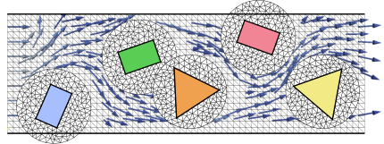
The successful formulation and implementation of multimesh finite element methods rely on three crucial, and challenging, ingredients: (i) consistent finite element formulations that glue together the finite element fields expressed on separate meshes on the common interface, (ii) proper stabilization to ensure stability and optimal order convergence in the presence of very thin intersections between elements from separate meshes, and (iii) efficient and robust computational algorithms and implementation that can quickly and robustly compute the intersections between a multitude of arbitrarily intersecting meshes. The latter part is a particular challenge in the face of rounding errors and floating point arithmetic. It should be noted that critical cases will almost surely appear throughout the course of a simulation involving a large number of relative mesh positions, such as in a time-dependent problem.
1.1 Related work
The multimesh finite element method is based on Nitsche’s method [2], which was initially presented as a method for weakly imposing Dirichlet boundary conditions and later extended to form the basis of discontinuous Galerkin methods [3]. Nitsche’s method is also the basis for CutFEM, the finite element method on cut meshes. The cut finite element was originally proposed in [4, 5] and has since been applied to a range of problems [6, 7, 8, 9]. For an overview, see [10] and [11].
The problem of handling non-matching and multiple meshes is discussed in the literature under many different names, such as fictitious domain, unfitted methods, overset grids and overlapping meshes. Numerous numerical approaches also exists, for example using Lagrange multipliers [12], finite cell methods [13, 14, 15], immersed interface methods [16], the s-version of the finite element method [17, 18] and XFEM [19, 20, 21] to name a few. Discontinuous Galerkin methods have also successfully been used [22, 23, 24, 25], as well as variants using local enrichments [26, 27, 28]. There are also substantial and important works in domain decomposition methods see for example [29, 30] or [31, 32] and the references therein. There are also techniques useful in particular cases, for example in the case of a sliding mesh on top of a fixed background mesh [33, 34].
In cut finite element methods, the finite element solution is represented as a standard (continuous piecewise polynomial) finite element function, either on a fixed background mesh or on a pair of intersecting meshes. Boundary conditions are then imposed weakly either on an intersecting interface, defined for example by a level set function or a discrete surface, or on the interface between two meshes to ensure near continuity of the global finite element field. These boundary conditions are imposed using Nitsche’s method and the method requires the addition of suitable stabilization terms, usually in the form of penalizing jumps in function values or derivatives across interfaces, to ensure stability and optimal order convergence.
The multimesh finite element method is a generalization of CutFEM to general collections of overlapping meshes, where three or more meshes may overlap simultaneously. This imposes new requirements for stabilization and, notably, brings new challenges for robust algorithms and implementation in the face of rounding errors and floating point arithmetic, when tens or hundreds of meshes must be correctly intersected at once, and quadrature rules be computed on the complex shapes resulting from mesh intersections.
The current work is closely related to the work presented in [35, 36] where two overlapping meshes were used to discretize the Stokes problem. The algorithms are similar to those presented in [37] in that axis-aligned bounding boxes (AABB trees) are used for efficient mesh intersection, but different in that we must now consider the intersection of meshes, not just a pair of meshes, and that a new algorithm has been used to compute quadrature rules on cut cells and interfaces. For a detailed exposition of these algorithms and software, we refer to the related work [38].
1.2 Outline
The remainder of this paper is organized as follows. The multimesh finite element method for the Poisson problem is presented in Section 2. The algorithms and implementation of the multimesh finite element method are then briefly discussed in Section 3. Numerical results are presented in Section 4. Finally, conclusions are presented in Section 5.
2 The MultiMesh Finite Element Method
The starting point for the multimesh finite element method is a sequence of standard finite element spaces on meshes, consisting of a single background mesh covering the computational domain and overlapping/intersecting meshes arbitrarily positioned on top of the background mesh. The finite element solution is then expressed as a composite function in the multimesh finite element space and is glued together using Nitsche’s method with appropriate stabilization.
Before we express the method in detail, we here first introduce the concepts and notation for domains, interfaces, meshes, overlaps and function spaces.
2.1 Domains
Let , , be a domain with polygonal boundary (the background domain) and let
| (2.1) |
be subdomains of with polygonal boundaries. We impose an ordering of the domains by saying that is on top of if . For an illustration, see Figure 2. Note that the ordering is not unique as illustrated in Figure 3. We refer to the domains as the predomains. The predomains may or may not intersect each other, but they will intersect the background domain.
We now define a partition of by letting
| (2.2) |
In other words, the domain is the visible part of the predomain ; see Figure 4. Note that by definition, we have have . Also note that some domains may be completely hidden behind domains with a higher index, and thus be empty.
Remark 1
By assumption, the domains are not allowed to intersect the boundary of . This assumption may be too restrictive for some applications, such as for two of the domains shown in the bottom of Figure 1, but we make this assumption for simplicity in the current manuscript. The multimesh finite element method, and indeed also our implementation, support computational domains that extend beyond the boundary of the background mesh.
2.2 Interfaces
Given a sequence of predomains , let
| (2.3) |
In other words, the interface is the visible part of the boundary of ; see Figure 5a. Note that by definition, we have . Also note that does not need to be a closed curve. See also Remark 1.
We may further partition each interface into a set of disjoint interfaces,
| (2.4) |
In other words, the interface is the subset of the visible boundary of the predomain that intersects with the domain , where ; see Figure 5b. Note that some may be empty.
2.3 Meshes
Recall that for a quasi-uniform triangular mesh there exist constants such that for all (see e.g. [39]),
| (2.5) |
where denotes the Lebesgue measure of . Let now be a quasi-uniform premesh on with mesh parameter
| (2.6) |
In other words, the premesh is a mesh of the predomain created by a standard mesh generator; see Figure 6a. We define the global mesh size by .
We further define the active meshes by
| (2.7) |
In other words, the active mesh consists of all (fully or partly) visible elements of the premesh ; see Figure 6b. Placed in the given ordering, the active meshes form the multimesh; see Figure 7b. Note that the active mesh consists of regular (uncut) elements as well as elements which may be partly hidden behind overlapping meshes (the cut elements).
We also define the active domains by
| (2.8) |
In other words, the active domain is the domain defined by the active mesh . Note that typically extends beyond the corresponding domain .
2.4 Overlaps
Given a sequence of active domains , let
| (2.9) |
In other words, the overlap is the hidden part of the active domain . We may further partition each overlap into a set of disjoint overlaps,
| (2.10) |
In other words, the overlap is the hidden part of the elements of the mesh that are hidden below the domain . Since some may be empty, we will make use of the indicator function defined by
| (2.11) |
and let denote the maximum number of non-empty overlaps
| (2.12) |
Note that . For example, in Figure 2, since all three predomains intersect. In Figure 3, and since there are only two intersecting domains.
2.5 Function spaces
Given a sequence of active meshes , let be a continuous piecewise polynomial finite element space on the mesh , the active elements of domain . Note that even if only a part of an element in is visible, the domain extends to the whole elements.
We now define the multimesh finite element space as the direct sum of the individual finite element spaces :
| (2.13) |
An element of is a tuple and the inclusion is defined by the evaluation
| (2.14) |
In other words, is evaluated by evaluating for the highest ranked (topmost) mesh containing the point .
2.6 Finite element method
We may now formulate the multimesh finite element method for the Poisson problem
| (2.15) |
where is a polygonal domain.
Given the construction of the finite element spaces in Section 2.5, the multimesh finite element method for (2.15) is to find such that
| (2.16) |
where
| (2.17) | ||||
| (2.18) | ||||
| (2.19) | ||||
| (2.20) |
Here, and are a stabilization parameters that must be sufficiently large to ensure that the bilinear form is coercive; see [1] for an analysis.
Note that the sum of interface terms extends over the range , since the interface is partitioned into interfaces relative to underlying meshes, whereas the sum of overlap terms extends over the range , since the overlap is partitioned into overlaps relative to overlapping meshes.
We note that the bilinear form contains the standard symmetric Nitsche formulation of (2.15) with jumps and fluxes given pairwise over . The contribution from the bilinear form is a stabilization of the jump in the gradients over . The effect of this term is analyzed in [1]. In short, it ensures that the bilinear form is coercive, which guarantees a unique solution of the problem by the Lax-Milgram theorem [39]. The term also ensures the conditioning of the linear system, which otherwise scales as [40], where is the volume fraction of the smallest cell and is the polynomial order. By including , the condition number scales independently of the volume fraction and only with respect to the mesh size. This is also seen in [10, 38] and similar stabilized methods.
The jump terms on and are given by , where and are the finite element solutions on represented on the active meshes and . On we also define the average normal flux by
| (2.21) |
In the average any convex combination is valid [5]. Note that the finite element method approximates and on all interfaces.
3 Algorithms and Implementation
The multimesh finite element method has been implemented as part of FEniCS [41, 42] and the numerical examples in Section 4 were performed using (a development version of) the 2017.2 release. In this section, we comment briefly on the algorithms and the implementation and refer to the related work [38] for a more detailed exposition.
The evaluation of the integrals appearing in (2.18), (2.19) and (2.20) impose several challenges and rely heavily on the following functionality.
- 1.
Collision detection. For each mesh, compute which elements in the mesh collide with which elements in all other meshes. This step involves computing mesh–mesh collisions.
- 2.
Intersection construction. For each mesh and each colliding element, construct the intersection of the element with the colliding mesh. This step may be reduced to repeated triangulation of simplex–simplex intersections.
- 3.
Quadrature rule construction. For each cut element (not necessarily convex) and each interface, construct a quadrature rule for integration over the cut element or interface.
Efficient construction of quadrature rules is an essential component of a method handling non-matching and multiple meshes. Previous approaches include subtriangulation [37], moment-fitting [43, 44], recursive bisectioning [45, 13], tensor-product based [46], to name a few. One important fact to note in our setting is that curved interfaces can in general be avoided, since the interfaces are completely artificial.
3.1 Collision detection
Given a pair of (pre)meshes and , we compute the collisions between all elements in with all elements in . The collisions are computed by first constructing and then colliding axis-aligned bounding box trees (AABB trees) for the two meshes [47, 48] to find candidate element intersections. The candidate elements are then checked for collision using robust geometric predicates of adaptive precision [49]. The mesh–mesh collision is carried out for each (unordered) pair of premeshes among the meshes.
3.2 Intersection construction
Given a pair of colliding elements and belonging to two different meshes, we compute a subtriangulation of the intersection . Since is convex, the subtriangulation may be computed by a simple Graham scan [50]. When an element collides with more than one element from the same mesh; that is, if collides with , a subtriangulation is created for each pairwise intersection and , etc.
When an element collides with more than one element from multiple meshes; that is, if collides with and , a subtriangulation is first created for the intersection (assuming that ), and then each element in this subtriangulation is further intersected with and new subtriangulations constructed. This procedure guarantees that the only intersections that need to be constructed (triangulated) are pairwise intersections of elements (simplices). This procedure is also the basis for the construction of quadrature rules as described below.
3.3 Quadrature rule construction
Several techniques have been developed for integration over polygonal and polyhedral domains; see, e.g., [51, 44, 43]. However, the construction and representation of general polygonal and polyhedral domains imposes several algorithmic and implementational challenges. Instead, we propose a new approach which, to the authors knowledge, has not been presented before in the literature. We here give a short overview of the basic (and simple) idea and present the details of the algorithm in [38].
We first note that the multimesh method relies on computing integrals over three kinds of domains; these domains are marked as , and in Figure 8. The domain is the hidden part of a cut cell, the domain is the visible part of the cut cell, and is an interface. In 2D the main challenge is the integration over the polygonal domains and and in 3D the challenge is the corresponding integration over polyhedral domains. For the current discussion we thus focus on the integration over these domains and omit the discussion on the integration over (which is simpler).
Consider first the integration over in Figure 8 and note that the domain is the result of repeatedly intersecting a set of triangles. The result of an intersection between two triangles is always a convex polygon. Since a convex polygon can be trivially triangulated (partitioned into triangles), we can easily represent the intersection of two triangles as a union of triangles. We thus first intersect and in Figure 8 and get a set of (two) triangles. We then continue to intersect these triangles with and and the result is a new set of triangles. The quadrature rule over is then easily constructed by summing any standard quadrature rules over the set of triangles.
Consider next the more challenging integration over . If we have only two meshes, we only need to intersect two triangles ( and ). In this case, is given by ; see Figure 9. The key is now to not represent but to instead use the well known inclusion-exclusion principle from combinatorics which states that
| (3.1) |
In other words, a quadrature rule for the union can be constructed by summing the quadrature rules for and and subtracting the quadrature rule for the intersection . It follows that a quadrature rule for the difference is given by
| (3.2) | ||||
| (3.3) | ||||
| (3.4) |
Since now both and can be easily represented as a set of triangles, we can easily compute a quadrature for . Since the inclusion-exclusion principle generalizes to the union of arbitrarily many domains, for example
| (3.5) |
a quadrature rule for the domain can be easily constructed by adding and subtracting the quadrature rules for a set of triangles. The result is a set of quadrature points and weights for , where some of the weights are negative.
4 Numerical Results
In this section, we present a series of numerical results to demonstrate the accuracy and stability of the multimesh finite element formulation presented in Section 2.6, as well as the robustness and generality of the implementation.
4.1 Optimal convergence
We solve the Poisson problem on a discretization of (pre)domains with . The overlapping domains are placed at (uniformly) random positions and scaled to a (uniformly) random size inside such that they do not intersect with the boundary of . We take , where is the polynomial order, and and investigate the convergence for . As a test problem, we consider the analytical solution
| (4.1) |
corresponding to the right-hand side .
Figure 10 shows the random placement of meshes. Due to the fact that the meshes are randomly placed, some domains may be completely covered by other domains in the hierarchy. For this reason, in the case of domains, there are only active domains because one of these domains is completely covered. The same holds for , where only of the domains are visible. For the case with domains, three of the domains are completely covered.
Figure 11 shows the optimal convergence for polynomial orders in the and norms. Detailed convergence rates are summarized in Table 1. As expected, the rate of convergence is in the norm and in the norm.
We note that the errors are of the same order, independently of the number of meshes. In particular, the error for subdomains randomly embedded in the unit square is of the same order as for corresponding to a standard finite element discretization on a single mesh.
A close inspection of Table 1 also reveals that the rate of convergence seems to increase slightly with the number of meshes. The authors believe that this is due to the fact that a larger number of meshes results in a larger number of cut cells and thus an effectively smaller mesh size (more degrees of freedom).
| 0 | 1.9762 | 0.9917 | 2.9965 | 1.9912 | 4.0257 | 3.0044 | 4.9065 | 3.9881 |
|---|---|---|---|---|---|---|---|---|
| 1 | 1.9737 | 0.9911 | 2.9892 | 1.9918 | 4.0235 | 3.0031 | 4.9273 | 3.8062 |
| 2 | 2.1712 | 1.0577 | 3.1886 | 2.0496 | 4.2204 | 3.1060 | 5.0149 | 3.7940 |
| 4 | 2.3019 | 1.1209 | 3.3259 | 2.1110 | 4.4638 | 3.2509 | 5.1200 | 3.9209 |
| 8 | 2.3185 | 1.1522 | 3.3837 | 2.1403 | 4.4083 | 3.2187 | 5.0995 | 3.9484 |
| 16 | 2.3347 | 1.2150 | 3.5285 | 2.1880 | 4.4933 | 3.2945 | 5.4149 | 3.8901 |
| 32 | 2.3142 | 1.2545 | 3.5842 | 2.2190 | 4.7834 | 3.4492 | 5.4546 | 3.9280 |
4.2 Mesh independence
We next investigate the stability of the multimesh finite element method with respect to relative mesh positions, in particular its stability in the presence of thin intersections. We first create a background domain and place on top of this the (pre)domain . We then place domains inside as illustrated in Figure 12 for .
The domains are then step-wise moved closer and closer to the left boundary of at . In particular, the distance between the left boundaries of the meshes is decreased by a factor until the distance to is smaller than machine precision . To be precise, the domains are defined for as follows:
| (4.2) |
where , , and . Note that the shape and size of the domains are kept constant.
For each configuration of the meshes, we compute the multimesh solution of the Poisson problem, using the same exact solution (4.1) as in the previous example. We use elements with and . The linear system is solved using the conjugate gradient method in PETSc [52, 53] with the hypre BoomerAMG preconditioner [54, 55].
We first note that both the and errors in Figure 13 as well as the condition number in Figure 14 (left) increase slightly with the number of meshes . But most importantly, they all remain constant with increasing , i.e., with increasingly thin mesh intersections. This holds even in the extreme regime when approaches to within machine precision.
To investigate the condition number we take the “worst case”, that is, using , fix to and vary . is computed using the quotient of the largest and smallest singular values as found by SLEPc [56, 57]. The condition number for the preconditioned system matrix, , is found from the Krylov solver iterations (the solver is initialized with a random vector and the relative tolerance for convergence is set to ).
The results are found in Figure 14 (right) and show that . The last four points have slope why we believe that in the limit . This is the result obtained by the analysis presented in [1] and is the usual result for second-order elliptic problems. The results for seem to be dependent a little on , and the actual values are somewhat large. More work on how to effectively precondition these systems are thus of great interest.
4.3 Electrostatic interaction of charged bodies
As a challenging application of the multimesh formulation and implementation, we model a collection of charged rigid bodies interacting under the influence of the electric field generated by the charges. For simplicity, we set all physical units and material parameters – masses, mass densities, the electric permittivity, etc. – to .
Consider three disjoint domains , and in . The charge density is inside each of the three domains and outside. In other words,
| (4.3) |
The electric potential is then given by the solution of the Poisson problem
| (4.4) | ||||||
| (4.5) |
and the electric field is .
The electric field gives rise to a force and a torque on each domain where is the center of mass of the domain . The electric field and the torque generate an acceleration of the center of mass and an angular acceleration around the center of mass for each domain. The three domains are enclosed inside a square domain and contact with the boundary of the box is modeled as a fully elastic collision, i.e., by reversing the normal velocity and angular momentum.
We simulate the electrostatic interaction of the three bodies by enclosing each domain in a surrounding boundary-fitted mesh and superimposing the three meshes onto a fixed background mesh. The background mesh is made large to model the Dirichlet boundary condition at infinity, and adaptively refined in the interior of the box enclosing the charged bodies, as shown in Figure 15. We thus have premeshes, with mesh being the background mesh, and , , being the three overlapping meshes. For each overlapping premesh , we divide the elements into two subdomains (using markers) to indicate the interior containing the charge and the exterior where the charge is zero.
In each time step, the electric potential is computed using the multimesh discretization of the Poisson problem (4.4)–(4.5). For sake of variation, we use the alternative stabilization term
| (4.6) |
with ; see [1] for a discussion. The interior penalty parameter is chosen to be .
Once the electric potential has been computed, the electric field is computed by projecting the negative gradient of the potential to a vector-valued piecewise linear multimesh space. For the projection, we use a similar stabilized variational formulation as for the Poisson problem:
| (4.7) |
with and . From the electric field, we may then compute the forces and torques on the three rigid bodies , and .
The dynamics of the rigid bodies is computed using the symplectic Euler scheme; i.e., by first updating the velocities and angular velocities and then updating the positions and rotation angles using the newly computed velocities and angular velocities.


The electric charge distribution gives rise to an electric force repelling the three rigid bodies, which then bounce against the boundaries of the enclosing rigid box for 1000 time steps of size (). In each time step, new intersections and quadrature points are computed for the multimesh discretization on the current configuration of the three meshes on top of the fixed background mesh. The computed electric potential and electric field are shown in Figures 16 and 17. Throughout the 1000 time steps of the simulation, the electric potential and electric field exhibit a smooth transition across the boundaries of the four meshes, which demonstrates the stability of the finite element formulation and the robustness of the implementation. An animation of the time evolution of the electric potential and the dynamics of the rigid bodies is available on YouTube at https://youtu.be/jBINWmALrps


5 Conclusions and Future Work
We have presented a general framework for discretization of partial differential equations posed on a domain defined by an arbitrary number of intersecting meshes. The framework has been formulated in the context of the Poisson problem, and numerical results presented to support the optimal order convergence and demonstrate the capabilities of the algorithms and implementation. In the accompanying paper [1], we return to the analysis of the proposed finite element formulation and present optimal order estimates of errors and condition numbers.
In related work [38], the algorithms and implementation are discussed in more detail. Ongoing and future work by the authors are focused on optimizations and generalizations of the presented formulation, and algorithms and software to enable application to more demanding problems, in particular to multiphysics problems posed on complex and evolving geometries in 3D. The proposed technique for constructing the quadrature rules is dimension independent. However, the collision detection and intersection construction depend on the geometrical (and topological) dimension. The geometric predicate library [49] provides routines in both 2D and 3D. The intersection construction is currently done in a case-by-case basis and is work in progress. An application to shape optimization is presented in [58].
6 Acknowledgements
August Johansson was supported by The Research Council of Norway through a Centres of Excellence grant to the Center for Biomedical Computing at Simula Research Laboratory, project number 179578, as well as by the Research Council of Norway through the FRIPRO Program at Simula Research Laboratory, project number 25123. Benjamin Kehlet was supported by The Research Council of Norway through a Centres of Excellence grant to the Center for Biomedical Computing at Simula Research Laboratory, project number 179578. Mats G. Larson was supported in part by the Swedish Foundation for Strategic Research Grant No. AM13-0029, the Swedish Research Council Grants Nos. 2013-4708, 2017-03911, and the Swedish Research Programme Essence. Anders Logg was supported by the Swedish Research Council Grant No. 2014-6093.
References
- [1] A. Johansson, B. Kehlet, M. G. Larson, A. Logg, MultiMesh Finite Element Methods: Analysis, Submitted. https://arxiv.org/abs/1804.06455.
- [2] J. Nitsche, Über ein Variationsprinzip zur Lösung von Dirichlet-Problemen bei Verwendung von Teilräumen, die keinen Randbedingungen unterworfen sind, in: Abhandlungen aus dem Mathematischen Seminar der Universität Hamburg, Vol. 36, Springer, 1971, pp. 9–15. doi:10.1007/BF02995904.
- [3] D. N. Arnold, An interior penalty finite element method with discontinuous elements, SIAM J. Numer. Anal. 19 (4) (1982) 742–760. doi:10.1137/0719052.
- [4] A. Hansbo, P. Hansbo, An unfitted finite element method, based on Nitsche’s method, for elliptic interface problems, Comput. Method. Appl. M. 191 (47-48) (2002) 5537 – 5552. doi:10.1016/S0045-7825(02)00524-8.
- [5] A. Hansbo, P. Hansbo, M. G. Larson, A finite element method on composite grids based on Nitsche’s method, ESAIM-Math. Model. Num. 37 (3) (2003) 495–514. doi:10.1051/m2an:2003039.
- [6] E. Burman, P. Hansbo, A unified stabilized method for Stokes’ and Darcy’s equations, J. Comput. Appl. Math. 198 (1) (2007) 35–51. doi:10.1016/j.cam.2005.11.022.
- [7] E. Burman, M. A. Fernández, Stabilized explicit coupling for fluid-structure interaction using Nitsche’s method, C. R. Math. Acad. Sci. Paris 345 (8) (2007) 467–472. doi:10.1016/j.crma.2007.09.010.
- [8] R. Becker, E. Burman, P. Hansbo, A Nitsche extended finite element method for incompressible elasticity with discontinuous modulus of elasticity, Comp. Methods Appl. Mech. Engrg. 198 (41) (2009) 3352–3360. doi:10.1016/j.cma.2009.06.017.
- [9] A. Massing, M. G. Larson, A. Logg, M. E. Rognes, A nitsche-based cut finite element method for a fluid–structure interaction problem, Communications in Applied Mathematics and Computational Science 10. doi:10.2140/camcos.2015.10.97.
- [10] E. Burman, S. Claus, P. Hansbo, M. G. Larson, A. Massing, CutFEM: Discretizing geometry and partial differential equations, International Journal for Numerical Methods in Engineering 104 (7) (2015) 472–501. doi:10.1002/nme.4823.
- [11] S. P. A. Bordas, E. Burman, M. G. Larson, M. A. Olshanskii, Geometrically Unfitted Finite Element Methods and Applications, Vol. 121 of Lecture Notes in Computational Science and Engineering, Springer International Publishing, 2017. doi:10.1007/978-3-319-71431-8.
- [12] E. Burman, P. Hansbo, Fictitious domain finite element methods using cut elements: I. a stabilized lagrange multiplier method, Computer Methods in Applied Mechanics and Engineering 199 (41) (2010) 2680 – 2686. doi:10.1016/j.cma.2010.05.011.
- [13] D. Schillinger, M. Ruess, The finite cell method: A review in the context of higher-order structural analysis of cad and image-based geometric models, Archives of Computational Methods in Engineering 22 (3) (2015) 391–455. doi:10.1007/s11831-014-9115-y.
- [14] A. Düster, J. Parvizian, Z. Yang, E. Rank, The finite cell method for three-dimensional problems of solid mechanics, Computer Methods in Applied Mechanics and Engineering 197 (45) (2008) 3768 – 3782. doi:10.1016/j.cma.2008.02.036.
- [15] J. Parvizian, A. Düster, E. Rank, Finite cell method, Computational Mechanics 41 (1) (2007) 121–133. doi:10.1007/s00466-007-0173-y.
- [16] Z. Li, The immersed interface method using a finite element formulation, Applied Numerical Mathematics 27 (3) (1998) 253 – 267. doi:10.1016/S0168-9274(98)00015-4.
- [17] J. Fish, The s-version of the finite element method, Computers & Structures 43 (3) (1992) 539 – 547. doi:10.1016/0045-7949(92)90287-A.
- [18] J. Fish, S. Markolefas, R. Guttal, P. Nayak, On adaptive multilevel superposition of finite element meshes for linear elastostatics, Applied Numerical Mathematics 14 (1) (1994) 135 – 164. doi:10.1016/0168-9274(94)90023-X.
- [19] T.-P. Fries, T. Belytschko, The extended/generalized finite element method: An overview of the method and its applications, International Journal for Numerical Methods in Engineering 84 (3) (2010) 253–304. doi:10.1002/nme.2914.
- [20] J. Chessa, P. Smolinski, T. Belytschko, The extended finite element method (xfem) for solidification problems, International Journal for Numerical Methods in Engineering 53 (8) (2002) 1959–1977. doi:10.1002/nme.386.
- [21] C. Lehrenfeld, High order unfitted finite element methods on level set domains using isoparametric mappings, Computer Methods in Applied Mechanics and Engineering 300 (2016) 716 – 733. doi:10.1016/j.cma.2015.12.005.
- [22] P. Bastian, C. Engwer, An unfitted finite element method using discontinuous Galerkin, International Journal for Numerical Methods in Engineering 79 (12) (2009) 1557–1576. doi:10.1002/nme.2631.
- [23] A. Johansson, M. G. Larson, A high order discontinuous Galerkin Nitsche method for elliptic problems with fictitious boundary, Numer. Math. 123 (4) (2013) 607–628. doi:10.1007/s00211-012-0497-1.
- [24] R. Saye, Implicit mesh discontinuous Galerkin methods and interfacial gauge methods for high-order accurate interface dynamics, with applications to surface tension dynamics, rigid body fluid-structure interaction, and free surface flow: Part i, Journal of Computational Physics 344 (Supplement C) (2017) 647 – 682. doi:10.1016/j.jcp.2017.04.076.
- [25] R. Saye, Implicit mesh discontinuous Galerkin methods and interfacial gauge methods for high-order accurate interface dynamics, with applications to surface tension dynamics, rigid body fluid-structure interaction, and free surface flow: Part ii, Journal of Computational Physics 344 (Supplement C) (2017) 683 – 723. doi:10.1016/j.jcp.2017.05.003.
- [26] R. Bouclier, J.-C. Passieux, M. Salaün, Local enrichment of nurbs patches using a non-intrusive coupling strategy: Geometric details, local refinement, inclusion, fracture, Computer Methods in Applied Mechanics and Engineering 300 (2016) 1 – 26. doi:10.1016/j.cma.2015.11.007.
- [27] N. Zander, T. Bog, S. Kollmannsberger, D. Schillinger, E. Rank, Multi-level hp-adaptivity: high-order mesh adaptivity without the difficulties of constraining hanging nodes, Computational Mechanics 55 (3) (2015) 499–517.
- [28] D. Schillinger, L. Dedè, M. A. Scott, J. A. Evans, M. J. Borden, E. Rank, T. J. Hughes, An isogeometric design-through-analysis methodology based on adaptive hierarchical refinement of nurbs, immersed boundary methods, and t-spline cad surfaces, Computer Methods in Applied Mechanics and Engineering 249-252 (2012) 116 – 150, higher Order Finite Element and Isogeometric Methods. doi:10.1016/j.cma.2012.03.017.
- [29] E. Rank, Adaptive remeshing and h-p domain decomposition, Computer Methods in Applied Mechanics and Engineering 101 (1) (1992) 299 – 313. doi:10.1016/0045-7825(92)90027-H.
- [30] Becker, Roland, Hansbo, Peter, Stenberg, Rolf, A finite element method for domain decomposition with non-matching grids, ESAIM: M2AN 37 (2) (2003) 209–225. doi:10.1051/m2an:2003023.
- [31] D. Appelö, J. W. Banks, W. D. Henshaw, D. W. Schwendeman, Numerical methods for solid mechanics on overlapping grids: Linear elasticity, Journal of Computational Physics 231 (18) (2012) 6012 – 6050. doi:10.1016/j.jcp.2012.04.008.
- [32] W. D. Henshaw, D. W. Schwendeman, Parallel computation of three-dimensional flows using overlapping grids with adaptive mesh refinement, J. Comput. Phys. 227 (16) (2008) 7469–7502. doi:10.1016/j.jcp.2008.04.033.
- [33] M. Behr, T. Tezduyar, The shear-slip mesh update method, Computer Methods in Applied Mechanics and Engineering 174 (3) (1999) 261 – 274. doi:https://doi.org/10.1016/S0045-7825(98)00299-0.
- [34] B. Y., K. A., D. X., Y. J., Novel structural modeling and mesh moving techniques for advanced fluid–structure interaction simulation of wind turbines, International Journal for Numerical Methods in Engineering 102 (3-4) 766–783. doi:10.1002/nme.4738.
- [35] A. Massing, M. G. Larson, A. Logg, M. E. Rognes, A stabilized Nitsche overlapping mesh method for the Stokes problem, Numerische Mathematik (2014) 1–29doi:10.1007/s00211-013-0603-z.
- [36] A. Johansson, M. G. Larson, A. Logg, High order cut finite element methods for the Stokes problem, Advanced Modeling and Simulation in Engineering Sciences 2 (1) (2015) 1–23. doi:10.1186/s40323-015-0043-7.
- [37] A. Massing, M. G. Larson, A. Logg, Efficient implementation of finite element methods on non-matching and overlapping meshes in 3d, SIAM Journal on Scientific Computing 35 (1) (2013) C23–C47. doi:10.1137/11085949X.
- [38] A. Johansson, B. Kehlet, A. Logg, Construction of quadrature rules on general polygonal and polyhedral domains in cut finite element methods, In preparation.
- [39] S. C. Brenner, L. R. Scott, The Mathematical Theory of Finite Element Methods, Springer, New York, 2008. doi:10.1007/978-0-387-75934-0.
- [40] F. de Prenter, C. Verhoosel, G. van Zwieten, E. van Brummelen, Condition number analysis and preconditioning of the finite cell method, Computer Methods in Applied Mechanics and Engineering 316 (2017) 297 – 327, special Issue on Isogeometric Analysis: Progress and Challenges. doi:10.1016/j.cma.2016.07.006.
- [41] A. Logg, K.-A. Mardal, G. N. Wells, et al., Automated Solution of Differential Equations by the Finite Element Method, Springer, 2012. doi:10.1007/978-3-642-23099-8.
- [42] M. S. Alnæs, J. Blechta, J. Hake, A. Johansson, B. Kehlet, A. Logg, C. Richardson, J. Ring, M. E. Rognes, G. N. Wells, The fenics project version 1.5, Archive of Numerical Software 3 (100). doi:10.11588/ans.2015.100.20553.
- [43] Y. Sudhakar, W. A. Wall, Quadrature schemes for arbitrary convex/concave volumes and integration of weak form in enriched partition of unity methods, Computer Methods in Applied Mechanics and Engineering 258 (Supplement C) (2013) 39 – 54. doi:10.1016/j.cma.2013.01.007.
- [44] B. Müller, F. Kummer, M. Oberlack, Highly accurate surface and volume integration on implicit domains by means of moment-fitting, International Journal for Numerical Methods in Engineering 96 (8) (2013) 512–528. doi:10.1002/nme.4569.
- [45] C. Verhoosel, G. van Zwieten, B. van Rietbergen, R. de Borst, Image-based goal-oriented adaptive isogeometric analysis with application to the micro-mechanical modeling of trabecular bone, Computer Methods in Applied Mechanics and Engineering 284 (2015) 138 – 164, isogeometric Analysis Special Issue. doi:10.1016/j.cma.2014.07.009.
- [46] R. Saye, High-order quadrature methods for implicitly defined surfaces and volumes in hyperrectangles, SIAM Journal on Scientific Computing 37 (2) (2015) A993–A1019. doi:10.1137/140966290.
- [47] T. Akenine-Möller, E. Haines, N. Hoffman, Real-Time Rendering 3rd Edition, A. K. Peters, Ltd., Natick, MA, USA, 2008.
- [48] C. Ericson, Real-Time Collision Detection, CRC Press, Inc., Boca Raton, FL, USA, 2004.
- [49] J. R. Shewchuk, Adaptive Precision Floating-Point Arithmetic and Fast Robust Geometric Predicates, Discrete & Computational Geometry 18 (3) (1997) 305–363. doi:10.1007/PL00009321.
- [50] R. L. Graham, An efficient algorithm for determining the convex hull of a finite planar set, Information Processing Letters 1 (4) (1972) 132 – 133. doi:10.1016/0020-0190(72)90045-2.
- [51] S. E. Mousavi, H. Xiao, N. Sukumar, Generalized gaussian quadrature rules on arbitrary polygons, International Journal for Numerical Methods in Engineering 82 (1) (2010) 99–113. doi:10.1002/nme.2759.
- [52] S. Balay, S. Abhyankar, M. F. Adams, J. Brown, P. Brune, K. Buschelman, L. Dalcin, V. Eijkhout, W. D. Gropp, D. Kaushik, M. G. Knepley, L. C. McInnes, K. Rupp, B. F. Smith, S. Zampini, H. Zhang, H. Zhang, PETSc users manual, Tech. Rep. ANL-95/11 - Revision 3.8, Argonne National Laboratory (2017).
- [53] S. Balay, W. D. Gropp, L. C. McInnes, B. F. Smith, Efficient management of parallelism in object oriented numerical software libraries, in: E. Arge, A. M. Bruaset, H. P. Langtangen (Eds.), Modern Software Tools in Scientific Computing, Birkhäuser Press, 1997, pp. 163–202. doi:10.1007/978-1-4612-1986-6_8.
- [54] V. E. Henson, U. M. Yang, Boomeramg: A parallel algebraic multigrid solver and preconditioner, Appl. Numer. Math. 41 (2002) 155–177. doi:10.1016/S0168-9274(01)00115-5.
- [55] Lawrence Livermore National Laboratory, hypre: High Performance Preconditioners, http://www.llnl.gov/CASC/hypre/, accessed 2018-03-14.
- [56] V. Hernandez, J. E. Roman, V. Vidal, SLEPc: A scalable and flexible toolkit for the solution of eigenvalue problems, ACM Trans. Math. Software 31 (3) (2005) 351–362. doi:10.1145/1089014.1089019.
- [57] J. E. Roman, C. Campos, E. Romero, A. Tomas, SLEPc users manual, Tech. Rep. DSIC-II/24/02 - Revision 3.8, D. Sistemes Informàtics i Computació, Universitat Politècnica de València (2017).
- [58] J. S. Dokken, S. W. Funke, A. Johansson, S. Schmidt, Shape optimization on multiple meshes, In preparation.