Origin of chaos near three-dimensional quantum vortices:
A general Bohmian theory

Consider a 3-d quantum system with wavefunction $\Psi(x,y,z,t)$, at the time $t$, where $(x,y,z)$ are Cartesian space co-ordinates. The quantum current is given by $\mathbf{j}=\frac{\hbar}{2mi}(\Psi^{*}\nabla\Psi-\Psi\nabla\Psi^{*})$ ($\hbar=$Planck’s constant, $m=$ the particle mass, $\hbar=m=1$ in the sequel). The quantum current can be traced by a swarm of ‘Bohmian’ trajectories defined via the flow $\mathbf{v}=\mathbf{j}/|\Psi|^{2}$. These equations of motion take the generic form

$$\frac{dx}{dt}=f_{x}(x,y,z,t),\,\,\,\frac{dy}{dt}=f_{y}(x,y,z,t),\,\,\,\frac{dz}{dt}=f_{z}(x,y,z,t)~~.$$

(1)

Eqs.(1) constitute a non-autonomous 3-d dynamical system. Numerical investigations in various systems of the form (1) have revealed the typical existence of chaotic trajectories (see, for example [27, 29, 45]. Our purpose is to explain the dynamical origin of the trajectories’ chaotic behavior. To this end, it proves crucial to focus on the structure of the flow induced by Eqs.(1) near loci in space where $\Psi(x,y,z,t)=0$. These loci are the ‘nodal lines’ of the wavefunction $\Psi$.

We invoke the following two approximations, further specified in subsequent sections:

i) Under an appropriate ‘adiabatic’ condition (see subsection II.5), the flow (1) in a neighborhood of every point along a nodal line, and within a given time interval, can be approximated as nearly autonomous in a set of variables $(u,v,w)$, found after a linear transformation ${\cal L}:(x,y,z)\rightarrow(u,v,w)$. The variables $(u,v,w)$ correspond physically to co-ordinates locally attached to and co-moving with each separate nodal point along a nodal line.

ii) One can use the above co-ordinates in order to construct a new dynamical system of the form:

$$\frac{dU}{d\tau}=F_{U}(U,V,S),~~\frac{dV}{d\tau}=F_{V}(U,V,S),~~\frac{dS}{d\tau}=F_{S}(U,V,S)$$

(2)

where the variables $(U,V,S)$ are provided by a transformation

$$(U,V,S)=(u,v,w)+{\cal NL}(u,v,w)$$

(3)

${\cal NL}(u,v,w)$ being a small nonlinear correction to the identity. The new time $\tau$ corresponds to a suitably defined re-parametrization of the original time $t$.

Using the above approximations, we deduce the following, which is the main result of the present paper: We show that the equations of motion (2) admit as solution an invariant continuous family of hyperbolic points, which, together, form a normally hyperbolic ‘X-line’. Furthermore, the stable and unstable manifolds of the X-line connect with the associated nodal line through a family of spirals, forming a 3-d vortex. This we call the ‘3-d structure of nodal point - X-point complexes’. The geometric structure of these manifolds serves to explain the hyperbolic scattering of nearby trajectories, i.e., the appearance of chaos near 3-d quantum vortices. In particular, it is the dynamics close to the X-line, rather than close to the nodal line, which is responsible for chaos. This latter fact is substantiated with numerical experiments in section III.

The complete construction of the transformation (3), as well as the Eqs.(2), is given in Appendix I. Most features of these equations can be approximated by a local construction, which yields equations of motion around only one nodal point along a nodal line. We now focus on the latter construction, which is similar as the one introduced in [33] for 2-d systems.

Let $\Psi_{R}(x,y,z,t)=\Re(\Psi(x,y,z,t))$, $\Psi_{I}(x,y,z,t)=\Im(\Psi(x,y,z,t))$. We assume that, at fixed time $t$, the $2\times 3$ set of equations

$$\Psi_{R}(x,y,z,t)=0,~~~\Psi_{I}(x,y,z,t)=0$$

(4)

admits solutions lying in one or more curves in the space $(x,y,z)$. We call such curves the ‘nodal lines’ of the wavefunction $\Psi$ at the time $t$.

Depending on the wavefunction under study, the shape of nodal lines at a given time $t$ can be quite complex, as it can be composed of different branches, possibly forming loops or extending to infinity. On the other hand, it is possible to introduce a continuous parametrization of one nodal line in every open segment of it. To this end, let O be an arbitrary point along a nodal line not belonging to its boundary (we call O the ‘origin’). In an open neighborhood ${\cal V}_{0}$ of $O$, we define $s$ to be the length parameter along the curve, starting from O and with sign indicating the direction of inscription of the line with respect to O. For every point of the nodal line $(x_{0},y_{0},z_{0})$ belonging to ${\cal V}_{0}$ we can then assign a unique value of $s$, thus defining the continuous and smooth functions $x_{0}(s),y_{0}(s),z_{0}(s)$.

Setting $\Psi=\Psi_{R}+i\Psi_{I}$, the Bohmian equations of motion in the inertial frame read (with $m=\hbar=1$):

$$\mathbf{v}=\dot{\mathbf{r}}=\frac{\Psi_{R}\nabla\Psi_{I}-\Psi_{I}\nabla\Psi_{R}}{\Psi_{R}^{2}+\Psi_{I}^{2}}.$$

(5)

Since $\Psi_{R}(x_{0}(s),y_{0}(s),z_{0}(s),t)=\Psi_{I}(x_{0}(s),y_{0}(s),z_{0}(s),t)=0$ one has

$$\frac{d\Psi_{R}}{ds}=\nabla\Psi_{R}\cdot\frac{d\mathbf{r_{0}}}{ds}=0,\,\,\,\,\frac{d\Psi_{I}}{ds}=\nabla\Psi_{I}\cdot\frac{d\mathbf{r_{0}}}{ds}=0$$

(6)

and, hence, $\nabla\Psi_{R}\perp d\mathbf{r_{0}}/ds$, $\nabla\Psi_{I}\perp d\mathbf{r_{0}}/ds$ at all points $\mathbf{r_{0}}\equiv(x_{0},y_{0},z_{0})$. Then, by Eq.(5) we deduce that the Bohmian velocity field tends to become normal to the nodal curve as we tend towards any point on this curve. The plane normal to a nodal curve at one of its nodal points is called the ‘F-plane’ associated with the nodal point (see [29]).

Assuming the wavefunction to be continuous and with continuous derivatives in ${\cal V}_{0}$ at all times between $t$ and $t+\Delta t$, where $\Delta t$ is a small time interval, Eqs.(4) imply that the nodal line evolves smoothly in time within ${\cal V}_{0}$. In particular, let ${\cal F}_{\mathbf{r}_{0},t}$ be the F-plane associated with the nodal point $\mathbf{r}_{0}$ at the time $t$, and $\mathbf{r}_{0}(t^{\prime})$ be the point where the nodal line at a later time $t^{\prime}$ intersects the same F-plane ${\cal F}_{\mathbf{r}_{0},t}$, for all $t^{\prime}$ with $t\leq t^{\prime}\leq t+\Delta t$. We define the velocity $\mathbf{V}_{0}$ of the nodal point $\mathbf{r}_{0}$ at the time $t$ as

$$\mathbf{V}_{0}(t)=\lim_{t^{\prime}\rightarrow t}\frac{\mathbf{r}_{0}(t^{\prime})-\mathbf{r}_{0}(t)}{t^{\prime}-t}~~.$$

(7)

Clearly, the velocity vector $\mathbf{V}_{0}(t)$ belongs to ${\cal F}_{\mathbf{r}_{0},t}$, thus it is also perpendicular to the nodal line.

We note here that, as it will be discussed below, ‘X-lines’ necessarily appear only when we consider the quantum flow around time-varying nodal lines. Similarly to the 2-d case (see [32, 33]), in order to describe this phenomenon we must consider the form of the quantum flow in a co-ordinate frame co-moving with the nodal line. In turn, this requires assigning a value of the velocity to every point along the nodal line. However, contrary to the 2-d case, in the 3-d case such assignment cannot be done unambiguously on the sole basis of the shape evolution of the nodal line at nearby times, since there are infinitely many ways to continuously map each point of the nodal line, at time $t$, to a point on the deformation of the same nodal line at a later time $t^{\prime}>t$. Using the intersection of the nodal line with the F-plane ${\cal F}_{\mathbf{r}_{0},t}$ allows to bypass this ambiguity. ¹¹ 1 One may also remark that the Bohmian equations (5) cannot be used directly to define $\mathbf{V}_{0}(t)$, since the r.h.s. of these equations are singular at $\mathbf{r}=\mathbf{r}_{0}$ at the time $t$.

Let $\mathbf{r}_{0}=(x_{0},y_{0},z_{0})$ be a particular nodal point at the time $t=t_{0}$. We now consider a coordinate change $(x,y,z)\rightarrow(u,v,w)$ such that: i) $(x_{0},y_{0},z_{0})\rightarrow(0,0,0)$, i.e. the node is at the origin, ii) the new co-ordinates are such that the w-axis is tangent to the nodal line at the point $(x_{0},y_{0},z_{0})$, while the $u$ and $v$ are directions in the associated F-plane defined via a pre-selected geometric rule. For example, if $\mathbf{t}$, $\mathbf{n}$, $\mathbf{b}$ are the tangent, normal and bi-normal unitary vectors of the nodal line at $\mathbf{r}_{0}$, for an arbitrary point $\mathbf{r}\equiv(x,y,z)$ we define the transformation (Fig. 2):

$$u=\mathbf{\Delta r}\cdot\mathbf{n},~~v=\mathbf{\Delta r}\cdot\mathbf{b},~~w=\mathbf{\Delta r}\cdot\mathbf{t}$$

(8)

where $\mathbf{\Delta r}=\mathbf{r}-\mathbf{r}_{0}$. Since Eqs.(8) become singular at points $\mathbf{r}_{0}$ where the curvature of the nodal line becomes zero, we can use, alternatively, the transformation:

$$\begin{pmatrix}u\\ v\\ w\end{pmatrix}=\begin{bmatrix}\sin{\phi_{m}}&-\cos{\phi_{m}}&0\\ \cos{\theta_{m}}\cos{\phi_{m}}&\cos{\theta_{m}}\sin{\phi_{m}}&-\sin{\theta_{m}}\\ \sin{\theta_{m}}\cos{\phi_{m}}&\sin{\theta_{m}}\sin{\phi_{m}}&\cos{\theta_{m}}\end{bmatrix}\begin{pmatrix}x-x_{0}\\ y-y_{0}\\ z-z_{0}\end{pmatrix}$$

(9)

with

		$\displaystyle\phi_{m}=\arctan(t_{y}/t_{x})$		(10)
		$\displaystyle\theta_{m}=\arccos(t_{z}/|t|)$		(11)

where $\mathbf{t}=(t_{x},t_{y},t_{z})$. Equations (9) become singular whenever $\mathbf{t}$ becomes parallel to the z-axis. In numerical simulations we use both (8) and (9), ensuring to properly deal with the corresponding singularities.

Expressing $\Psi$ in the new co-ordinates $\Psi\equiv\Psi(u,v,w,t)$, Eqs.(4) and (6) take the form

$$\Psi(0,0,0,t=t_{0})=0,~~~\frac{\partial\Psi}{\partial w}\Bigg|_{u=0,v=0,w=0,t=t_{0}}=0~~$$

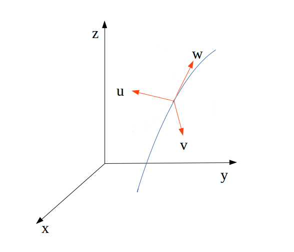
Then, Taylor-expanding $\Psi$ around the origin (the nodal point) and up to terms of second degree in the variables $u,v,w$ yields

	$\displaystyle\Psi$	$\displaystyle=$	$\displaystyle a_{000}+(a_{100}+ib_{100})u+(a_{010}+ib_{010})v+(a_{200}+ib_{200})u^{2}+(a_{020}+ib_{020})v^{2}$		(12)
		$\displaystyle+$	$\displaystyle(a_{002}+ib_{002})w^{2}+(a_{110}+ib_{110})uv+(a_{101}+ib_{101})uw+(a_{001}+ib_{001})vw+\ldots$

with real time-dependent coefficients $a_{ijk}(t)$, $b_{ijk}(t)$, $i,j,k=0,1,\dots$. One has $a_{000}(t_{0})=0$. As in the corresponding analysis in the 2-d case (see [33]), we now consider a frame of reference centered at the nodal point $\mathbf{r}_{0}$ and moving with uniform velocity $(V_{u},V_{v},V_{w})$ equal to the instantaneous velocity $\mathbf{V}_{0}$ of the nodal point defined in Eq.(7). Setting $G=\Psi_{R}^{2}+\Psi_{I}^{2}=(a_{100}u+a_{010}v)^{2}+(b_{100}u+b_{010}v)^{2}+\dots$, the equations of motion in the above frame read

	$\displaystyle\frac{du}{dt}$	$\displaystyle=$	$\displaystyle\frac{1}{G}\bigg[\Big(\frac{\partial\Psi_{I}}{\partial u}\Psi_{R}-\frac{\partial\Psi_{R}}{\partial u}\Psi_{I}\Big)-V_{u}G\bigg]$
	$\displaystyle\frac{dv}{dt}$	$\displaystyle=$	$\displaystyle\frac{1}{G}\bigg[\Big(\frac{\partial\Psi_{I}}{\partial v}\Psi_{R}-\frac{\partial\Psi_{R}}{\partial v}\Psi_{I}\Big)-V_{v}G\bigg]$		(13)
	$\displaystyle\frac{dw}{dt}$	$\displaystyle=$	$\displaystyle\frac{1}{G}\bigg[\Big(\frac{\partial\Psi_{I}}{\partial w}\Psi_{R}-\frac{\partial\Psi_{R}}{\partial w}\Psi_{I}\Big)-V_{w}G\bigg]~~.$

We have $V_{w}=0$, since, by definition, the velocity $\mathbf{V}_{0}$ is orthogonal to the nodal line. We also note that the r.h.s. of Eqs.(13) depends explicitly on time through the time dependence of the wavefunction $\Psi$.

Due to Eq.(12), we readily find that, as $\Psi\to 0$ at $t=t_{0}$, the numerators in the r.h.s. of the first two of the Eqs.(13) tend to zero by terms linear in $u,v$, while the denominator (equal to $G$) tends to zero by terms quadratic in $u,v$. Thus, at $t=t_{0}$, the velocities $du/dt$, $dv/dt$ in Eqs.(13) tend to infinity as we tend towards the nodal point $\mathbf{r}_{0}$. This implies that one can always find a sufficiently small neighborhood of the nodal point in which the Bohmian trajectories are inscribed with velocities much larger than $\mathbf{V}_{0}$. As in ([33]) we then invoke an adiabatic approximation to approximate Eqs.(13) as nearly autonomous, i.e., to ‘freeze’ the time in the r.h.s. of Eqs.(13) and replace the dynamical system (13) with

	$\displaystyle\frac{du}{dt}$	$\displaystyle=$	$\displaystyle\left(\frac{1}{G}\bigg[\Big(\frac{\partial\Psi_{I}}{\partial u}\Psi_{R}-\frac{\partial\Psi_{R}}{\partial u}\Psi_{I}\Big)-V_{u}G\bigg]\right)_{t=t_{0}}$
	$\displaystyle\frac{dv}{dt}$	$\displaystyle=$	$\displaystyle\left(\frac{1}{G}\bigg[\Big(\frac{\partial\Psi_{I}}{\partial v}\Psi_{R}-\frac{\partial\Psi_{R}}{\partial v}\Psi_{I}\Big)-V_{v}G\bigg]\right)_{t=t_{0}}$		(14)
	$\displaystyle\frac{dw}{dt}$	$\displaystyle=$	$\displaystyle\left(\frac{1}{G}\bigg[\Big(\frac{\partial\Psi_{I}}{\partial w}\Psi_{R}-\frac{\partial\Psi_{R}}{\partial w}\Psi_{I}\Big)-V_{w}G\bigg]\right)_{t=t_{0}}$

The exact conditions of validity of the above adiabatic approximation are similar to those established in [33] (see also subsection II.5).

Under the approximation (14), the quantum flow in the moving frame of reference becomes singular for trajectories very close to the nodal point. However, such singularity is regularizable via a time transformation. Let $(u(t),v(t),w(t))$ be a trajectory of Eqs.(13). Let $t\rightarrow\tau$ be the time transformation defined via the differential equation $d\tau/dt=G(u(t),v(t),w(t))$. In the new time $\tau$, the trajectories of the system (13) are given by the ‘reduced’ dynamical system

	$\displaystyle\frac{du}{d\tau}$	$\displaystyle=$	$\displaystyle\Big(\frac{\partial\Psi_{I}}{\partial u}\Psi_{R}-\frac{\partial\Psi_{R}}{\partial u}\Psi_{I}\Big)-V_{u}G$
	$\displaystyle\frac{dv}{d\tau}$	$\displaystyle=$	$\displaystyle\Big(\frac{\partial\Psi_{I}}{\partial v}\Psi_{R}-\frac{\partial\Psi_{R}}{\partial v}\Psi_{I}\Big)-V_{v}G$		(15)
	$\displaystyle\frac{dw}{d\tau}$	$\displaystyle=$	$\displaystyle\Big(\frac{\partial\Psi_{I}}{\partial w}\Psi_{R}-\frac{\partial\Psi_{R}}{\partial w}\Psi_{I}\Big).$

We note, in particular, that the system (15) shares the same critical points and geometrical trajectories with the system (13), as can be deduced, e.g., by dividing each of the first two equations in (13) and (15) by the third equation respectively. Hereafter we work with the reduced equivalent dynamical system (15) which is devoid of infinities in the close neighbourhood of the nodal point. This improves significantly the precision of numerical calculations of trajectories, where we can implement time regularization in the integration scheme. Also, by freezing the new time $\tau=\tau_{0}$ in the r.h.s. of Eqs.(15), one obtains the same approximate trajectories as in the system (14).

Returning to our analysis, the nodal point $\mathbf{r}_{0}$, i.e., $u_{0}=v_{0}=w_{0}=0$ becomes a stationary point of the quantum flow as represented in the ‘frozen time’ approximation of Eqs.(15). In the second order approximation, these equations (15) read:

	$\displaystyle\frac{du}{d\tau}$	$\displaystyle=$	$\displaystyle-Av+A_{200}{u}^{2}+A_{020}{v}^{2}+A_{002}{w}^{2}+A_{110}uv+A_{011}vw+\dots$
	$\displaystyle\frac{dv}{d\tau}$	$\displaystyle=$	$\displaystyle Au+B_{200}{u}^{2}+B_{020}{v}^{2}+B_{002}{w}^{2}+B_{101}uw+B_{110}uv+\dots$		(16)
	$\displaystyle\frac{dw}{d\tau}$	$\displaystyle=$	$\displaystyle C_{200}{u}^{2}+C_{020}{v}^{2}+C_{110}uv+C_{101}uw+C_{011}vw+\dots~~,$

with

$$A=\left(a_{100}b_{010}-a_{010}b_{100}\right)$$

$$A_{011}=\left(a_{010}b_{101}+a_{011}b_{100}-a_{100}b_{011}-a_{101}b_{010}\right)$$

$$A_{110}=2\left(a_{010}b_{200}-a_{200}b_{010}\right)-2V_{u}\left(a_{100}a_{010}+b_{100}b_{010}\right)$$

$$A_{020}=a_{010}b_{110}+a_{020}b_{{100}}-a_{100}b_{020}-a_{110}b_{010}-V_{u}\left(a_{010}^{2}+b_{010}^{2}\right)$$

$$A_{002}=\left(a_{002}b_{100}-a_{100}b_{002}\right)$$

$$A_{200}=a_{100}b_{200}-a_{200}b_{100}-V_{u}\left(a_{100}^{2}+b_{100}^{2}\right)$$

$$B_{200}=a_{100}b_{110}-a_{110}b_{100}+a_{200}b_{010}-a_{010}b_{200}-V_{v}\left(a_{100}^{2}+b_{100}^{2}\right)$$

$$B_{002}=\left(a_{002}b_{010}-a_{010}b_{002}\right)$$

$$B_{020}=a_{010}b_{020}-a_{020}b_{010}-V_{v}\left(a_{010}^{2}+b_{010}^{2}\right)$$

$$B_{101}=\left(a_{100}b_{011}-a_{011}b_{100}+a_{101}b_{010}-a_{010}b_{101}\right)=-A_{011}$$

$$B_{110}=2\left(a_{100}b_{020}-a_{020}b_{100}\right)-2V_{v}\left(a_{100}a_{010}+b_{100}b_{010}\right)$$

$$C_{200}=\left(a_{100}b_{101}-a_{101}b_{100}\right)$$

$$C_{020}=\left(a_{010}b_{011}-a_{011}b_{010}\right)$$

$$C_{011}=2\left(a_{010}b_{002}-a_{002}b_{010}\right)=-2B_{002}$$

$$C_{101}=2\left(a_{100}b_{002}-a_{002}b_{100}\right)=-2A_{002}$$

$$C_{110}=\left(a_{010}b_{101}-a_{101}b_{010}+a_{100}b_{011}-a_{011}b_{100}\right)$$

where $a_{ijk},b_{ijk}$ are the coefficients of the wavefunction expansion (12) at the time $t=t_{0}$. We observe the basic symmetries $A_{011}=-B_{101},C_{101}=-2A_{002},C_{011}=-2B_{002}$. ²² 2 We note that in quantum systems described by wavefunctions of the form: $$\Psi(\mathbf{x},t)=e^{\sigma(\mathbf{x})}\phi(\mathbf{x},t)$$ where $\sigma(\mathbf{x})$ a real-valued function, a more precise expansion of the equations of motion can be found: $$\dot{\mathbf{x}}=\Im\Big(\frac{\nabla\Psi(\mathbf{x},t)}{\Psi(\mathbf{x},t)}\Big)=\frac{\nabla\Psi_{I}(x,t)\Psi_{R}(\mathbf{x},t)-\nabla\Psi_{R}(x,t)\Psi_{I}(x,t)}{\Psi_{R}^{2}(x,t)+\Psi^{2}_{I}(\mathbf{x},t)}$$ $$=\frac{\nabla\phi_{I}(\mathbf{x},t)\phi_{R}(\mathbf{x},t)-\nabla\phi_{R}(\mathbf{x},t)\phi_{I}(\mathbf{x},t)}{\phi_{R}^{2}(\mathbf{x},t)+\phi^{2}_{I}(\mathbf{x},t)}$$ where $\phi(\mathbf{x},t)=\phi_{R}(\mathbf{x},t)+i\phi_{I}(\mathbf{x},t)$. In such systems, one obtains the same formulas as in Eq.(16), where the coefficients $a_{ijk},b_{ijk}$ refer to the Taylor expansion, as in Eq.(12), but of the function $\phi$ instead of $\Psi$. All symmetries of the coefficients and consequent results apply equivalently for the functions $\phi$ and $\Psi$. In numerical computations, however,using the coefficients of $\phi$ yields results more precise than those found with the coefficients of $\Psi$.

Linearization of the system (15) around the nodal point yields the equations

$$\frac{du}{d\tau}=-Av,\quad\frac{dv}{d\tau}=Au,\quad\frac{dw}{d\tau}=0~~.$$

(17)

The eigenvalues of the associated Jacobian matrix are $(iA,-iA,0)$. Thus, to the lowest order approximation, the nodal point is a nilpotent center of the flow. The eigenvector associated with the zero eigenvalue is $(0,0,1)$, which corresponds to a vector tangent to the nodal line at the nodal point $\mathbf{r}_{0}$, while the center manifold of the system (17) coincides with the F-plane ${\cal F}_{0}$.

In the linear approximation, the trajectories in ${\cal F}_{0}$ are circles described around the nodal point with frequency $\omega=A$. However, due to the fact that all eigenvalues have null real part, these linear solutions are not structurally stable with respect to nonlinear perturbations (see [50]). Thus, to determine the character of the trajectories we must consider higher than linear order terms of the system (16).

As in [33] we transform Eqs.(16) to cylindrical coordinates $R,\phi,w$, by setting $u=R\cos\phi,v=R\sin\phi$. This leads to a system of three ordinary differential equations which contain coupling terms polynomial in $R,w$ and trigonometric polynomial in the azimuth $\phi$. Explicit solutions within a a bounded domain around the nodal point $\mathbf{r}_{0}$ can be constructed under the following approximations: assume the wavefunction $\Psi$ has support over a volume in configuration space of linear size ${\cal L}$. Consider a sphere ${\cal S}_{\epsilon}$ of radius $\epsilon$ centered around the nodal point $\mathbf{r}_{0}$, where $\epsilon$ is chosen such that, for all initial conditions within ${\cal S}_{\epsilon}$, the second-order truncation of the equations of motion (Eqs.(16)) yields solutions differing from the solutions of the complete system by less than a prescribed accuracy up to a maximum time of interest. Let now $R_{0}$ be the radius of curvature of the nodal line at the point $\mathbf{r}_{0}$. Consider the open domain ${\cal V}_{\epsilon}$ defined by all points within ${\cal S}_{\epsilon}$ such that ${\cal L}|w|<\epsilon^{3/2}R_{0}^{1/2}$. It can be shown that, for all points within the domain ${\cal V}_{\epsilon}$, there are positive constants $C_{1}={\cal O}({\cal L}^{-9/2})$, $C_{2}={\cal O}({\cal L}^{-7/2})$ such that the following relations hold

$$\max\left(|a_{002}|,|b_{002}|\right)|w|^{2}<C_{1}\epsilon^{3},~~~\max\left(|a_{002}|,|b_{002}|\right)|w|<C_{2}\epsilon^{3/2}R_{0}^{-1/2}~,$$

(18)

where $a_{002}$ and $b_{002}$ are the coefficients of the wavefunction expansion appearing in (12). ³³ 3 Assuming $\mathbf{r}_{0}$ not to be an inflection point of the nodal line, the nodal line close to $\mathbf{r}_{0}$ has the form of a parabola $\gamma$, which can be represented by a parametrization in terms of functions $u_{\gamma}(w),v_{\gamma}(w)$ as: $$u_{\gamma}(w)=\frac{1}{2}g_{u}w^{2}+{\cal O}(w^{3}),~~~v_{\gamma}(w)=\frac{1}{2}g_{v}w^{2}+{\cal O}(w^{3}),~~~$$ with $g_{u}=d^{2}u_{\gamma}/dw^{2}|_{w=0}$, $g_{v}=d^{2}v_{\gamma}/dw^{2}|_{w=0}$. One has $g_{u}={\cal O}\left(R_{0}^{-1}\right)$, $g_{v}={\cal O}\left(R_{0}^{-1}\right)$. Using the above equation, as well as the Taylor expansion (12), Eq.(6) yields, to the lowest order (linear in $w$), the set of equations: $$2a_{002}+a_{100}g_{u}+a_{010}g_{v}=0,~~~2b_{002}+b_{100}g_{u}+b_{010}g_{v}=0~~~.$$ Restoring units ($\Psi\sim{\cal L}^{-3/2}$), we find $a_{002}={\cal O}\left({\cal L}^{-7/2}/R_{0}\right)$, $b_{002}={\cal O}\left({\cal L}^{-7/2}/R_{0}\right)$, which leads to the inequalities (18). In normalized units (${\cal L}\sim 1$), the first of Eqs.(18) implies that, within the domain ${\cal V}_{\epsilon}$, every term containing a factor $A_{002}w^{2}$ or $B_{002}w^{2}$ in the first two of Eqs.(16) is of order ${\cal O}(\epsilon^{3})$, while the remaining terms are of order ${\cal O}(\epsilon^{2})$. Ignoring the terms $A_{002}w^{2}$ or $B_{002}w^{2}$, and transforming to cylindrical co-ordinates, the first two of Eqs.(16) then take the form

	$\displaystyle\frac{dR}{d\tau}$	$\displaystyle=$	$\displaystyle\frac{(u\dot{u}+v\dot{v})}{R}=c_{2}(\phi)R^{2}+\dots$
	$\displaystyle\frac{d\phi}{d\tau}$	$\displaystyle=$	$\displaystyle\frac{(u\dot{v}-v\dot{u})}{R^{2}}=d_{0}+d_{1}(\phi)R+h_{1}w+\dots$		(19)

where the coefficients $c_{2}(\phi)$, $d_{1}(\phi)$ are odd trigonometric functions of $\phi$, $d_{0}=A=const$, and $h_{1}=B_{101}$. The last relation is a consequence of the symmetry $A_{011}=-B_{101}$, and plays a crucial role below. Finally, the third of Eqs.(16) takes the form

$$\frac{dw}{d\tau}=e_{2}(\phi)R^{2}+k_{2}(\phi)Rw+\dots$$

(20)

where $e_{2}(\phi)$ and $k_{2}(\phi)$ are trigonometric functions of $\phi$, even and odd respectively.

Equations (19) and (20) still contain nonlinear couplings between the co-ordinates $(R,\phi,w)$, thus obstructing obtention of an explicit solution. As in [33], we then compute an ‘averaged’ system of equations which possesses an explicit solution. Dividing the first with the second of Eqs.(19), and averaging over the angle $\phi$ we find the average dependence of $R$ on $\phi$ (denoted $\overline{R}$) along the quantum flow in the neighborhood of $\mathbf{r}_{0}$ as:

$$\frac{d\overline{R}}{d\phi}=\frac{1}{2\pi}\int_{0}^{2\pi}\left(\frac{c_{2}(\phi)R^{2}+\ldots}{d_{0}+d_{1}(\phi)R+h_{1}w+\dots}\right)d\phi~~.$$

Expanding the denominator in the quantities $d_{1}/d_{0}$, $h_{1}/d_{0}$ and taking into account the parity and form of the various trigonometric coefficients defined above leads to

$$\frac{d\overline{R}}{d\phi}=\langle f_{3}\rangle\overline{R}^{3}+\dots$$

(21)

where

$$\langle f_{3}\rangle=\frac{1}{2\pi}\int_{0}^{2\pi}\frac{1}{d_{0}}\left(-{\frac{c_{2}\,d_{1}}{d_{0}}}\right)d\phi~~.$$

After some algebra we find

$$\langle f_{3}\rangle=\,{\frac{\left(A_{110}+2\,B_{020}\right)A_{020}+A_{200}(A_{110}-2B_{200})-B_{110}\,\left(B_{020}+B_{200}\right)}{{8A}^{2}}}$$

(22)

Moreover, for the average value of the angle $\phi$ we get

$$\frac{d\overline{\phi}}{d\tau}\simeq A\Rightarrow\overline{\phi}=\phi_{0}+A\tau$$

(23)

Thus we can write:

$$\frac{d\overline{R}}{d\tau}=\frac{d\overline{R}}{d\overline{\phi}}\frac{d\overline{\phi}}{d\tau}=\langle f_{3}\rangle\overline{R}^{3}A$$

(24)

which, upon integration, gives the average distance as a function of time:

$$\overline{R}(\tau)=\frac{R_{0}}{\sqrt{1-2R_{0}^{2}\langle f_{3}\rangle A\tau}}=\frac{R_{0}}{\sqrt{1-2R_{0}^{2}\langle f_{3}\rangle(\overline{\phi}-\phi_{0})}}~~.$$

(25)

Equation (25) allows to see that the projection of the orbit on the F-plane ${\cal F}_{0}$ has the form of a spiral around the nodal point. In the forward sense of time, the spiral is inscribed counterclockwise (clockwise) if $A>0$ ($A<0$). Likewise, the nodal point acts as attractor, if $\langle f_{3}\rangle A<0$, or repellor, if $\langle f_{3}\rangle A<0$. Similarly to the 2-d case (see [32], [33]), Hopf bifurcations of limit cycles can take place at critical instances (of parameterized time $\tau=\tau_{c}$, or $t=t_{c}$ in the original time) when $\langle f_{3}\rangle$ becomes equal to zero. Such limit cycles are generated at the nodal point, and they grow in radius away from, and surrounding, the nodal point, for times close to $t_{c}$.

We note, that in special models such as the one of [30, 44], the Bohmian flow takes a conservative form which implies that the node acts as a center and $\langle f_{3}\rangle$ is always equal to zero. In this case, as established in [30, 44], one finds chaos close to the nodes due to the existence of a homoclinic tangle. An interesting question regards the connection of homoclinic theory with the mechanism of chaos discussed in [33] and in the present paper, which is based on the scattering of Bohmian trajectories close to the nodal points (see section III below).

The evolution in the third dimension, normal to the F-plane ${\cal F}_{0}$ can now be approximated by substituting the ‘averaged’ solutions $\overline{R}(\tau)$, $\overline{\phi}(\tau)$ of Eqs.(25) and (23) into Eq.(20). Then

	$\displaystyle w(\tau)=w_{0}$	$\displaystyle+$	$\displaystyle\exp\left(\int_{0}^{\tau}d\tau^{\prime}k_{2}\left(\overline{\phi}(\tau^{\prime})\right)\overline{R}(\tau^{\prime})\right)$		(26)
		$\displaystyle\times$	$\displaystyle\int_{0}^{\tau}d\tau^{\prime}\Bigg[e_{2}\left(\overline{\phi}(\tau^{\prime})\right)\overline{R}^{2}(\tau^{\prime})\left(\exp\left(-\int_{0}^{\tau^{\prime}}d\tau^{\prime\prime}k_{2}\left(\overline{\phi}(\tau^{\prime\prime})\right)\overline{R}(\tau^{\prime\prime})\right)\right)\Bigg]~~.$

The full 3-d geometric shape of the trajectories is helical, as one can see from the averaged equation

$$\frac{d\overline{w}}{d\phi}=\frac{1}{2\pi}\int_{0}^{2\pi}\left(\frac{e_{2}(\phi)R^{2}+k_{2}(\phi)Rw+\ldots}{d_{0}+d_{1}(\phi)R+h_{1}w+\dots}\right)d\phi~~.$$

To the lowest approximation we find

$$\frac{d\overline{w}}{d\overline{R}}=\frac{d\overline{w}}{d\overline{\phi}}\frac{d\overline{\phi}}{d\overline{R}}\approx\frac{\langle e_{2}\rangle}{\langle f_{3}\rangle A\overline{R}}$$

with solution

$$\overline{w}(\overline{R})\approx w_{0}+\frac{\langle e_{2}\rangle}{\langle f_{3}\rangle A}\ln(\overline{R}/R_{0})~~.$$

(27)

Thus, a trajectory started at $(R_{0},\phi_{0},w_{0})$ inscribes a helix, keeping a spiral projection in the F-plane ${\cal F}_{0}$ given by Eq.(25), while unfolding in the direction normal to ${\cal F}_{0}$ according to the logarithmic envelope $\overline{w}(\overline{R})$, given by Eq.(27) (see Fig.3).

Note that the two equations taken together, (25) and (27), define a foliation of cylindrical surfaces of revolution in which lie all helical trajectories parameterized by the different initial conditions $(R_{0},\phi_{0},w_{0})$.

An ‘X-point’ is defined as a critical point of the local quantum flow around a given nodal point, where the velocity of the trajectory in the inertial frame is equal to that of the nodal point. We find such points numerically using standard root-finding techniques. On the other hand, the existence, uniqueness (i.e. that only one X-point can be associated with the flow around each individual nodal point) and hyperbolic character (one real positive and one real negative eigenvalue of the linearized flow around the X-point) can be established in a similar way as in the 2-D case via the following approximations. We first require that the nodal point moves sufficiently fast so that the following inequality holds:

$$\max\{|V_{u}|,|V_{v}|\}>>\frac{\max\{|a_{ijk}|,|b_{ijk}|,i+j+k=2\}}{\min\{|a_{ijk}|,|b_{ijk}|,i+j=1,k=0\}}.$$

(28)

The condition (28) implies that the theory does not apply if the nodal point is stationary or moves slowly. As explained in detail below, this means that the scattering of the Bohmian trajectories, which leads to chaos, is a generic consequence of the fast motion of the nodal points. Thus, while counter examples can be found (see [34]), the generic mechanism leading to chaos is connected with moving nodes in the 3-d configuration space. Eqs.(16) yield

$$\frac{du}{d\tau}=-Av-G_{2}V_{u}+F_{u,2},~~~\frac{dv}{d\tau}=Au-G_{2}V_{v}+F_{v,2},~~~\frac{dw}{d\tau}=F_{w,2}$$

(29)

where $G_{2}=({a_{100}u+a_{010}v})^{2}+(b_{100}u+b_{010}v)^{2}$, while in view of the condition (28), the terms $F_{u,2}$, $F_{v,2},F_{w,2}$ can be disregarded as they are smaller in size than the maximum size of the terms $G_{2}V_{u}$, $G_{2}V_{v}$. For a second stationary point of the flow, denoted $(u_{X},v_{X},w_{X})$, the r.h.s. of Eqs.(29) must become equal to zero. Then, taking into account Eq.(29), the following relation holds:

$$s_{X}\equiv\frac{v_{X}}{u_{X}}\simeq-\frac{V_{u}}{V_{v}}.$$

(30)

The approximation (30) can be used to obtain a sequence of approximants $(u_{X}^{(r)},v_{X}^{(r)},w_{X}^{(r)})$ of the exact stationary point as follows: replacing first Eq.(30) into the last of Eqs.(16) with $\frac{dw}{dt}=0$ yields a first approximant:

$$w_{X}^{(1)}=C_{X}u_{X}^{(1)}$$

with

$$C_{X}=\left(-\frac{C_{200}+C_{020}s_{X}^{2}+C_{110}s_{X}}{C_{101}+s_{X}C_{011}}\right)~~.$$

Substitution to the first and second of Eqs.(16) yields a unique non-zero first approximant for $u_{X}$ and $v_{X}$:

$$u_{x}^{(1)}=-\frac{A}{B_{x}},\quad v_{x}^{(1)}=\frac{A}{A_{x}}$$

with

$$A_{X}=A_{020}+\frac{1}{s_{X}}\left(A_{110}+A_{011}C_{X}\right)+\frac{1}{s_{X}^{2}}\left(A_{200}+A_{002}C_{X}^{2}\right)$$

$$B_{X}=B_{020}s_{X}^{2}+B_{110}s_{X}+B_{200}+B_{002}C_{X}^{2}+B_{101}C_{X}~~.$$

Starting with the approximant $(u_{X}^{(1)},v_{X}^{(1)},w_{X}^{(1)})$ we can finally refine the solution for the stationary point, e.g. via successive Newton iterates. The key remark is that, due to (28), one finds that $R_{X}=\sqrt{u_{X}^{2}+v_{X}^{2}}={\cal O}(V^{-1})$, where $V=\sqrt{V_{u}^{2}+V_{v}^{2}}$. Thus, the X-point remains in the neigbourhood of the nodal point only when the nodal point moves fast.

References

- [1] A. Benseny, G. Albareda, Á. S. Sanz, J. Mompart, and X. Oriols, Eur.Phys.J. D 68, 1 (2014).
- [2] J. O. Hirschfelder, A. C. Christoph, and W. E. Palke, The Journal of Chemical Physics 61, 5435 (1974).
- [3] P. A. Dirac, Proc. Royal Soc. A 133, 60 (1931).
- [4] A. L. Fetter and A. A. Svidzinsky, J. Phys. Condens. Matter 13, R135 (2001).
- [5] A. S. Sanz and F. Borondo, Eur. Phys. J. D 44, 319 (2007).
- [6] D. Babyuk and V. Nechiporuk, Rus. J. Phys. Chem. B 5, 730 (2011).
- [7] C.-C. Chou, Á. S. Sanz, S. Miret-Artés, and R. E. Wyatt, Phys. Rev. Lett. 102, 250401 (2009).
- [8] R. P. Bell, The tunnel effect in chemistry (Springer, 2013).
- [9] B. F. Curchod, I. Tavernelli, and U. Rothlisberger, Phys. Chem. Chem. Phys. 13, 3231 (2011).
- [10] S. Garashchuk, J. Jakowski, and V. A. Rassolov, Mol. Simul. 41, 86 (2015).
- [11] S. Rudinsky, A. S. Sanz, and R. Gauvin, J. Chem. Phys. 146, 104702 (2017).
- [12] Y. Atzmon and E. Shimshoni, Phys. Rev. B 85, 134523 (2012).
- [13] R. Fazio and G. Schön, in 40 Years of Berezinskii–Kosterlitz–Thouless Theory (World Scientific, 2013) pp. 237–254.
- [14] E. Madelung, Zeit. Phys. A 40, 322 (1927).
- [15] D. Bohm, Phys. Rev. 85, 166 (1952a).
- [16] D. Bohm, Phys. Rev. 85, 180 (1952b).
- [17] C. Trahan and R. Wyatt, Quantum Dynamics with Trajectories: Introduction to Quantum Hydrodynamics,, Interdisciplinary Applied Mathematics (Springer, 2005).
- [18] Á. S. Sanz and S. Miret-Artés, A Trajectory Description of Quantum Processes. I. Fundamentals: A Bohmian Perspective, LNP (Springer, 2012).
- [19] Á. Sanz and S. Miret-Artés, A Trajectory Description of Quantum Processes. II. Applications: A Bohmian Perspective, LNP (Springer, 2013).
- [20] E. Deotto and G. C. Ghirardi, Found. Phys. 28, 1 (1998).
- [21] L. Vaidman, Found. Phys. 35, 299 (2005).
- [22] D. Dürr and S. Teufel, Bohmian mechanics: The Physics and Mathematics of Quantum Theory (Springer, 2009).
- [23] S. Kocsis, B. Braverman, S. Ravets, M. J. Stevens, R. P. Mirin, L. K. Shalm, and A. M. Steinberg, Science 332, 1170 (2011).
- [24] D. H. Mahler, L. Rozema, K. Fisher, L. Vermeyden, K. J. Resch, H. M. Wiseman, and A. Steinberg, Sci. Adv. 2, e1501466 (2016).
- [25] N. Gisin, Entropy 20, 105 (2018).
- [26] H. Wu and D. Sprung, Phys. Rev. A 49, 4305 (1994).
- [27] H. Frisk, Phys. Lett. A 227, 139 (1997).
- [28] H. Wu and D. Sprung, Phys. Lett. A 261, 150 (1999).
- [29] P. Falsaperla and G. Fonte, Phys. Lett. A 316, 382 (2003).
- [30] D. A. Wisniacki and E. R. Pujals, Europhys. Lett. 71, 159 (2005).
- [31] D. Wisniacki, E. Pujals, and F. Borondo, J. Phys. A. 40, 14353 (2007).
- [32] C. Efthymiopoulos, C. Kalapotharakos, and G. Contopoulos, J. Phys. A 40, 12945 (2007).
- [33] C. Efthymiopoulos, C. Kalapotharakos, and G. Contopoulos, Phys. Rev. E 79, 036203 (2009).
- [34] A. Cesa, J. Martin, and W. Struyve, J. Phys. A 49, 395301 (2016).
- [35] C. L. Lopreore and R. E. Wyatt, Phys. Rev. Lett. 82, 5190 (1999).
- [36] D. Babyuk, R. E. Wyatt, and J. H. Frederick, J. Chem. Phys. 119, 6482 (2003).
- [37] A. Alarcón, S. Yaro, X. Cartoixa, and X. Oriols, J. Phys. Condens. Matter 25, 325601 (2013).
- [38] D. Marian, X. Oriols, and N. Zanghì, J. Stat. Mech. Theory Exp. 2016, 054011 (2016).
- [39] E. Colomés, Z. Zhan, D. Marian, and X. Oriols, Phys. Rev. B 96, 075135 (2017).
- [40] C. Efthymiopoulos, G. Contopoulos, and A. C. Tzemos, Ann. Fond. Louis de Broglie 42, 133 (2017).
- [41] A. Valentini and H. Westman, Proc. Royal Soc. A 461, 253 (2005).
- [42] C. Efthymiopoulos and G. Contopoulos, J. Phys. A 39, 1819 (2006).
- [43] D. Dürr, S. Goldstein, and N. Zanghi, J. Stat. Phys. 68, 259 (1992).
- [44] F. Borondo, A. Luque, J. Villanueva, and D. A. Wisniacki, J. Phys. A 42, 495103 (2009).
- [45] A. C. Tzemos, G. Contopoulos, and C. Efthymiopoulos, Phys. Lett. A 380, 3796 (2016).
- [46] G. Contopoulos, A. C. Tzemos, and C. Efthymiopoulos, J. Phys. A 50, 195101 (2017).
- [47] S. Wiggins, Normally hyperbolic invariant manifolds in dynamical systems, Vol. 105 (Springer, 2013).
- [48] N. Voglis and G. Contopoulos, J. Phys. A 27, 4899 (1994).
- [49] G. Contopoulos, Order and Chaos in Dynamical Astronomy (Springer, 2002).
- [50] S. H. Strogatz, Nonlinear dynamics and chaos: with applications to physics, biology, chemistry, and engineering (Hachette UK, 2014).