Crawling technicolor
Abstract
We analyze the Callan-Symanzik equations when scale invariance at a nontrivial infrared (IR) fixed point is realized in the Nambu-Goldstone (NG) mode. As a result, Green’s functions at do not scale in the same way as for the conventional Wigner-Weyl (WW) mode. This allows us to propose a new mechanism for dynamical electroweak symmetry breaking where the running coupling “crawls” towards (but does not pass) in the exact IR limit. The NG mechanism at implies the existence of a massless dilaton , which becomes massive for IR expansions in and is identified with the Higgs boson. Unlike “dilatons” that are close to a WW-mode fixed point or associated with a Coleman-Weinberg potential, our NG-mode dilaton is genuine and hence naturally light. Its (mass)2 is proportional to , where is the (positive) slope of the beta function at , is the dilaton decay constant and is the technigluon condensate. Our effective field theory for this works because it respects Zumino’s consistency condition for dilaton Lagrangians. We find a closed form of the Higgs potential with -dependent deviations from that of the Standard Model. Flavor-changing neutral currents are suppressed if the crawling region includes a sufficiently large range of energies above the TeV scale. In Appendix A, we observe that, contrary to folklore, condensates protect fields from decoupling in the IR limit.
I WW or NG mechanism at fixed points?
The discovery of the Higgs boson has focussed attention on strongly coupled electroweak theories that can produce a light scalar. Crawling technicolor (TC) is a new proposal for this.
The main idea of crawling TC is that there is a conformal limit of dynamical electroweak theory at which the Higgs boson corresponds to a zero-mass dilaton. This differs fundamentally from recent work on “dilatonic” walking gauge theories [1, 2, 3, 4, 5] in that we have a true dilaton: it does not decouple in the relevant conformal limit.
Modern approaches to the conformal properties of field theories depend on a key assertion from long ago: renormalization destroys the conformal invariance of a theory at all couplings except at fixed points where the function of Gell-Mann and Low or the related function of Callan and Symanzik (CS) vanishes.
At a fixed point, exact conformal invariance corresponds to the limit , where is the energy-momentum tensor (improved [6] when scalar fields are present). Like other global symmetries, this symmetry can be realized in two ways [7]:
- (1)
The Wigner-Weyl (WW) mode, where conformal symmetry is manifest, Green’s functions exhibit power-law behavior, and all particle masses go to zero;
- (2)
The Nambu-Goldstone (NG) mode, where there is a massless scalar boson of the NG type (a genuine dilaton) that allows other masses to be nonzero.
There are no theoretical grounds for preferring one mode over the other: consistent model field theories that exhibit scale invariance in either the WW or NG mode exist. The choice ultimately depends on phenomenological requirements.
Dilaton Lagrangians were invented long ago [8, 9, 10, 11, 12]. They were used recently to construct chiral-scale perturbation theory [13, 14, 15] for three-flavor quantum chromodynamics (QCD) with a nonperturbative infrared (IR) fixed point.
Nevertheless, most theoretical discussions of IR fixed points, such as all work on dynamical electroweak symmetry breaking since 1997 [16], implicitly assume that the WW mode of exact scale invariance is realized at the fixed point. This is natural if perturbation theory is the guide, since the NG mode is necessarily nonperturbative. This choice was also influenced by Wilson’s pioneering work on ultraviolet (UV) fixed points [17]. As he noted in footnote 21 of Ref. [17], the NG scaling mode is a phenomenological possibility but he had no way of applying his methods to that case. Accordingly, he designed his theoretical framework for the WW mode and required [18] that the nonlocality of rescaled interaction Hamiltonians be short range. Subsequent observations in lattice QCD of long-range effects such as pions, which are not an obvious consequence of Wilson’s method, indicate that a self-consistent procedure to replace the Wilsonian framework when dynamics chooses the NG scaling mode may not be necessary after all.11 1 Wilson’s framework has recently been used to analyze the NG mode at a UV fixed point in the model in three dimensions [19]. In practice, the NG mode is more practical for IR fixed points because soft-dilaton theorems are derived from low-energy expansions.
There is extensive theoretical and phenomenological interest in the possibility that runs to an IR fixed point in non-Abelian gauge theories. Investigations of this type should be distinguished according to the manner in which conformal symmetry is realized.
The WW mode is associated with the conformal window, where the signal for a fixed point is the scaling of Green’s functions. For fermion gauge triplets, WW-mode fixed points are seen in lattice studies [20, 21, 22, 23, 24] in the range The lower edge of the conformal window is thought to lie between and , with the value being debated currently [25, 26, 27]. At a WW-mode fixed point , massive particles and all types of NG bosons are forbidden.
The NG mode corresponds to small values of outside the conformal window. Much of this article is devoted to explaining why this possibility is so often overlooked. In particular, i) the lattice results above are not applicable because Green’s functions do not scale at a fixed point in the NG mode (Secs. II and VII), and ii) neither confinement nor dimensional transmutation can be used to prove anything about the IR running of (Sec. II and Appendix A). Indeed, there have been many attempts (reviewed in Ref. [28]) to find IR fixed points for small , but the outcome is unclear: there is no reliable theory of nonperturbative gauge theory beyond the lattice, and lattice investigations of IR behavior for small are in their infancy. The signal for a fixed point in the NG mode would be either tending to a constant value , or better (given the scheme dependence of ), the presence of a light scalar particle (a pseudodilaton ) with linearly dependent on the techniquark mass as the TC limit is approached. Then conformal symmetry is hidden, so particle masses and scale condensates such as22 2 A misconception that fermion condensates decouple in the IR limit has crept into the literature; reasons why that idea fails are given in Appendix A. Having the chiral condensate act as a scale condensate was proposed for strong interactions in Refs. [10, 29]. This was later extended to QCD in chiral-scale perturbation theory [13, 14, 15], of which crawling TC is a technicolored analogue. Reference [5] cited [13, 14, 15] as forerunners for their TC theory, but the IR fixed point considered in Ref. [5] is actually in the WW mode, as in walking TC. can be generated dynamically in the conformal limit , as in the left-hand diagram of Fig. 1.

The result is a new theoretical possibility which we call “crawling technicolor”. The Higgs boson corresponds to the dilaton of the scaling NG mode at . Its small mass is due to the proximity of to at the Standard Model (SM) energy scale, which is IR relative to the TC scale. Unlike all other Higgs-boson theories, crawling TC is an expansion about a limit with , where generates dilatations. This theory is unique in being an expansion about a genuine scaling limit in the NG mode with a genuine dilaton. It has its own phenomenology (Secs. III–VIII), distinct from all others.
Unlike WW-mode fixed points, it is not possible to understand this scenario from a perturbative point of view. Already, small- lattice studies have shown that the dynamics of gauge bosons and fermions with zero Lagrangian (or “current”) masses can drive while producing hadronization, a nonperturbative effect. These dynamical variables do not drop out of the analysis because TC hadrons are created. They will remain the basic variables of any nonperturbative method to show that exists, irrespective of whether one has written down an effective low-energy theory or not. The effective theory will be the result, not the cause, of the existence of .
The dynamical setting of our theory requires an analysis of the CS equations near IR fixed points in the NG mode, something that, to the best of our knowledge, has not been attempted before. This topic is introduced in Sec. II.
The main result is that conventional scaling equations are replaced by soft-dilaton theorems. That is why NG-mode scale invariance produces scale-dependent amplitudes. It reinforces a key point made above: lattice investigations of the conformal window [20, 21, 22, 24, 27, 16] assume a power-law behavior for Green’s functions at fixed points, so they do not exclude NG-mode fixed points occurring at small values [14, 23].
Section III introduces crawling TC, a new dynamical mechanism for electroweak theory. As indicated above, we assume the existence of an IR fixed point in the NG mode at which both electroweak and conformal symmetry are hidden.2 This happens if there is a fermion condensate at . Crawling TC differs from the standard theory—walking TC—in several key ways that are summarized in Fig. 1 (left diagram for crawling TC and right diagram for walking TC). In crawling TC, the Higgs boson is identified as the pseudodilaton for . Unlike other “dilaton” proposals, our pseudodilaton does not decouple at and so we can legitimately argue that it is naturally light for . An explicit formula is derived for the pseudodilaton mass in terms of the parameters of the underlying gauge theory at the fixed point; this follows from a direct application of the CS analysis of Sec. II.
This leads to the following general observations (Sec. IV):
- (1)
A careful distinction must be made between a theory like crawling TC where exact scale invariance is realized in the NG mode, and a large class of theories based on scalons [30]. Scalons are not genuine dilatons because the scale-invariant limit in which they become exactly massless is in the WW mode characteristic of an unconstrained polynomial Lagrangian.
- (2)
In a Lagrangian formalism, a scaling NG mode is possible if a real scalar field that scales homogeneously obeys the scale-invariant constraint , e.g. when written in terms of an unconstrained field . However, a scaling NG mode is guaranteed to exist only if amplitudes are shown to depend on dimensionful constants in the scale-invariant limit.
- (3)
- (4)
Zumino’s condition is stable under NG-mode renormalization of the nonlinear theory, where NG bosons couple via derivative interactions.
Following brief remarks about phenomenology in Sec. V, the construction of the low-energy effective field theory (EFT) for crawling TC is considered in Sec. VI. The resulting EFT looks like an electroweak chiral Lagrangian [32, 33, 34] with a generic Higgs-like scalar field [35, 36, 37, 38, 39, 40, 41, 42, 43, 44, 45], but in our theory, the NG mode for exact scale invariance requires us to constrain and verify that the equivalence theorem permits our change of field variables . As a result, we obtain a closed form for the Higgs potential as a function of . It differs from the SM Higgs potential by terms depending on .
Section VII contains a discussion of signals for NG-mode fixed points which may be seen in lattice investigations. In particular, we note that observations [46, 47, 48, 49] of a light scalar particle for flavors may indicate the presence of an NG-mode IR fixed point in the theory. Prompted by recent work [5, 44, 45] on “dilaton-based” potentials, we consider testing our Higgs potential on the lattice in order to determine .
The main text concludes in Sec. VIII with a brief review of the key points and an analysis showing that the effects of flavor-changing neutral currents (FCNCs) can be naturally suppressed in crawling TC.
There are five appendices. Appendix A shows that the assertion2 that condensates decouple in the IR limit is underivable and contradicts QCD. Appendix B reviews the original current-algebraic approach to soft-pion theorems and their extension to scale [50, 29, 51] and conformal [52, 53, 54] symmetry. Appendix C examines how gluon and technigluon condensates may be defined without relying on perturbative subtractions. Appendix D describes the NG-mode scale-invariant world at : most amplitudes depend on dimensionally transmuted masses, but coefficient functions in short-distance expansions are shown to obey the same scaling and conformal rules as leading singularities in WW-mode theories. Finally, Appendix E reviews formulas for the anomalous dimension of the trace-anomaly operator.
In standard terminology, a symmetry realized in the NG mode is said to be “spontaneously broken.” As noted by Dashen long ago [55], this can be misleading: a global symmetry in the NG mode is hidden, not broken. Similarly, the term “electroweak symmetry breaking” misleads, since gauge-invariant physical quantities are necessarily invariant under the global chiral subgroup of the local gauge group. Of course, all of this is well known. However, in crawling TC, we have to deal with the NG mode not just for chiral invariance but also for the less familiar case of scale invariance as well. In this paper, we take care to avoid the terms “spontaneous” and “electroweak symmetry breaking” because, in a scaling context, they are so easily confused with explicit symmetry breaking.
Throughout, the gauge constant and coupling refer to TC. Our notation for the gluon and electroweak gauge fields will be , with , , and for the corresponding coupling constants and field-strength tensors. To indicate TC fields, we will add a hat, i.e. and . For symbols like and the dilaton , we will let the context distinguish between TC and QCD. Dilaton decay constants are for TC and for QCD [13, 14, 15]:
| (1) |
The phases of are chosen such that and are positive.
II NG-mode solutions of the CS equations
The basic idea of this section is to understand the CS equation as a Ward identity for scale transformations near an IR fixed point in the NG mode. The method is similar to the original non-Lagrangian procedure for analyzing chiral condensates; see Appendix B for a review.
Let us begin with TC where the Lagrangian is chiral symmetric. For scale transformations, the relevant operator is the divergence of the dilatation current . It is governed by the trace anomaly [56, 57, 58, 59], which for massless fermion fields takes the form
| (2) |
where is the technigluon condensate and is the nonperturbative vacuum state. We apply Eq. (2) at zero momentum transfer, where there is a standard prescription33 3 This is an example of the renormalized action principle. The simplest version of it [60] is for minimal schemes such as dimensional renormalization, where gauge-invariant composite operators have block-diagonal renormalization matrices. See the discussion in Ref. [61]. for a connected insertion of the renormalized action into Green’s functions:
| (3) |
Here is the renormalized TC coupling, is the renormalization scale, and are source functions for renormalized spectator operators . This prescription is valid provided that each is constructed from covariant derivatives but is otherwise independent in the following sense.
Briefly, ignoring details of gauge fixing and ghosts, the rule (3) is a consequence [62] of absorbing the bare coupling constant into the functional measure
| (4) |
Then all operators constructed from covariant derivatives alone, including
| (5) |
are independent. In the action, all dependence on appears as a constant source for . A textbook argument [63] relates terms linear in the sources and to their renormalized counterparts:
| (6) |
Then the rule follows from . The term represents subtractions of quadratic or higher order in for multiple insertions of the composite operators .
In our analysis, the operator in the technigluon condensate appears as a spectator, so an -independent choice such as
| (7) |
is appropriate when using Eq. (3); (the normalization is that originally chosen [64] for the gluon condensate). In Appendix C, we show that there is a multiplicatively renormalizable version of , i.e. one which does not mix with the identity operator . These twin requirements are essential if ambiguities in the definitions of gluon and technigluon condensates are to be avoided.
Consider the CS equation for (say) the vacuum expectation value (VEV) of :
| (8) |
Let us move the term to the right-hand side of this formula. Then Eqs. (2) and (3) imply that the right-hand side is given by a suitably renormalized zero-momentum insertion of :
| (9) |
The notation indicates that small- singularities have been subtracted to renormalize the answer minimally with a counterterm of order ; it will not affect our conclusions. The result (9) remains valid [modulo terms in (6)] for a product if is the sum of functions of individual spectator operators. Note that the limit in Eq. (9) is taken for when there are no massless states to which can couple.
Having taken the limit , what happens to the right-hand side of Eq. (9) if there is an IR fixed point which allows a second limit44 4 Care must be taken with the order of limits, as noted in Appendix B for the chiral case. The analysis, but not the final answer, depends on which limit is taken first. to be taken?
The standard procedure is to set all amplitudes involving to zero. In effect, this assumes that there is no NG mechanism, i.e. that scale invariance is realized in the WW mode:
| (10) |
Then the theory at a WW fixed point is manifestly scale and conformal invariant. Green’s functions scale according to power laws, with dependence reduced to trivial factors . There is no mass gap, so particles (if they exist) are massless. Dimensional transmutation does not occur. In particular, fermions cannot condense at if scale invariance is in the WW mode. Instead, it must be assumed that fermion condensation is possible only when scale symmetry is explicitly broken. For example, in walking gauge theories [16], is thought to vary rapidly after it walks past because, by assumption, a large is necessary for the region where (Fig. 1, right diagram).
If scale invariance is realized in the NG mode at , as we propose, there are amplitudes for which the right-hand side of Eq. (9) does not vanish at as . That can occur if the sum over physical states in the dispersion integral for T includes the exchange of a pseudodilaton :
| (11) |
Here includes multi-NG boson states and states containing non-NG particles; the latter have invariant mass in the scale-symmetry limit . The exchange of produces a pole term
| (12) |
which does not depend on the subtraction procedure. Taking the limit with , we see that the zero-momentum propagator
| (13) |
cancels the dependence of the matrix element
| (14) |
where is defined in Eq. (1). In the scale-invariant limit, remains nonzero because is a dilaton, and so Eq. (9) implies our key result:
| (15) |
States do not affect this result: at most, relative to the -pole term, their contributions are for two-dilaton states and for other states, including the subtraction. Equation (15) remains valid if is replaced by unordered products of operators with scaling functions ,
| (16) |
provided that light-like momenta in channels with poles are avoided.
Two features of Eqs. (15) and (16) are unfamiliar:
- (1)
They are soft-meson theorems which have not been derived directly from an effective Lagrangian. That reflects the fact that effective Lagrangians for scale invariance were not constructed with the CS equation in mind.
- (2)
The CS equation cannot be formulated at in the presence of a dilaton. Results such as Eq. (15) refer to the limit .
The rest of this section examines the peculiarities of IR fixed points in the NG scaling mode.
The most important point is that the world at is not the same as the physical world on . In particular, short-distance behavior at is not governed by asymptotic freedom because is fixed: it cannot run towards the origin .55 5 In chiral-scale perturbation theory for three-flavor QCD [13, 14], the asymptotic value of the Drell-Yan ratio for annihilation at is not the same as the QCD value . The most recent estimate is [15]. The theory at is exactly scale invariant but in the NG mode, amplitudes may be complicated functions of dynamically transmuted scales. Exceptions are coefficient functions of operator product expansions at short distances, which are manifestly scale and conformal covariant; the proof (Appendix D) is similar to that for chiral symmetry [65].
Consider what happens at when the conserved dilatation current carries momentum in a scaling Ward identity (Appendix B.3), and then the limit is taken, i.e. after the limit of scale invariance . That yields a soft-dilaton formula
| (17) |
where
| (18) |
In an effective Lagrangian formalism for dilatons with represented by an external effective operator
| (19) |
Eq. (17) arises from the term linear in . The Källén-Lehmann representation requires for all local operators [66], so every soft- amplitude which does not vanish in the limit corresponds to a scale condensate (and similarly for ). Not all scale condensates are chiral condensates, but if , the vacuum at breaks both chiral and scale invariance.
Connecting this with the physical region involves a subtlety: in contrast with UV fixed points, the dynamical dimension of an operator may change at an IR fixed point. That is because operator dimension is determined by short-distance behavior: in the physical region , asymptotic freedom requires it to take its canonical value
| (20) |
up to renormalized Schwinger terms (Appendix C.1), whereas is determined by the short-distance properties of the world at (Appendix D).
In the limit of scale invariance at , there is a continuum of vacua related by scale transformations. In the first half of Appendix D, we explain why physics does not depend on which vacuum is chosen. For , scale invariance is broken explicitly, and there is a unique vacuum to which quantities like refer.
The relation between and can be easily seen by considering the connected two-point function
| (21) |
at short distances , where the effects of dimensional transmutation are nonleading. In the physical region , we have
| (22) |
where
| (23) |
define the one-loop coefficients and for an asymptotically free theory. At , according to Eq. (16), satisfies the relation
| (24) |
Consider contributions to each side from the operator product expansion for . Clearly, the term proportional to the dimension-0 identity operator that contributes to the left-hand side of Eq. (24) dominates the leading contribution to the right-hand side from a dimension operator :
| (25) |
So the leading singularity of has dependence . Since is the only other dimensionful quantity66 6 By convention, the normalization of composite field operators excludes dimensionful factors, so is the engineering dimension of . which can appear in the result, we have for
| (26) |
which corresponds to
| (27) |
The role of dimensional transmutation requires some discussion. Often it is regarded as a one-loop phenomenon which, in that context, breaks scale invariance explicitly, as Coleman and Weinberg [67] discovered for scalar quantum electrodynamics (QED) before the discovery of asymptotic freedom. But in non-Abelian gauge theories, the one-loop approximation makes sense only in the UV limit, where there is a dimensionally transmuted scale which normalizes arguments of UV logarithms as . Of course, dimensional transmutation persists outside the UV region because it is necessary to incorporate nonperturbative effects like fermion condensation into QCD and (by analogy) TC. Chiral perturbation theory and EFTs for TC are low-energy expansions with their own dimensionally transmuted scales
| (28) |
which have nothing to do with . They normalize arguments of IR logarithms
| (29) |
for . In chiral-scale perturbation theory or crawling TC, dimensional transmutation persists at or through dependence on the dilaton decay constants or . There are no theoretical reasons, beyond a disregard for old but well-established work on the scaling NG mode for strong interactions [51], to suppose that dimensional transmutation a) necessarily ‘‘turns itself off’’ as a fixed point is approached, or b) prevents an NG-mode fixed point from forming anywhere outside the conformal window, with scale invariance hidden and not explicitly broken.77 7 As observed in a “note added” in Ref. [14], footnote 20 of Ref. [4] missed these points. Contrary to footnote 8 of Ref. [68], it is not possible to deduce anything about IR fixed points from the one-loop formula for the beta function. At present, lattice calculations are the only guide:
- (1)
- (2)
Let us recall how, despite the absence of fermion mass terms in the Lagrangian, dimensional transmutation can arise in massless QCD and TC. Observable constants with dimensions of mass, such as decay constants and non-NG masses, are permitted because renormalization group (RG) invariance
| (30) |
is consistent with being proportional to the sole scale in the theory, the renormalization scale :
| (31) |
Here is a dimensionless constant which depends on but not on or . As is well known [69], the nonperturbative nature of can be verified by considering the limit at fixed : from Eq. (23), there is an essential singularity due to the factor which ensures the absence of a Taylor series in .
In the IR limit, two points of view are possible. One, to be discussed below, is to treat amplitudes as functions of and various momenta and consider what happens as tends to . The other is to note that, since observable constants are annihilated by the CS differential operator in Eq. (30), they act as constants of integration in CS equations for amplitudes, i.e. the CS equations allow any dependence on consistent with engineering dimensions. Therefore, if an amplitude is observable and hence RG invariant, its dependence on and can be entirely replaced by a dependence on the transmuted masses alone. This matters: we want to apply approximate scale invariance to physical amplitudes, so the limit is taken at fixed , not fixed .
Alternatively, as shown by the analysis leading to Eq. (27), it can be useful to consider amplitudes depending on operators such as which are not RG invariant. Such amplitudes can be treated as functions of and , with residual dependence on being retained in the scale-invariant theory at the fixed point. For example, the amplitude appearing in Eqs. (15) and (17) can be written as
| (32) |
for , where the dimensionless constant does not depend on or .
The result (32) must not be confused with hyperscaling relations in mass-deformed theories [70, 71, 72], where the conformal invariance of a gauge theory in the WW mode is explicitly broken by a mass term in the Lagrangian. Hyperscaling is a property of the scaling WW mode. All VEVs and “hadron” masses inside the conformal window88 8 In walking TC, there must be a phase transition at the sill of the conformal window [73] that causes fermions to condense and hence create NG and non-NG technihadrons outside the conformal window, but the distinction between spectra inside and outside the window is usually left unclear. We reserve the term “condensate” for VEVs which are nonzero in a symmetry limit such as . scale with fractional powers of the Lagrangian parameter :
| (33) |
Not surprisingly, both and in Eq. (33) vanish in the limit of scale invariance. That is not the case for Eq. (32) because, unlike , is not a variable current fermion mass in a Lagrangian. Rather, is a fixed non-Lagrangian constant associated with a condensate, such as a decay constant or a non-NG technihadron mass arising from nonzero constituent masses of fermions (Appendix A). The key property of a scaling NG-mode fixed point is that amplitudes depend on the nonzero scales in the scale-invariant limit (Appendix D), so unlike Eq. (33), the right-hand side of Eq. (32) does not vanish in that limit. Furthermore, if we add to the Lagrangian, nonzero results such as Eq. (32) are corrected by terms linear in , as expected in chiral perturbation theory or its chiral-scale extension [13, 14, 15]; fractional powers of are never seen. There is no such thing as hyperscaling in crawling TC.
Now let us check what happens when amplitudes are treated as functions of as tends to at fixed . Comparison with the term in the CS equation (8) shows that the right-hand side of Eq. (15) arises from the singular dependence of the condensate as approaches for fixed :
| (34) |
This singularity is to be expected.99 9 Perhaps this could be exploited in searches for NG-mode fixed points on the lattice (Sec. VII). The operator inserts at zero-momentum transfer, so a pole due to a zero-mass particle (the dilaton) coupled to will produce a singular result. Note that it is only at the fixed point that this is allowed. A singularity or lack of smoothness in the dependence of any amplitude within the interval would be a disaster: it would indicate a lack of analyticity, such as a Landau pole, at a finite space-like momentum.
Similarly, the fixed- limit applied to Eq. (31) is singular:
| (35) |
Note that this implies
| (36) |
and hence, from Eq. (32),
| (37) |
which shows that Eq. (34) is consistent with the soft-dilaton theorem (17).
Equation (35) implies that, for to remain finite in the scaling limit , tends to according to the rule
| (38) |
Singularities are removed when the dependence of amplitudes is eliminated in terms of physical quantities.1010 10 This is similar to what happens in the large- limit of QCD, where the singularity is eliminated by writing everything in terms of the pion decay constant .
A simple example of dependence being related to a soft-dilaton amplitude is when in Eq. (31) is the mass of a non-NG particle . Then the scalar analogue [74, 51] of the Goldberger-Treiman relation (Fig. 2) applies:
| (39) |

We close this section with a discussion of the analogue of the low-energy theorem (15) for QCD. There the relevant equations have extra terms because quarks have mass . When the trace anomaly [56, 57, 58, 59] (with the vacuum expectation value subtracted)1111 11 For consistency, the terms in Eqs. (40) and (41) must have opposite signs (unlike Ref. [14] where conventions were changed during review). Here we choose the definition [75]. Then has dynamical dimension at a QCD fixed point , and similarly for in crawling TC, where the notation becomes and .
| (40) |
and the CS equation
| (41) |
are compared, we find
| (42) |
If heavy quarks have been decoupled, and the limit is taken for the light quarks as the IR fixed point is approached, dilaton pole terms from both and may survive the limit [13, 14, 15]:
| (43) |
III Crawling TC: Hidden electroweak-scale symmetry
TC is based on the idea [76, 77, 78] that electroweak symmetry “breaking” is the dynamical effect of a gauge theory which resembles QCD but whose coupling becomes strong at scales of a few TeV. The trigger for this effect is a techniquark condensate . The resulting technipions become the longitudinal components of the and bosons, while the masses and couplings of the other technihadrons are estimated by scaling up QCD quantities, where the electroweak scale GeV plays the role of the pion decay constant MeV.
An attractive feature of TC is that the hierarchy problem is avoided: the mechanism for mass generation does not rely on elementary Higgs-like scalars. Instead, masses are generated dynamically through dimensional transmutation [67], as in QCD.
When TC was invented, the Particle Data Group (PDG) tables did not include QCD scalar resonances below GeV,1212 12 The was excluded from the PDG tables in 1974. Its successor was first mentioned in 1996, but became a well-defined resonance only in the 2008 tables. so for many years, it was thought, by analogy with QCD, that TC scalar particles would not be seen below the TeV scale.
There is now strong evidence for a light, broad resonance in the QCD meson spectrum with mass MeV [79, 80, 81] (evidence which seems to have been mostly overlooked in the TC literature), and also for a narrow Higgs boson at GeV [82, 83]. Given these facts, can be the TC version of the ? At first sight, the answer to this question is negative. An application of the scaling rules mentioned above requires the TC analogue of to have a large mass [84]
| (44) |
also, they seem to imply an (TeV) width except for the fact that the has plenty of phase space for its decay into two pions, whereas there are no technipions for to decay into and (for a mass of 125 GeV) no phase space for it to decay into or . But it is evident that this estimate for the mass is much too large.
A convincing explanation for why the observed mass MeV is so small relative to TeV scales is hard to find. That is a key problem shared by all theories of dynamical Higgs mass generation, including TC and its extensions. The most promising strategy is to suppose that the Higgs is a pseudo-NG (pNG) boson of a hidden symmetry. Then the mass acquired by the pNG boson due to explicit symmetry breaking is protected by the underlying symmetry [85, 86]. A light Higgs mass can arise if explicit symmetry breaking is due to physics at the electroweak scale and hence small relative to the scale of dynamical symmetry breaking.
In composite Higgs models [87, 88, 89, 90, 91], where the hidden symmetry is internal, this mechanism is well understood: the Higgs boson and all would-be NG bosons are placed in the same multiplet of an extended group such as [92, 93, 94]. For a recent review of these models, see chapter III of Ref. [95].
Our focus is on the main alternative: broken scale and conformal invariance with a “dilatonic” Higgs boson. A dilaton, or NG boson for conformal invariance, has the property that it couples to particle mass [74]. At first, this idea was applied to strong interactions, as reviewed in Ref. [51]. A few years later, it was noted [96] that, in the SM, tree-level couplings of the Higgs field are dilaton-like, i.e. they couple to mass. The literature on dynamical Higgs bosons spawned by this observation is unfortunately not consistent about the meaning of “dilaton” and overlooks the need to hide conformal invariance as it becomes exact.
The clearest examples of this are walking TC theories with dilatonic modifications [1, 2, 3, 4, 5]. Consider the walking region shown in the right-hand diagram of Fig. 1. The WW-mode fixed point lies within the conformal window where dilatons cannot exist, but it is supposed that in the walking region at the edge of the window, dynamics is affected by “dilatons” due to a field dependence in an effective Lagrangian. It is then argued (following a suggestion in Ref. [97]) that these “dilatons” couple to an operator which is small near the scale-symmetry limit
| (45) |
and so they have a small mass protected by scale symmetry at .
The flaw in this argument becomes evident when the relation
| (46) |
is considered. In walking TC, the so-called “dilaton” decouples from the theory as the WW-mode fixed point is approached,
| (47) |
because there can be no scales at . Therefore, no conclusion can be drawn about from Eq. (46). The only general theorem governing particle decoupling is that of Appelquist and Carazzone [98] for heavy particles.
In crawling TC (left diagram in Fig. 1), the IR fixed point is in the NG-mode, not the WW-mode. As noted above Eq. (15), the (pseudo)dilaton does not decouple as the fixed point is approached,
| (48) |
so from
| (49) |
we can safely conclude that is and hence small.
A precise formula for the pseudodilaton mass can be obtained as an important application of Eq. (15). The result is an analogue of the Gell-Mann–Oakes–Renner relation [99] for mesons.
To see this, consider the case with each side of Eq. (15) multiplied by the factor . The result is
| (50) |
where a simple derivation [13, 14, 61, 100] (discussed in Appendix E) implies
| (51) |
for the anomalous scaling function of . Equation (14) implies that the right-hand side of Eq. (50) is given by . For an IR expansion in about the fixed point, the left-hand side reads
| (52) |
where the critical exponent is positive (Fig. 1, left diagram) and we have used dimensional analysis to trade the term for the engineering dimension of . Equations (50) and (52) imply the desired mass relation
| (53) |
which exhibits the pseudo-NG nature of explicitly.1313 13 A similar formula in Refs. [1, 3] lacks the anomalous dimension . The main problem is that its derivation assumes near a WW fixed point , where condensates tend to zero and is not a pseudodilaton because it decouples (). The requirement fixes the sign of the condensate: .
This mass is protected by scale invariance at because the condition (48) ensures that our dilaton is a genuine NG boson. That is what allows us to identify the pseudodilaton in the crawling region near as the Higgs boson with mass much smaller than the TeV scale of TC.
This conclusion also applies if the techniquarks are given a current mass , as in the case of TC lattice simulations where an extrapolation to the chiral limit must be performed. Since the fermion mass is an additional source of explicit scale symmetry breaking, the IR expansion in must be augmented by powers of .
Repeating the same steps that led to our mass formula (53), but this time for the operator11
| (54) |
we find
| (55) |
where and are the dilaton mass and decay constant in the presence of , is shorthand for , and we made use of the homogeneity equation
| (56) |
If can be reliably estimated (Appendix C), the leading-order result (55) may be used to test candidate theories of crawling TC on the lattice; see also Sec. VII.
Returning to the case, we note that the explicit scale symmetry breaking responsible for the dilaton mass arises from renormalization and is entirely nonperturbative. That should be contrasted with
- (1)
the pion mass due to (chiral) symmetry breaking by current quark-mass terms in the bare QCD Lagrangian, and
- (2)
IV Peculiarities of dilaton Lagrangians
Compared with chiral Lagrangians, the conformal case involves some subtleties which caused problems when first encountered in 1969 [101, 102]: the would-be NG bosons seemed to be massive in the limit of conformal invariance. By late 1970, these puzzles had been resolved: just one NG field (the dilaton) is needed for the entire conformal group [9] (Appendix B.3), and the class of consistent dilaton Lagrangians is specified by Zumino’s condition [11]
| (57) |
if there is a term in the potential. The unusual feature of Eq. (57) is the requirement that a symmetry-preserving operator have a symmetry-breaking coefficient , i.e.
| (58) |
in the limit of conformal invariance.
We are revisiting this topic because the NG and WW scaling modes are still being confused and Zumino’s condition is not being respected. This seems to stem from two 1976 papers, both of which a) referred to the NG mode of conformal invariance but not to the 1969-1970 literature, and b) have attracted a lot of interest since then:
- (1)
Gildener and Weinberg [30] used the term “scalon” to describe a scalar particle which couples to but where the limit is in the WW scaling mode. It is therefore not a dilaton, contrary to remarks in an early paragraph of Ref. [30] and to assertions in subsequent literature [103, 104, 105, 106, 107, 108, 109, 110].
- (2)
IV.1 Flat directions?
If a symmetry is realized in the NG mode, it follows that there are directions in field space, one for each NG boson, for which the action is flat. Often this is used as a shortcut to search for NG modes of complex Lagrangians.
So, if a Lagrangian is scale invariant, it is tempting to suppose that, when the action is varied, a flat direction necessarily corresponds to a dilaton. The classic counterexample is the Lagrangian for a massless spin- field .
As is well known, describes a genuine NG boson, but that is for invariance under field translations
| (59) |
not for scale transformations. The theory is exactly soluble with amplitudes which do not depend on a scale, so scale invariance is realized in the WW mode and is not a dilaton. This is entirely different from exact scale invariance in the NG mode, where amplitudes depend on a nonzero dilaton decay constant and hence other dimensionful constants (Appendix D).
If a scale-invariant depends on many field components, there can be many flat directions. One of them may be associated with the NG mode of scale transformations, but not necessarily. If amplitudes do not depend on dimensionful constants in the scale-invariant limit, as in scalon theories (Sec. IV.5), the theory is dilaton-free.
IV.2 Zumino’s consistency condition
Zumino’s condition (57) is necessary for scale invariance to be realized in the NG mode.
Its genesis was the work of Salam and Strathdee [101], who sought to extend the nonlinear theory of chiral Lagrangians to the conformal case. They introduced the now-standard parametrization
| (60) |
for the scalar field in terms of a would-be dilaton field with the transformation property
| (61) |
(There was also a vector field for special conformal transformations, but that was subsequently abandoned [102] in favor of .) Then, imitating the procedure for chiral Lagrangians, they wrote down the most general Lagrangian consistent with symmetry requirements,
| (62) | ||||
| (63) |
with in the scale-invariant limit [unlike in Eq. (57)]. Here denotes chiral and non-NG matter fields and is a positive constant.
The result of applying these apparently general principles was puzzling. When the term is expanded in ,
| (64) |
the term seems to give the would-be dilaton a mass
| (65) |
in the scale-invariant limit [101]. Terms in
| (66) |
cannot compensate for this: the dimension- operators do not have vacuum expectation values because of their dependence on . A massive cannot be an NG boson, but could its mass have arisen from a Higgs-style mechanism [101], despite the fact that the conformal symmetry being investigated is global, not local?
Zumino observed that these puzzles were symptoms of a more basic problem: scale-invariant theories and the NG scaling mode are not compatible. If one tries to use the parametrization (60) to force the theory into the scaling NG mode, a low-energy expansion cannot be performed:
- (1)
The requirement as for the fluctuation field produces infinite action if there is a term in .
- (2)
Modifying
(67) is not allowed because the subtraction would violate scale invariance.
The subtlety exposed by Zumino is that writing in terms of does not necessarily force a theory into the NG scaling mode, and, for in the symmetry limit, it is not legitimate to do so. That is connected with the fact that Eq. (60) constrains :
| (68) |
The conclusion (65) is incorrect because it was derived without first finding a minimum about which to expand in the unconstrained field , and has no minimum for finite variations of .1414 14 We have been asked if Zumino’s condition, when extended to include gravity, is consistent with having a cosmological constant . The discussion above concerns the limit , but breaks scale invariance explicitly, so there is no contradiction. For example, Zumino’s example (74) would allow .
Given that must vanish for scale invariance in the NG mode, why is there an apparent clash with the principle learned from chiral Lagrangians that the most general Lagrangian consistent with symmetry should be considered? The answer is that the principle needs to be more carefully stated. When constructing an effective Lagrangian, the most general result consistent with symmetry and NG-mode requirements must be sought.
Consider any continuous symmetry, compact or noncompact. Then the set of all possible Lagrangians consistent with the symmetry will include a subset in the WW mode, another subset in an NG mode, and others which cannot be expanded about a point in field space because of a poor choice of field variables or Lagrangian coefficients. So, having written down a “general” Lagrangian, it is necessary to check by hand that it can be expanded in all NG fields about a stationary point. Only then can it be treated as an effective Lagrangian for the desired NG mode(s).
Let us contrast noncompact scale symmetry with symmetry under global compact transformations of a complex spin-0 field. Consider the class of symmetric Lagrangians
| (69) |
parametrized by constants . If free-field theory is excluded, lies in the range . Then both modes of the theory are determined by inequalities, i.e. by continuous ranges of the (mass)2 :
| (70) |
Thus, when the choice of coefficients in a chiral Lagrangian is said to be “arbitrary,” there is an understanding that this is not entirely so, especially for the model (69) where the familiar constraints and apply. For the scale-invariant Lagrangian (63), the free-field case is avoided by requiring . As we have seen, one of the two modes of scale invariance is specified by an equality:
| (71) |
This difference between (70) and (71) is hardly surprising, given that degenerate minima for scale transformations have to lie on a half-line to infinity in field space, unlike the periodic orbits characteristic of compact group symmetries.
A feature shared by chiral and dilaton Lagrangians is that in the symmetry limit, NG bosons do not interact at zero momentum:
| (72) |
In both cases, this follows from the flatness requirement for degenerate minima. For dilatons, it is obviously consistent with Eq. (58).
Now let scale symmetry be broken explicitly by adding terms to the Lagrangian (63). Zumino observed that one of these terms could be with a coefficient proportional to , as in Eq. (57), and that subtractions such as Eq. (67) are then allowed. By itself, still does not allow a minimum at any finite value of , but when combined with terms which break scale symmetry explicitly, the resulting dilaton potential
| (73) |
may have a minimum and produce a genuinely light dilaton: . Zumino gave an example1515 15 For early work consistent with Eq. (57), see Ref. [9] [formula below Eq. (3.11)] and Ref. [10] [Eq. (4.6)]. Compare Eqs. (45)–(50) of Ref. [14].
| (74) |
related to the model of Freund and Nambu [8]; it implies and .
There may be a concern that renormalization violates the constraint in the limit of scale invariance. Here it is important to distinguish loop expansions in WW and NG scaling modes—they are not equivalent.
In a renormalizable theory with a interaction, the loop expansion is a series in a finite set of coupling constants (including ) which mix under RG flow, to all orders in the expansion. The perturbation series is obtained via small-field fluctuations such as , as in the WW scaling mode, where is unconstrained. Then propagators can be formed and used to construct tree and loop diagrams. Since counterterms occur, the point is unstable under WW-mode RG flow.
However, in the NG scaling mode, we are dealing with a nonrenormalizable loop expansion in powers of NG-boson momenta and explicit symmetry breaking , as in Appendix A of Ref. [14]. The constraint (68) occurs at , so fluctuations to form propagators are not allowed. Instead, we expand in the unconstrained field and form loops with propagators and vertices. The outcome resembles that for nonlinear chiral theories [111, 112, 113]: each new loop order produces a new set of coupling constants because -independent counterterms have more derivatives than before. All RG mixing of coupling constants of a given order is , as in Eq. (57).
For example, let be coupled to the matrix field [114, 113] for chiral NG-bosons as follows [13, 14, 15]
| (75) |
where denotes terms which break scale and chiral invariance explicitly, and for , we have chosen , i.e. in Eq. (63). Then for , all NG-boson interactions (dilatons and chiral bosons) involve a field derivative, and so there can be no nonderivative counterterms like mass counterterms or four-point interactions which would violate the masslessness of NG bosons and no-interaction conditions like Eq. (72). Instead, there are higher-derivative counterterms such as the scale-invariant four-point interaction
| (76) |
which is in NG-boson momenta relative to leading order. In the presence of explicit scale breaking, as in Eq. (74), propagators carry a small mass . Then there can be a counterterm in , but the correction to is clearly . Therefore Zumino’s condition (57) is stable under NG-mode RG flow.
So far, the discussion has been restricted to the NG-boson sector. The result is an expansion in powers of
| (77) |
with coefficients depending on logarithms ; the renormalization scale provides the sole UV cutoff for integrals. For dimensional regularization in complex dimensions, include the terms (otherwise all loop integrals vanish), and in , replace
| (78) |
The inclusion of non-NG particles such as fermions with mass for presents difficulties already familiar from baryonic chiral perturbation theory [115, 116]: for fermion fields, the expansion is in , not , so higher-derivative fermionic terms can be of leading order. Consequently, extending the NG-mode renormalization procedure to massive fermions is not obvious. Special techniques have been invented to deal with loops containing at least one NG boson [117, 118, 119], but little can be said about pure non-NG particle dynamics such as effects due to closed fermion loops. Instead, it must be assumed that all non-NG dynamics can be contained in the low-energy constants of loop expansions involving NG bosons, where chiral and (in our case) conformal symmetry provide some guidance.
We mention closed fermion loops because it might be thought that they should be part of the renormalization procedure. Could they produce counterterms which give NG bosons mass and violate Zumino’s condition? If so, non-NG dynamics would force the theory out of the NG mode.
Consider a toy model such as the expansion of the scale-invariant Lagrangian
| (79) |
In the tree approximation, for which is designed, one can read off relations such as the scalar analogue of the Goldberger-Treiman relation [Eq. (39) and Fig. 2]. If is supposed to produce a renormalizable perturbation series in the Yukawa coupling , closed fermion loops certainly do produce divergent self-energy, triangle and box diagrams.
The flaw in this picture is the assertion that, for momenta , non-NG particle dynamics can be represented by the perturbative series of a local renormalizable theory for baryon and meson fields or their TC counterparts. There is no hint of this from QCD or experiment. Interactions between non-NG hadrons are strong and produce higher resonances which could not all be represented by separate fields.
Instead, it must be recognized that there can be nonrenormalizable higher-derivative fermionic terms in leading order, as in the modified toy example
| (80) |
where and we have chosen a new fermion variable
| (81) |
which carries dimension . In the tree approximation, this model also produces Eq. (39), but the corresponding fermion propagator has asymptotic behavior
| (82) |
which makes all closed fermion loops converge.
Of course, this procedure is arbitrary, but that is the point: nothing can be said about dynamics in the non-NG sector. We must follow the example of chiral perturbation theory, and start from the basic hypothesis, well supported by experiment in the chiral case, that non-NG particle dynamics does not force the theory out of the NG mode.
IV.3 Digression: Fubini’s “new approach”
Modern investigators of light Higgs bosons often cite Fubini’s 1976 paper [31] as evidence that the NG scaling mode cannot be realized in the limit of conformal symmetry. A cursory reading of Ref. [31] can easily produce this wrong conclusion, especially if earlier work leading to Zumino’s condition (57) (to which Fubini does not refer) is not known.
Fubini’s approach was not just “new”: it was radically different from the standard theory of dilaton Lagrangians described above. Conformal invariance is imposed on theory and, more generally, on polynomial scalar-field Lagrangians in space-time dimensions with no dependence on dimensionful constants. Scale breaking due to renormalization is ignored. All fields are unconstrained: nonlinear chiral or scale fields depending on or are not present. Then Fubini considered introducing a fundamental scale via a state which he called the “vacuum” but which looks more like a coherent state; it corresponds to a classical field :
| (83) |
He observed (correctly) that cannot be constant for , and so does not preserve translation invariance. Instead, it preserves a linear combination
| (84) |
of the momentum components and special conformal generators . To restore translation invariance, Fubini proposed a “statistical” average over the continuum of degenerate “vacua”
| (85) |
but the properties of the resulting theory and its true vacuum (if it has one) are not known.
Fubini’s conclusions do not exclude the existence of dilaton Lagrangians which preserve translation invariance, because his choice of conformal models excludes the set of known dilaton Lagrangians, all of which obey Zumino’s condition (57). Fubini considered Eq. (62) but not Eq. (63): he avoided the error of assuming Eq. (60) for . His analysis leaves unconstrained, contrary to Eq. (68), and so yields an -dependent result (83). In contrast, genuine dilaton Lagrangians involve constrained scale fields (60) with constant vacuum expectation values
| (86) |
Fubini’s interests were semiclassical, with apparently no intention that his work be compared with the literature on nonlinear dilaton Lagrangians of six years earlier [8, 9, 10, 11, 12, 51]. He was not known to be against the existence of the NG mode for global scale transformations, nor was his work seen in that light when it was published.
IV.4 Changing field variables
Unlike nonlinear chiral Lagrangians, dilaton Lagrangians can be linearized1616 16 This terminology is standard, but what is really meant is that the Lagrangian becomes a polynomial in the field variables. Similarly, read “nonpolynomial” for “nonlinear”. by a change of variable consistent with the equivalence theorem if renormalization is ignored and noninteger dimensions are absent. On dimensional grounds, the nonlinear Lagrangian necessarily depends on a dimensionful quantity, the dilaton decay constant , but that dependence tends to be hidden in the linear version. This may mask the presence of an NG scaling mode; if so, it certainly obscures NG-mode renormalization. Alternatively, in the absence of other fields such as chiral bosons, it may indicate a theory actually in the WW scaling mode with all dependence transformed away.
The equivalence theorem1717 17 In statements of the theorem, a Lagrangian theory is defined by the all-order loop expansion due to small-field fluctuations about a local minimum of the potential. Modulo renormalization, Lagrangians related by an invertible point transformation mapping one fluctuation region to the other, as in Eq. (88) below, are equivalent: their matrices agree. The mapping of Eq. (60) is forbidden because the constraint (68) disallows fluctuations . was originally derived [120, 121, 122] without regard to renormalization, so it was explicitly valid only in the tree approximation. Subsequently, a renormalized version of the theorem was proven for renormalizable theories [123, 124], but not generally for NG-mode renormalization of nonlinear chiral models [111, 125]. We believe that an equivalence theorem can be formulated and proven for nonlinear NG-boson Lagrangians with derivative interactions in the limit of exact symmetry, all renormalized in the NG mode as outlined in Sec. IV.2, but an all-order analysis remains to be done.
As an example of the equivalence theorem in the tree approximation, consider the toy Lagrangian (79). The field can be expanded about a point determined by the limit of a scale-violating perturbation . If we choose , the fermion has mass in lowest order, so clearly, is a dilaton Lagrangian: its amplitudes exhibit the NG scaling mode in the limit . Is it equivalent to a polynomial Lagrangian? The answer is “yes,” but only if the new field variable is constrained, e.g.
| (87) |
This change of variables is permitted by the equivalence theorem because the constraint on does not interfere with fluctuations corresponding to :
| (88) |
The result is a polynomial Lagrangian in the constrained field
| (89) |
giving the same tree-diagram matrix as . As noted for at the end of Sec. IV.2, is not a good basis for NG-mode renormalization.
When renormalizing in the NG mode, it is not a priori obvious that parametrizations of the chiral matrix field and the scalar field (60) in terms of unconstrained NG fields survive the process. Furthermore, not all Lagrangians equivalent at tree level are equally amenable, because the process can be upset by terms proportional to the equations of motion. The most undesirable scenario is having to subtract convergent as well as divergent loop diagrams by hand to enforce the masslessness of NG bosons and the no-interaction requirement (72) generalized to amplitudes with many NG-boson legs:
| (90) |
In each order of the loop expansion, that would require an infinite set of counterterms, i.e. the renormalization procedure would be nonlocal.
Note that by itself,
| (91) |
is not a dilaton Lagrangian. The theory appears to be interacting, with a loop expansion which requires renormalization. However, when renormalized by subtracting about any point in momentum space which is not IR singular, seemingly complicated sets of diagrams at each loop order sum to zero on shell [126]. Evidently, for is equivalent to for , so tree-level amplitudes sum to zero on shell; then cutting rules can be used to extend the result to loops. The conclusion is that all dependence on is absorbed by the change of variable (87). This shows that merely writing a scalar field as is not enough to ensure the existence of dilatons: it must be shown that amplitudes of the scale-invariant theory depend on dimensionful constants.
IV.5 Scalons are not dilatons
In their influential work on scalons, Gildener and Weinberg [30] considered a scale-invariant limit for polynomial Lagrangians, but unlike Fubini, they wanted to produce amplitudes with no dependence on a dimensionful constant. They did this by retaining translation invariance and assuming the tree approximation for unshifted fields. All dependence on dimensionful constants would be generated by an explicit breaking of scale invariance due to renormalization corrections depending on a scale .
Scalon theories are constructed as follows. First, a polynomial Lagrangian is constructed for a scale-invariant gauge theory involving one [67] or more [30, 103, 104, 105, 106] scalars. In the tree approximation, all of these scalars are massless, but none of them can be a dilaton because, by construction, amplitudes do not depend on dimensionful constants. So scale invariance is realized in the WW mode, which (as for above) is entirely consistent with the presence of flat directions. Then one-loop quantum corrections [67] are calculated and used to perturb :
| (92) |
The explicit breaking of scale invariance by logarithmic factors in gives rise to two scale-violating effects, viz. a compact set of chiral- (not scale-) degenerate minima of , and masses for one or more scalons. Despite the third paragraph of Ref. [30], none of these scalons can be a pseudodilaton because, in the scale invariant limit , amplitudes have no scales and hence there are no dilatons. Scalon theories deserve to be studied in their own right, but must not be confused with dilaton theories.
This may be the origin of a pervasive belief that the NG mode for scaling is possible only in the presence of explicit scale violation [95], as in oft-repeated references to “spontaneous breaking of approximate scale invariance.” This sounds odd because it is not correct: only in the limit of exact scale invariance can the distinction between the NG and WW scaling modes be made. The most obvious cause of this is the misunderstanding of Fubini’s work [31] discussed in Sec. IV.3. In walking TC or scalon theory, which is generally not dependent on Ref. [31], it may stem either from the third paragraph of Ref. [30] or simply from an implicit assumption that “conformality” is always in the WW mode.
A key element of this belief is that the way to elevate any theory to dilaton status is to write for a scalar field close to a fixed point and avoid discussing what this means for the fixed point itself. In the scale-invariant limit, there are four main possibilities:
- (1)
The WW mode is produced because . That is the origin of the “fine-tuning” problem of scalon theories [106, 107, 108, 109, 110], where is proportional to the magnitude of explicit scale breaking. Approximate scale invariance requires contrary to experimentally. More generally, the expansion
(93) fails: it would produce singularities in effective Lagrangian vertices.
- (2)
A phase transition causes the scale-violating expansion to fail. In walking TC, the walking coupling is separated from a WW-mode fixed point by a chiral phase transition [73] at the sill of the conformal window. Nevertheless, the small value of the Higgs mass is claimed to be a first-order consequence of the expansion in about . That creates severe conceptual difficulties [5, 127] for “dilatonic” walking TC theories (Sec. VI).
- (3)
The constant can be transformed away via the equivalence theorem, allowing the fixed point to be in the WW mode. That may circumvent the fine-tuning or phase-transition problems, but then there would be no soft-dilaton theorems: any effective Lagrangian could be rendered independent of , as in the example (91) above.
- (4)
Theoretical ambiguity about whether the fixed point is in the NG or WW mode is popular but untenable: a choice must be made. Physically, the NG mode is far closer to reality and hence a far better candidate for theories of approximate scale invariance: the particle spectrum in the scale-invariant limit (Appendix D) resembles that of the real world. Compare that with the WW mode, where there are no thresholds except for branch cuts and poles at zero momentum, and particles may not even exist [128].
V Comments on phenomenology
Since our Higgs-boson theory differs fundamentally from all others (they are not expansions about a scale-invariant theory with a scale-dependent vacuum), its phenomenology cannot be inferred from a subclass of existing theories: a new analysis is necessary. We begin with remarks about the width of pseudodilatons, the relative magnitudes of pNG boson decay constants in QCD and crawling TC, and the electroweak parameter [129, 130].
QCD and crawling TC borrow an idea from broken scale invariance for strong interactions that a chiral condensate can also act as a scale condensate [10, 29], implying a relation for the coupling
| (94) |
which remains valid in chiral-scale perturbation theory [13, 14, 15]. Equation (94) implies a width of a few hundred MeV for ,1818 18 The dilaton-Higgs of crawling TC is relatively narrow because (unlike the case of QCD), the pions are eaten, and there is no phase space for to decay strongly into other particles. This is consistent with the current [80] upper bound . which is consistent with data for the resonance, the obvious candidate for the QCD pseudodilaton.1919 19 This provides a clear counterexample to the claim [108, 109, 110] that no light dilaton is expected in QCD. Here and are observed to have similar orders of magnitude within a factor of . Given that both arise from having in the scale-invariant limit, this was to be expected. Note that we could not use a symmetry argument to fix the ratio , because the Coleman-Mandula theorem [131] does not permit internal chiral and space-time scale symmetry to be unified.
Since this works for QCD, there is good reason to let be a condensate for both chiral and scale transformations in crawling TC, with similar orders of magnitude for the electroweak scale and the TC dilaton decay constant . This avoids the fine-tuning problem of scalon theories noted above, where the strength of explicit scale breaking must be artificially adjusted to match the scale of the chiral condensate [106, 107, 108, 109].
It is often suggested that TC theories have trouble generating a small enough value of the parameter (defined such that in the SM) that is compatible with the experimental number [80]. Quoted values of typically include the estimates obtained originally by Peskin and Takeuchi [130] and in recent two-flavor lattice calculations [132, 133]. But the prescription [130] used to obtain these estimates involves subtracting the contribution of a heavy SM Higgs boson, and must be amended [134] if the TC spectrum contains a light scalar. In Ref. [135], TC scenarios which include a generic light scalar resonance were confronted with electroweak precision data. Figure 6 of Ref. [135], which plots the deviation from the SM ( or in our notation) against the technirho mass , shows that the experimental constraints on require and TeV. Both requirements are naturally satisfied in crawling TC.
VI Electroweak EFT
By analogy with QCD, where at energies below the confinement scale one can use EFT methods to describe pion dynamics, an EFT for dynamical electroweak symmetry is the most efficient way to describe physics at energies ranging from a few GeV to several hundred GeV. In this range, all SM interactions are relatively weak. Perturbation theory is possible not only in the electroweak couplings and but also in the gluon coupling constant because of asymptotic freedom for QCD. The upper limit of several hundred GeV is chosen so that interactions presumed to be strong at the TeV scale
| (95) |
become sufficiently weak in the SM sector to justify a perturbative EFT approach. At energies , hadronic bound states from the TC interactions are expected to populate the spectrum and be responsible for the Higgs sector seen at lower energies. The EFT is constructed by requiring gauge invariance and including the currently observed particle content, with the Higgs identified as a pseudodilaton instead of a weak doublet. The resulting theory is an effective chiral Lagrangian (augmented with gauge bosons and fermions), which for crawling TC is extended [10] to include the NG mode of scale invariance.
Electroweak EFT was originally developed [32, 33] with a heavy Higgs boson in mind. Although no longer valid, some basic features of that work survived subsequent developments [35, 36, 37, 38, 39] and remain in low-energy EFTs for light Higgs bosons [40, 41, 34, 42, 43]. In all of these theories, the effective Lagrangian has a chiral component for the would-be NG bosons which give (conveniently in Landau gauge) mass to the weak and bosons. The standard procedure is to choose a nonlinear chiral Lagrangian [136, 122, 137, 138] based on (say) a unitary matrix field [113, 114]; linear models are inconvenient because they depend on extraneous non-NG fields such as the sigma field of the linear sigma model. The advantage of the effective Lagrangian formalism is that, with symmetries implemented at an operator level, radiative corrections are easily computed, and contact can be made with the SM Lagrangian in order to spot potential deviations in the phenomenology.
As noted in Sec. IV.4, the extension to dilatons is necessarily nonlinear: the spin-0 field which transforms with scale dimension 1 enters linearly but produces the NG scaling mode only if it is suitably constrained and hence a nonlinear function of unconstrained fields. In analogy with Eq. (87), we use a special notation to distinguish our field from the WW-mode fields implicitly used in walking TC or scalon theories. The key feature of our theory is that is constrained in the exact limit of scale invariance as well as when there is explicit scale symmetry breaking.
By definition, the fields and transform linearly under the electroweak gauge group and scale transformations. It is convenient to choose constraints which are manifestly symmetry preserving
| (96) |
and for which there are standard parametrizations in terms of unconstrained Goldstone fields [113, 114] and [10, 11, 101]:
| (97) |
Here are Pauli matrices.
The next step is to specify the theory responsible for crawling TC and how its effects are to be incorporated into our EFT. As for all TC theories, we assume it to be a gauge theory which exhibits asymptotic freedom in the UV limit, i.e. well above . Since the range of energies being considered is well below the strongly interacting TeV scale, the result is controlled by the IR limit of whatever TC theory is held responsible for those effects. In that limit, the TC coupling either runs to a fixed point , as in the left diagram of Fig. 1 (crawling TC), or it runs to .
In crawling TC, the Higgs boson is light because it corresponds to a small term in the IR expansion of the continuous variable about the NG-mode fixed point . This is a great advantage over walking TC, where the small value of in the walking region is said to be responsible for the small Higgs mass. That assumes that the walking region of the solid curve in the right diagram of Fig. 1 can be approximated by the dashed curve in that diagram near . The problem is that the solid and dashed curves are separated by a strong phase discontinuity [73] at the critical number of flavors defining the sill of the conformal window; (see footnote 8, and item (2) on page (2)). Confinement, a light scalon and a large chiral condensate are presumed to exist in the walking region for , but suddenly disappear for , where amplitudes do not depend on dimensionful constants and where many analyses even rely on two-loop perturbation theory [139, 140]. Why should the Higgs mass be continuous at the phase discontinuity when everything else is not?
It has been suggested [5, 127] that these contradictions can be circumvented by applying Veneziano’s version [141] of the large- limit ( fixed) without crossing the sill. But the logical difficulty remains that, no matter what limits are taken, a region cannot be found where the theory is “chirally broken and confining” and, at the same time, in the conformal WW mode. Another problem for walking TC is that is large with physical light technipions, which is hard to reconcile with phenomenology. All of these problems go away if the possibility of an NG-mode IRFP for small is acknowledged.
We consider crawling TC for a QCD-like gauge theory but with only flavors of massless Dirac techniquarks so that, at low energies, all technipions are eaten giving SM gauge bosons and fermions their masses.2020 20 A fully realistic version of our model would avoid stable, fractionally charged technibaryons [142] e.g. by including a fourth generation of leptons to allow the techniquarks to carry SM-like hypercharges. We assume that any additional matter fields are heavier than the electroweak scale and are therefore excluded as dynamical degrees of freedom in the EFT. We stress that the form of the EFT to be derived below does not depend on , as long as one is outside the conformal window. The choice simply avoids having to justify the absence of light physical technipions.
As noted in Sec. I, the possibility that IR fixed points occur at small values of has been studied extensively [28], but currently there is little direct evidence for or against their existence (see Sec. VII). If present, they are almost certainly in the NG scaling mode, as indicated in the left diagram of Fig. 1. That is because they lie outside the conformal window: dimensional transmutation can occur, with the WW-mode scaling laws (10) replaced by the soft-dilaton theorems (15) and (16).
We make the standard assumption that TC theory mimics massless QCD. At the TeV scale and below, the technigluon coupling is strong, techniquarks and technigluons are confined and bound states and resonances are expected to be produced. All technihadrons in the non-NG sector are heavy, i.e. in the TeV range. Unlike QCD, the would-be technipions are unphysical, but in crawling TC there is a pseudodilaton (the Higgs particle), which plays a role similar to that of the QCD resonance in chiral-scale perturbation theory [13, 14]. At energies well below , one can build an EFT where the dynamical degrees of freedom are the quarks, leptons and gauge fields of the SM and the unconstrained Goldstone fields and . Effects due to TC fields such as are still present, but hidden inside the low-energy coefficients of the EFT. The gauge potentials are , and with field-strength tensors , and for gluons and and electroweak bosons, respectively. The SM fermions have the usual charge assignments under the SM gauge group,
where generation indices on the matter fields are understood and the doublets take the usual form
| (98) |
In crawling TC, the SM Higgs doublet is replaced with a chiral-singlet dilaton field and a triplet of Goldstone fields , so the EFT combines the loop expansion of a renormalizable theory with that of an effective Goldstone Lagrangian. This is in close analogy with, e.g., what happens when pion dynamics is coupled to QED. It is understood that all mass is to be produced by a Higgs-style mechanism, so the relevant renormalizable Lagrangian is that for a massless version of the SM with terms depending on massive constants like omitted. It is convenient to postpone including the dilaton field ; first we add to the massless SM Lagrangian the lowest-order nonlinear chiral and Yukawa terms constructed from such that SM gauge invariance is preserved. Under , must transform to a new matrix which also satisfies the constraint (96), i.e. it is unitary and obeys the condition :
| (99) |
It follows that is not proportional to and so does not have a unique value of . Instead, must belong to the subgroup of generated by [for consistency with the charge assignments in Eq. (98)]. That yields a familiar result
| (100) |
originally obtained [33] from the gauge property for the matrix field for a heavy Higgs boson. Our presentation shows that there is no need to introduce a Higgs field to determine the gauge property of .
Then invariance under the SM gauge group gives the well-known EFT Lagrangian for Higgsless dynamical electroweak symmetry in leading order (LO) [32, 33, 34]
| (101) |
where the doublet notation
| (102) |
for right-handed fermions matches the matrix , and are Yukawa matrices in generation space. The masses for the gauge bosons and fermions are contained in the last line when (unitary gauge). In terms of the hypercharges tabulated above, the gauge-covariant derivatives of quark fields are
| (103) |
with analogous expressions for leptons obtained by omitting the terms. The covariant derivative associated with the gauge property (100) is [33]
| (104) |
Equation (101) can be made scale invariant by multiplying each operator by an appropriate power of the dimension-1 field and adding a dilaton kinetic term [10]
| (105) |
More generally, approximate scale invariance implies that a chiral Lagrangian operator with dynamical dimension is replaced by
| (106) |
Here has dimension 4 (the scale-invariant part), while accounts for explicit scale symmetry breaking by the trace anomaly near and so has dimension (Appendix E). The coefficient of is fixed by requiring that the original operator be recovered in the absence of dilaton interactions. The dimensions take the naive values implied by canonical dimensions, i.e. and for gauge and fermion fields and for the unitary field .
The values of the low-energy constants depend on dynamics and are not fixed by symmetry arguments alone. However, scale invariance imposes constraints on them. For a Lagrangian of the form , the trace of the improved energy-momentum tensor is
| (107) |
where only operators with dynamical dimension contribute. The requirement that this expression vanish in the scale-invariant limit implies [15]
| (108) |
where the correction is due to the explicit breaking of scale invariance by the trace anomaly in the low-energy region .
In the limit , a potential is forbidden by Zumino’s consistency condition (57). If its coefficient is , by itself is still not acceptable because it has no minimum for finite variations of the unconstrained field (Sec. IV.2). However, a dilaton potential of first order in is possible because there can be a term of dimension as well,
| (109) |
where both and are , with constant terms subtracted as in Zumino’s example (74). The function has a minimum for and , which we assume. The value of at the minimum is a matter of convention because field translations
| (110) |
merely affect which of the physically equivalent scale-invariant worlds is chosen as (Appendix D). Our convention for is . Minimizing at , we have
| (111) |
so (say) can be eliminated in favor of . In turn, can be eliminated in terms of the pseudodilaton mass by equating the second-order term of to . The result is an explicit formula for the LO Higgs potential in crawling TC:
| (112) |
The form of this potential is fixed solely by the presence of an IR fixed point and the fact that the explicit breaking of scale symmetry occurs through the operator .
The full LO Lagrangian is obtained by collecting from above all modifications of the Higgsless Lagrangian (101) and discarding terms considered to be next-to-leading order (NLO). It is at this point that consistent rules for the expansion into LO, NLO, next-to-NLO, …must be adopted. As for any EFT with an underlying strongly coupled dynamics, the expansion is organized by the number of loops, with each order absorbing the divergences of the previous one. This ensures that the EFT is renormalized order by order. In the following we will rely on (see the end of Sec. V).
The pure-dilaton part of is easily found, being so similar to a standard nonlinear chiral Lagrangian. We seek a simultaneous expansion in momenta and masses of pNG bosons (just in our case):
| (113) |
The scale-invariant kinetic term (105) is already , so extra terms generated by Eq. (106) for are NLO. The term (105) is of the same order as the dilaton potential , so the LO contribution is
| (114) |
This Lagrangian is suitable for the tree approximation: the dependence of each propagator is compensated by the or behavior of the next vertex.
The remaining terms in are obtained by making the Higgsless Lagrangian (101) scale invariant. The result
| (115) |
describes the low-energy behavior of strongly interacting TC plus weak interactions of the dilaton with the SM gauge bosons and fermions. As we saw for the dilaton kinetic energy, not all terms from Eq. (106) are needed, but the reasons for this are less obvious and require a discussion.
Equation (115) contains covariant derivatives given by Eq. (103), so gauge invariance requires products like in Eq. (103) to be counted like , i.e. as . In the original version of this rule [112, 113], the gauge field was taken to be . That choice works if the field is external, but it is not suitable when gauge propagators appear; then it is necessary to require [143]
| (116) |
so that gauge-boson kinetic energies are , corresponding to behavior for the gauge propagators. In bosonic diagrams, this behavior is compensated by the next vertex being because of the rule (116) for gauge coupling constants.2121 21 In Sec. VI and Appendices A and B of Ref. [14], the old rule for an external photon field was used. To adapt that discussion to fit Eq. (116), simply regard as the photon source, where is the electron’s charge. Then everything works, including chiral power counting for UV-convergent one-loop amplitudes such as [144, 145]. There are separate rules for fermions because propagators are [146]:
| (117) |
The rules (116) and (117) should be understood purely as tagging devices to ensure correct power counting for -loop chiral amplitudes. Numerical estimates for the gauge couplings in various energy regimes should not be inferred beyond the requirement that perturbation theory remains applicable.
The rules for the tree approximation and beyond can be efficiently described in terms of chiral dimensions [147, 148]. Fields or coupling constants counted as above are said to have chiral dimension :
| (118) |
The construction of the LO Lagrangian is summarized by the rule that it be homogeneous in chiral dimension with .
The utility of Eq. (118) becomes evident beyond LO, where rules for the low-energy expansion of EFT loop diagrams are needed. Despite the complications presented by the structure of loop diagrams, the rule for the NℓLO Lagrangian at -loop order implied by low-energy power counting is simple: construct all operators with chiral dimension , i.e.
| (119) |
At each order, the set of operators includes renormalization counterterms needed to render all loop integrals UV convergent. Similarly, on-shell NℓLO amplitudes are modulo logarithms, where refers to momenta, NG boson masses and the rule (118) for coupling constants.
NLO amplitudes are interesting [149, 150], especially for electroweak processes like . The QCD analogues of these are two-photon reactions such as in chiral-scale perturbation theory (the forerunner of crawling TC). However, as noted in Appendix A of Ref. [14], a general NLO analysis depends on the next order of Taylor expansions of and functions in about , which would take us far afield. Therefore, for the remainder of this article, we restrict our attention to the LO approximation.
An immediate comparison of the Higgs sector of crawling TC with that of the SM is obscured by the complicated dependence of the formula (115) for . However, in the tree approximation, there is a field redefinition [43]
| (120) |
which simplifies the structure of Higgs vertices and importantly, satisfies the requirements of the equivalence theorem17; indeed, is just the constrained field already discussed in Eqs. (87) and (88). The constraint on refers to the fact that its scale transformations
| (121) |
are restricted to the region . The change of field variables is permitted by the theorem because fluctuations about the minimum of are mapped to .
With this redefinition, the EFT Lagrangian (115) becomes
| (122) |
Apart from the Higgs potential , this LO result resembles the SM, where the factors and in the last two terms become and respectively. Similar results are often quoted for “dilatonic” or scalon-type theories, despite the WW mode being chosen in the limit of scale invariance. The difference is that the experimental result indicated by measurements [151] of the decays and is expected in crawling TC but requires “fine tuning” in scalon theories (Secs. IV.5 and V).
What clearly distinguishes our result from the SM and other theories is the unique dependence of the Higgs potential on the nonperturbative constant :
| (123) |
In the expansion
| (124) |
the coefficients are given by
We have retained the notation for the LO mass of as a reminder that our Higgs boson is a genuine pseudodilaton. Expanding the gamma functions in Eq. (VI) yields
| (127) |
The corresponding SM formula is
| (128) |
Unlike the SM, our effective theory is not renormalizable, so powers and higher are present in Eq. (127). Although a determination of the Higgs quartic self-coupling appears to be out of the LHC’s reach and very challenging even for future colliders [152], measurements of Higgs double production during the high-luminosity phase of the LHC should make it possible to place bounds on the cubic coupling [153, 154]. Currently, this is the most promising way to determine .
Subject to the NG-mode requirements for noted above, it is evident that our Lagrangian (122) belongs to a class of Lagrangians [35, 36, 37, 38, 39, 40, 41, 42, 43] proposed for dynamical electroweak theories with the Higgs field treated as a generic scalar. General formulas are given in Sec. 2 of Ref. [43].
Given the explicit form of the potential, we can check the relation (53) between the dilaton mass and the technigluon condensate. Let us compare the trace anomaly in the EFT
| (129) |
with that of the underlying theory
| (130) |
As specified in Appendices C and E, the operator scales homogeneously (no mixing with the identity operator ) and with dynamical dimension . That is also true for the operator in Eq. (129), so we can conclude that corresponds to the remaining term in Eq. (129):
| (131) |
This yields the LO formula
| (132) |
in agreement with the result (53) derived from the CS equations. At NLO, the correction to Eq. (132) is of the form ; scale invariance forbids quadratic dependence on the scales .
VII Signals for crawling TC on the lattice
Throughout this paper we have been careful to distinguish IR fixed points according to whether scale invariance is realized in the WW or NG mode. This distinction is especially important for the search for IR fixed points on the lattice, since these investigations typically rely on criteria or techniques that apply to the WW mode only. In particular, the existence of NG-mode IR fixed points cannot be inferred from spectral studies based on hyperscaling relations [22], because these scaling laws are forbidden by the soft-dilaton results of Eqs. (15) and (16): conformal symmetry is hidden. Another key point [noted below Eq. (29) in Sec. II] is that NG-mode IR fixed points are theoretically possible for any value of outside the conformal window. When conformal symmetry is hidden, there is no need to tune to lie on the edge of the conformal window (which is standard practice in “dilatonic” walking gauge theories [1, 2, 3, 4, 5]). This suggests that the set of IR fixed points may be larger than previously envisioned; a sketch for gauge theories is shown in Fig. 3.

The most direct ways to look for candidate theories of crawling TC on the lattice are as follows:
- (1)
Search for the “freezing” of [28] for values outside the conformal window, where dimensional transmutation and chiral condensation can occur. Note that the UV expansions of typically used to measure nonperturbative corrections to asymptotic freedom for QCD amplitudes are not applicable. The energy scale must be lowered beyond the region where UV expansions break down and into the far IR region .
- (2)
Test whether amplitudes exhibit the singular behavior displayed in Eq. (34).
- (3)
Lattice calculations for triplet fermions [46, 47, 48, 49] and sextet fermions [155] suggest that, in the IR region, varies slowly and chiral condensation produces technipions (63 for triplets and 3 for sextets) plus a light scalar boson. These examples have been taken as support for walking gauge theories, but they could actually point to crawling scenarios. At present, definite conclusions cannot be drawn because current lattice investigations can be matched to chiral constraints only for large fermion masses [133, 156, 157, 158]. Consequently these investigations may be too far from the chiral limit for soft dilaton theorems to apply.
If a candidate pseudodilaton is seen on the lattice for a small number of fermion triplets, it may be possible to determine from the -pole residue of a component of . (We say “may,” because explicit breaking of space-time symmetries by the lattice regulator makes hard to study on the lattice [159].) Since lattice simulations are performed with massive techniquarks , what is actually measured is the version of the decay constant [see Eq. (55)], from which is found by extrapolating in to .
Then the anomalous dimension of at can be deduced from the LO soft- theorem
| (133) |
This involves the -pole residues of and , where the latter is required to check magnitudes and fix the sign of .
An analysis [5] of dependence in effective Lagrangians has led to proposals [44, 45] that “dilaton-based” potentials for walking TC and conformally deformed theories be tested on the lattice. Can a similar approach be applied to our Higgs potential (109) and hence determine ?
The first step of Refs. [5, 44, 45] is to account for by including in the EFT a chiral mass operator which shifts the VEV of the dimension- scalar field from to . Constraints on decay constants and spin- masses are found by minimizing the potential and evaluating its curvature at the minimum. The dependence of the results appears to be entirely determined by dependence on the shift .
Applying the same procedure to Eq. (112), one finds that physical results do not depend on the value chosen for , or equivalently, for . Invariance under + constant is expected for a true dilaton because the equivalence theorem allows us to choose any real value of : indeed, does not have to vanish even for . The equations are simplest if we use this freedom to retain the choice as is turned on. Even with that choice, it is necessary to distinguish observable masses and decay constants such as and for values of from those for ( and ). Similarly, we replace the coefficients and of Eq. (109) by their counterparts and for . Since and are counted as LO, we must also count corrections to them as LO, as in chiral-scale perturbation theory [13, 14, 15]:
| (134) |
Here do not depend on the scale-breaking parameters or . In terms of , the effective LO mass operator for degenerate flavors is [13, 14, 15]
| (135) |
where to first order in , we can use the values of the decay constants and the condensate constant appearing in .
The -dependent potential to be minimized is
| (136) |
Keeping just LO terms and , the result of minimizing at is
| (137) |
We now set the term equal to and find
| (138) |
which, from Eqs. (134) and (137), corresponds to dependence
| (139) |
Equations (137) and (138) can be solved for and :
| (140) |
Unlike Refs. [5, 44, 45], we do not find any additional constraints at this stage. Without input from higher-order terms in , we have no independent information about or .
VIII Final remarks:
Suppression of FCNCs
Many papers have been written about the idea that the Higgs boson is some sort of “dilaton,” but unlike crawling TC, there is a lack of commitment to the NG-mode requirement that the limit of exact scale invariance produce scale-dependent amplitudes (Appendix D). As explained in Sec. IV.5, schemes like walking TC and deformed conformal potentials are not dilaton theories: they follow the example of scalon theory [30] by assuming manifest scale invariance (i.e. no scaling-NG mechanism) in the scale-invariant limit. Only in crawling TC, where there is a genuine dilaton with a nonzero decay constant in the scale-invariant limit, can it be argued that approximate scale invariance protects the small mass of the Higgs boson.
To satisfy the NG-mode requirement, crawling TC assumes the existence of a nonperturbative IR fixed point at which conformal invariance is exact, and a condensate for both electroweak and scale transformations that is nonvanishing in the conformal limit (left diagram of Fig. 1). Both of the decay constants and arise from this condensate in the limit of scale invariance, so their ratio is allowed to be of order unity without the fine-tuning problem of scalon-type theories.
Hidden scale invariance corresponds to new solutions for the CS equations near , with scaling laws for Green’s functions replaced by the soft-dilaton theorems (15) and (16). Since the scaling-law criteria used to find IR fixed points inside the conformal window are not valid for NG-mode fixed points, they may appear at small values (Fig. 3).
The distinctive feature of our theory is the dependence of the Higgs potential of Eqs. (123)–(127) on , the slope of at (left diagram of Fig. 1). We look forward to determinations of via experiment (Sec. VI) or the lattice (Sec. VII).
Finally, we note that standard explanations of the mass hierarchy of quarks and leptons and the suppression of FCNCs can be naturally adapted to fit crawling TC.
According to the theory of extended technicolor (ETC) [160, 161, 162, 163], there is a unification scale at which the SM and TC gauge groups combine to form an ETC gauge group with an intermediate boson of mass
| (142) |
The ETC coupling of SM fermions to TC fermions2222 22 Previously denoted as , as in Fig. 1 and Eq. (54). ETC fermions do not play a major role in this analysis. and directly or indirectly to other SM fermions induces FCNCs via effective four-fermion interactions such as
| (143) | ||||
| (144) |
where and are numerical coefficients. The observed bound on requires TeV in Eq. (144), but then, rough estimates of the contributions of and its leptonic analogue to the SM-fermion mass matrix tend to be orders of magnitude too small to fit the observed quark-lepton spectrum. This assumes vacuum insertion for the -dependent part of Eq. (143) renormalized at the ETC scale,
| (145) |
The conclusion then follows from the relation
| (146) |
between ETC- and TC-scale amplitudes implied by the CS equation (8) for , and from the observation that
| (147) |
is very small compared with the ETC amplitude. If asymptotic freedom in TC sets in above as rapidly as it does in QCD, the exponential factor in (146) is at most logarithmic in and thus much too small to fit the SM-fermion spectrum.
Walking TC dispenses with part of the QCD/TC analogy by assuming that the TC function is close to zero over the large range of energies between the TC and ETC scales [164, 165, 166, 167, 168, 169, 170]. That corresponds to the walking region of the right diagram of Fig. 1. Since implies constant, can be approximated by a constant value in the integral. The result is power enhancement
| (148) |
in Eq. (146). A minimal enhancement is obtained for . That gives an order-of-magnitude fit to the SM-fermion spectrum (apart from the top quark and neutrinos, which require special treatment).
In crawling TC, power enhancement can occur in the crawling region (left diagram of Fig. 1) if for TC () is much smaller than for QCD where2323 23 Precocious asymptotic freedom for QCD is observed in the region, i.e. for momenta up to the charm threshold. It has nothing to do with the candidate theory for crawling TC; in particular, does not decouple in the chiral limit taken at fixed . On the lattice, the cases and are clearly distinct. after decoupling . That would allow TC resonances to appear up to an energy much larger than and explain the delay in the onset of asymptotic freedom in TC compared with QCD. The IR end of the integral in Eq. (146) is sensitive to the proximity of to the fixed point , so is the relevant lower limit. Given that varies little between and , we have , so the exponential factor in Eq. (146) becomes
| (149) |
Like , is a nonperturbative number. If we take (say) , an enhancement of corresponds to TeV.
In conclusion, crawling TC is a consistent theory which avoids the conceptual difficulties of walking TC while sharing its benefits. Crawling TC (left diagram of Fig. 1) does not suffer from walking TC’s phase discontinuity (between the solid and dashed lines of the right diagram), and allows the number of physical technipions to be minimized by taking small.
Acknowledgements.
We thank Tom Appelquist, Georg Bergner, Simone Biondini, Luigi Del Debbio, César Gómez, Kieran Holland, Andrei Kataev, David Mesterházy, Germano Nardini, Elisabetta Pallante, Mannque Rho, Francesco Sannino, David Schaich, Koichi Yamawaki, and Roman Zwicky for useful correspondence and discussions. Eliezer Rabinovici and Paolo Di Vecchia are thanked for comments on Fubini’s work [31] which helped us to reformulate Sec. IV. The work of L.C.T. was supported by the Swiss National Science Foundation. The work of O.C. is supported in part by the Bundesministerium for Bildung und Forschung (BMBF FSP-105), and by the Deutsche Forschungsgemeinschaft (DFG FOR 1873).Appendix A Decoupling: The difference between current and constituent masses
While writing this paper and its predecessors [13, 14, 15], we were puzzled by a reluctance in the literature to consider the NG mode for scale invariance, especially at an IR fixed point of a gauge theory. Possible reasons for this are suggested in the text of this paper. However, our attention has just been drawn to a reason we did not take seriously: a belief that condensates decouple in the IR limit because they give their constituent fields “mass”, effectively making them heavy relative to IR scales. Fermion condensates are usually mentioned in this regard [16], presumably because a gluonic analogue of the Lagrangian mass term cannot be constructed without introducing extra field variables (perturbative Higgs mechanism).
The gap in this argument is that it does not distinguish between a light fermion’s small current mass and its large constituent mass . Here is the fermion’s self-energy dynamically generated by the nonperturbative mechanism responsible for fermionic condensation and (in QCD) the -invariant part of the masses of non-NG hadrons. While violates chiral symmetry explicitly, does not: it remains nonzero in the limit of chiral symmetry. In general, and are matrices in flavor and spinor space. The current mass appears in the covariant operator in the Schwinger-Dyson equation
| (150) |
where the time-ordering operation T∗ preserves chiral and gauge covariance, and T by definition. The self energy appears in the solution for the dressed propagator
| (151) |
Equations (150) and (151) imply the standard self-consistent conditions for shown in Fig. 4.
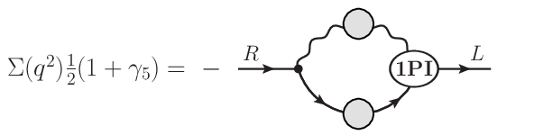
The argument above contains an implicit assumption that sets the scale for decoupling, i.e. that for momenta , the fermions are very “heavy” relative to and so decouple. We show below that QCD is not tenable if that assertion is believed.
Fortunately for QCD, a natural extension of the perturbative Appelquist-Carazzone theorem [98] to include dimensionally transmuted scales such as indicates that it is the current mass which matters. In chiral perturbation theory, both and tend to zero such that is finite, so decoupling does not occur. It is also reassuring that the existence of gluonic condensates does not cause gluons to decouple. More generally, dimensionally transmuted scales 0 are allowed in the extreme IR limit of QCD and (by analogy) TC. These observations hold irrespective of whether an IR fixed point exists or not, so if it exists, nothing prevents it from realizing scale invariance in the NG mode.
Consider QCD at low energies, with the , and quarks decoupled. In the limit of chiral symmetry, low-energy theorems can be derived for amplitudes involving the eight chiral NG bosons and local operators such as chiral currents and . For amplitudes with non-NG states excluded, soft-meson theorems are derivable when all external momenta tend to zero. The key point is that this soft-meson limit and the IR limit of the running of for are indistinguishable: the results of applying chiral perturbation theory and the RG must match. An assumption that decouple in the IR limit would imply decoupling of , and and so contradict the well-known soft-meson theorems for these NG bosons required by chiral perturbation theory. That would be a disaster for QCD.
Instead, what happens is that , and exist in the IR limit of QCD. There are two main possibilities:
- (a)
There is no IR fixed point; rather, runs to with scale invariance explicitly broken. Standard chiral perturbation theory is applicable.
- (b)
It is important to check that these conclusions are consistent with the Appelquist-Carazzone theorem. It states that, to all orders in a perturbative gauge theory, a field with a large Lagrangian mass decouples in the limit taken at fixed renormalization scale , with finite changes in other renormalization constants such as the gauge coupling . Since dimensionally transmuted constants such as those associated with fermion condensation are nonperturbative, as is evident from the discussion of Eq. (31), the proof of Appelquist and Carazzone effectively assumes that all vanish. So at first sight, the theorem is irrelevant, and nothing needs to be checked.
However, it is reasonable to suppose that the Appelquist-Carazzone theorem could be extended to include constants with the conditions of the theorem otherwise unchanged. First, it is necessary to identify RG invariants associated with the field with a large current mass ; either they tend to with , such as particle thresholds for heavy-quark production in QCD, or they vanish because they involve Green’s functions like which depend on that field. Then, for RG invariants that remain in the residual theory after decoupling, there would be a finite change due e.g. to the finite renormalization of and in Eq. (31). This is just a consistency argument, not a derivation, but we suggest that a reasonable derivation may be possible using Landau’s diagrammatic analysis of the nonperturbative behavior of vertex functions [171]. Although this extension of the theorem appears not to have been stated, much less derived, it is implicit in nonperturbative applications such as the decoupling of , and in the presence of light-quark condensates such as .
Following Appelquist and Carazzone [98], let us scale the theorem’s conditions such that the limit for finite momenta is replaced by the IR limit at fixed , with fixed in both cases (mass-independent renormalization). In perturbation theory, that works if all masses are scaled with , so that, in the IR-limit version of the theorem, they tend to zero with .
The problem is that the same argument applied to the -dependent extension of the theorem would require to scale with , and not with the heavy current mass . In the finite- version of the theorem, all remain finite or vanish as ,
| (152) |
so decoupling in the IR limit with fixed can be concluded only if it is assumed that all vanish.
Clearly, decoupling is a consequence of a current mass being large relative to dimensionally transmuted scales in the residual theory. Light-quark condensates and their TC analogues do not decouple in the chiral IR limit.
Appendix B Non-Lagrangian methods for chiral and conformal NG bosons
The NG mode for a symmetry is usually explained in terms of symmetric Lagrangians with potential functions that have flat directions. This obscures the more general understanding developed in the 1960s [172, 173] that currents and their divergences are all that is needed. As preparation for the scaling application in Sec. II, we present a brief review of the analysis for chiral symmetry, and extend it to scale and conformal invariance, where the currents are nonlocal.
The aim is to derive theorems for NG mesons carrying soft momenta as the symmetry limit for current divergences is taken. There are two ways of proceeding (Appendices B.1 and B.2 below); the choice depends on the order in which these limits are taken. This matters because there can be factors involving the pseudo-NG mass for which the limits do not commute, e.g.
| (153) |
but as long as this lack of uniformity is respected, the answer ends up being the same. Scale and conformal invariance are considered in Appendix B.3.
B.1 Chiral-symmetric theory
Consider a chiral -symmetric TC theory with conserved axial-vector currents and axial charges
| (154) |
For any operator (or operator product) which is not chiral invariant, there is another operator
| (155) |
A nonzero VEV of can occur only if is not chiral invariant. Then the amplitude
| (156) |
is called a chiral condensate. In the standard case, is the pseudoscalar operator :
| (157) |
Let be a local spin-0 operator . Then the Ward identity for the time-ordered amplitude
| (158) |
is given by
| (159) |
At zero momentum , Eq. (159) reduces to
| (160) |
which is possible only if has an singularity. This implies Goldstone’s theorem: such a singularity can arise only if there are massless technipions coupled to ,
| (161) |
where the decay constant is defined by
| (162) |
Equation (160) fixes the residue of the pole in Eq. (161). The result is a standard soft- theorem
| (163) |
B.2 Chiral currents partially conserved
The alternative 1960s procedure is to give the currents small divergences
| (164) |
by letting each techniquark have a small renormalized mass and then take the symmetry limit . This is the forerunner of our approach in Sec. II, where the scale-breaking divergence tends to zero as approaches the fixed point .
For massive TC fermions, the Ward identity (159) is replaced by
| (165) |
The traditional derivation of the soft- theorem then runs as follows [173]. The NG bosons acquire mass, so cannot have a singularity, and the limit of Eq. (165) is
| (166) |
where the commutators (155) are now understood to be taken at equal times. The second term is a zero-momentum insertion of the current divergence . It can be nonzero in the limit only if there exists a single-particle intermediate state which becomes massless as
| (167) |
When the residue of this pole is evaluated via , the soft- result (163) is recovered. Note that pole dominance is not assumed: in the symmetry limit, branch cuts are less singular than poles.
B.3 Soft-dilaton theorems for scale and conformal invariance
Goldstone’s theorem, that the number of NG bosons equals the number of independent group generators which transform the vacuum, is generally valid only for local currents. A separate analysis is necessary for nonlocal operators such as the dilatation and conformal currents
| (168) |
which correspond to generators
| (169) |
Given these definitions, the partial conservation equations
| (170) |
show that scale invariance ensures conformal invariance.
The result that only one NG boson is needed—the dilaton of scale invariance—was not obvious at first [101, 102], but it was quickly realized [9] that conformal-invariant Lagrangians can be constructed by having the derivatives of the dilaton field act as Goldstone fields for the four conformal generators . Also, Eq. (170) shows that a pseudo-NG boson for either scale or conformal invariance must have spin 0. The absence of extra NG bosons has been attributed [174, 175, 176] to the failure of to commute with the translation generators in the limit of conformal invariance,
| (171) |
where generate Lorentz transformations.
The literature on the NG mode for scale and conformal invariance is dominated by Lagrangian models of scale invariance. Unlike the chiral case [122, 137, 177], the model independence of their predictions for multiple soft-dilaton emission has yet to be proven explicitly, and they have not been used at all to obtain conformal theorems. Instead, soft-dilaton results for special conformal transformations [52, 53, 54] were obtained by the non-Lagrangian method, which we consider now. It is model independent and resembles the chiral version discussed in Appendices B.1 and B.2, but there are some interesting differences which are best seen for the symmetric case .
We begin with the analogue of Appendix B.1 for scale symmetry ( conserved), excluding for a moment the special case of a single spin-0 operator . Instead of , let us consider a T-ordered product of (not necessarily spin-0) and Fourier transforms
| (172) |
of other local operators , and hence connected momentum-space amplitudes with the function for momentum conservation removed.
The general amplitude involving the dilatation current can be written as
| (173) |
where is constructed entirely from local operators, including the traceless tensor :
| (174) |
Then the scaling Ward identity for takes the form
| (175) |
For scale invariance in the NG mode, the vacuum state is not scale invariant, so there will be operators for which the right-hand side of Eq. (175) does not vanish in the limit of zero momentum :
| (176) |
Equation (176) can be satisfied only if there is a singularity in as :
| (177) |
Since this result includes amplitudes where internal momentum transfers are not light-like, the pole must be due to a massless spin-0 particle, the dilaton . The residue of the pole can be determined from Eq. (1) for the decay constant . Given that has dynamical dimension ,
| (178) |
the pole term in Eq. (177) implies the result
| (179) |
which is a standard soft- theorem.2424 24 The earliest example appeared in Sec. 5 of [50]. The model in Sec. 4 is an almost scale-invariant version of the linear sigma model [178, 74] (clarified in the Appendix of Ref. [179]); it was not used to derive the soft-dilaton theorem.
The case where T is just a single spin-0 operator is special. Consider the unordered amplitude
| (180) |
It has the remarkable property that momentum conservation and scale invariance determine its nonperturbative dependence on :
| (181) |
Time ordering introduces a constant ambiguity2525 25 Notice that cannot be chosen such that is conserved and has zero trace. That will not matter. ,
| (182) |
but the dependence on drops out when is time ordered:
| (183) |
The Ward identity which follows
| (184) |
has a -independent right-hand side, so there is no need to expand about . From2626 26 Spin-0 operators are defined such that an extra term on the right-hand side does not appear. See Appendix C.1.
| (185) |
we see that Eq. (184) fixes the constant in Eq. (181):
| (186) |
When the completeness sum is inserted between and in Eq. (180), only single-dilaton states can reproduce this dependence. So without approximating, we can relate to the dilaton decay constant of Eq. (1):
| (187) |
Comparison of Eqs. (186) and (187) yields the soft-dilaton formula (17).
If scale invariance is in the NG mode, so also is conformal invariance: because of the identity
| (188) |
implied by Eq. (171) and Poincaré invariance of the vacuum. For the conformal current , the analogue of Eq. (173) is
| (189) |
Then gives a conformal Ward identity similar to Eq. (175) but with replaced by in equal-time commutators. In the limit , the result is
| (190) |
which is nonzero only if there is a singular term in :
| (191) |
Therefore, Eqs. (176) and (177) can be extended to include the pole term:2727 27 The connection between terms and special conformal transformations was noted in Ref. [180] and used to derive soft-dilaton theorems [52] long ago. The subject has been revived very recently [53, 54]; note the important distinction they made between NG-mode dilatons and “gravitational dilatons”.
| (192) |
Although appears as a projection in a light-like direction (), all space-like directions and hence individual components can be obtained by comparing states with small on-shell momenta and . The general soft- result for special conformal transformations is therefore
| (193) |
As is well known [51, 179, 181], the commutators are best classified via the little group at . Each time commutes with a dimension- operator, it reduces the dimension to . So there are towers of local operators (mostly derivatives of other operators) above familiar spin- operators of minimal dimension such as chiral currents and whose commutators necessarily vanish at . For all operators of this type, we have
| (194) |
where generate the Lorentz group and are the corresponding spin matrices for . Translating with yields the standard formula
| (195) |
So for operators , Eq. (193) implies
| (196) |
The soft-dilaton theorems (179) and (196) will be needed in Appendix D.
Appendix C Nonperturbative definition of gluon and technigluon condensates
Definitions of the gluon condensate and its TC analogue are problematic because
- (1)
they are perturbatively divergent nonperturbative quantities, and
- (2)
they involve operators like which are hard to separate from the identity operator under renormalization or within operator product expansions.
The issue arises in the discussion following Eq. (7), where the spectator operator is used to obtain soft-dilaton results such as Eq. (15) and hence Eq. (53) for the technigluon condensate. To avoid ambiguity, we require that be multiplicatively renormalizable2828 28 In QCD with , mixing with must also be considered [100, 182]. and (in the sense of that discussion) independent.
In this appendix, we explain the need for these requirements, noting that, while they serve our purposes and are consistent with various proposals to define , the results still lack sufficient precision for unambiguous calculations, e.g. on the lattice. The extent to which a definitive nonperturbative definition is possible is then considered. The analysis refers to the physical region, which is if there is an IR fixed point , and if not ().
When the gauge coupling is finite, functional integrals for Green’s functions are dominated by nonperturbative gauge [183] and fermion fields. Evidently these fields are hard to characterize analytically, i.e. beyond numerical lattice methods. Instead, attention is focused on a few physical operators that form nonperturbative condensates which can be given theoretical and phenomenological meaning. The problem is to define without introducing ambiguities proportional to the identity operator . Only then does the condensate acquire a physical meaning.
Even before QCD was invented, it was known how to do this for divergences of partially conserved currents [99]: they belong to an irreducible representation of an equal-time non-Abelian chiral group which distinguishes them from the chiral-invariant operator . For example, if and appear in an operator product expansion, their contributions to its VEV can be distinguished, provided that other operators with poorly defined condensates are known to have less singular coefficient functions.
In gauge theories, these chiral condensates are formed when is a fermion bilinear: for QCD and for TC. As long as the renormalization procedure respects chiral symmetry, these operators do not have counterterms proportional to and so belong to an irreducible chiral representation. The corresponding condensates are necessarily nonperturbative, so they produce power corrections to short-distance expansions of operator products.
However, any discussion of power corrections at short distances in QCD would be incomplete without including terms induced by the gluon condensate [69, 64] formed when is the operator . Then group theory cannot be used to distinguish from , so the definition of remains ambiguous due to counterterms proportional to . The same problem arises for the technigluon condensate .
A practical approach still in use [184, 185, 186] is to impose a regulator such as the lattice and then identify and subtract perturbative contributions to up to some high but finite order. The series is not expected to converge because of renormalons, but perturbative coefficients can be checked numerically to see if their behavior is consistent with Borel summability. The theoretical argument for this is that, if all orders of perturbation theory can in principle be summed by a well-defined technique and the result is then subtracted, the remainder will be the nonperturbative amplitude being sought [187]. However, even if Borel summability can be proven to all orders, Borel’s method is not unique: nonperturbative dynamics may choose another well-defined procedure. Generally, there is no guarantee that nonperturbative amplitudes can be deduced from purely perturbative considerations [188, 189], so it is not surprising that these issues remain a source of unease [3].
Another idea is to multiply by and use RG invariance. Since purely nonperturbative constants can have no Taylor series about (as noted for the constant in Eq. (31)), perturbative terms cannot be invariant. But that is not sufficient, because nothing has been done to distinguish the desired operator from . For example, if and appear in the expansion of a product of physical currents, can mix with the VEV of the term under RG transformations.
Our proposal is to consider the scaling properties of operators, not just amplitudes. We consider mainly the TC case where chiral symmetry of the Lagrangian stops from mixing with techniquark bilinears.
Let set the scale for an arbitrary renormalization prescription for composite operators , including the trace operator
| (197) |
We need to distinguish the results of variations at fixed coupling and the total variation
| (198) |
Because subtractions necessarily include perturbative terms, we do not expect the result to be exactly RG invariant — there must be mixing with ,
| (199) |
where is an ordinary function. However, the -dependent term can be absorbed into the definition of the trace operator
| (200) |
where is a constant independent of and . Note that the integral over takes account of the dependence of . Evidently the resulting operator is RG invariant:
| (201) |
We are not done, because the solution of Eq. (201) is not unique. Any ordinary function whose dependence on and is carried solely by the RG invariant mass of Eq. (31) is itself RG invariant. Therefore all operators
| (202) |
are RG invariant. To preserve engineering dimensions, can be chosen to be times a constant independent of and . This ambiguity does not affect the multiplicative renormalizability of operators obtained by multiplying by -dependent factors.
Nevertheless, it is necessary to eliminate the ambiguity (202) if soft-dilaton results such as Eq. (15) are to be derivable. That happens when we apply the -independence criterion to
| (203) |
for use as a spectator operator in the insertion rule (9), because
| (204) |
implies
| (205) |
Then has no ambiguity — in principle.
In practice, we would like to be able to test our soft-dilaton results by comparison with experimental or lattice data. For that, our minimal requirements on are necessary but not sufficient. It is not even clear how to implement them for prescriptions currently on offer for .
Phenomenology is based on the original QCD prescription [64, 69, 190], where -independent power corrections in the small- expansion of two electromagnetic currents
| (206) |
are by definition contained entirely within the gluonic coefficient function . Dispersive sum rules for the operator product (206) are reasonably consistent with each other for , but there is no reason to suppose that a similar definition of the gluon condensate for a different operator product would be equivalent.
The idea of this definition is to suppose that the term in a short-distance expansion is purely perturbative. That is a difficult concept: even if is truncated to a polynomial in , the running of depends on dimensionally transmuted masses which can produce power corrections.2929 29 Sometimes the presence of nonperturbative power corrections is attributed to a “breakdown” of the Wilson expansion. It is true that a fully rigorous proof [191] has so far been possible only within perturbation theory, but Wilson and Zimmermann [192] gave convincing arguments for operator product expansions to be valid in any nonperturbative theory consistent with axiomatic field theory. See also Ref. [193]. And it is unclear how this proposal can be related to purely theoretical definitions, where perturbative truncation is also a problem. Examples are directly estimating the one-point function on the lattice (noted above), or adding a heavy fermion and taking its mass to :
| (207) |
A way around this impasse may be to use experimental data to extend beyond the UV region where asymptotic freedom is applicable. If can be measured at finite values where the small- expansion is no longer valid, perturbative truncation would not be needed. This would have to be done within a renormalization scheme suitable for matching to lattice calculations at these intermediate non-UV energies. Then, if the thermodynamic limit can be demonstrated for the Euclidean partition function on the lattice,
| (208) |
a practical nonperturbative definition of the Euclidean condensate would be
| (209) |
Eq. (209) is equivalent to a condition [75, 194] arising from the Feynman-Hellmann theorem.
In crawling TC, where there is a fixed point , the technigluon condensate at appears in results such as Eqs. 50) and (53). It is obtained as a limit of the amplitude
| (210) |
where . The operator is local, so the amplitude (210) is a one-point function where intermediate states such as cannot occur. It follows that is continuous in the scaling limit:
| (211) |
C.1 Relation to commutators with the dilatation generator
A conventional soft-dilaton theorem such as Eq. (17) is valid for operators which scale homogeneously with operator dimension , i.e.
| (212) |
with other operators absent. As seen above, if has spin , mixing with the identity operator is hard to control, producing ambiguities such as Eq. (202). Since Eq. (212) is not invariant under the shift ( = const.),
| (213) |
it could act as an alternative to independence as a criterion for resolving the ambiguity in Eq. (203). These commutators (equal-time for where is not conserved) are determined by short-distance expansions of . As noted in Sec. II [footnote 5 and Eq. (27)], short-distance behavior for is determined by the fixed point (asymptotic freedom), whereas, when is first fixed at , it cannot run: short-distance behavior is then controlled by the nonperturbative world at (Appendix D). Therefore the cases and must be considered separately.
At , the condition (212) would resolve the ambiguity in spin- operators , e.g. the operator in the mass formula (53) with identified as [Eqs. (51) and (249)]. However, we have been unable to relate this to the -independence criterion for the operator (203) which defines in the mass formula. In Eq. (9), we considered replacing by in order to obtain a scaling Ward identity, but could not circumvent the facts that Eq. (9) is valid only for and the limits and do not commute. In Appendices B and D, we assume that spin- operators can be classified according to the condition (212).
In all cases , the relevant operator product expansion for spin- operators takes the form
| (214) |
where the constant has mass dimension 4, and where the leading singularities
| (215) | ||||
| (216) |
have dependence determined by conservation and tracelessness in the indices ; [compare Eq. (181)]. Here the prescription for unordered products should be understood, so we have with no term25 and can define to be . The coefficient function is normalized to produce the correct commutators of with the Poincaré generators and . It also corresponds to the term in Eq. (212).
At where , is both traceless and conserved and hence proportional to . Therefore, given the presence of the term in Eq. (214), we can set . The commutator condition (212) is reproduced if we set
| (217) |
On the lattice, it would be hard to insulate a test of this condition from effects.
For , the problem is that asymptotic freedom and the trace anomaly require the coefficient function
| (218) |
to be far more singular than the coefficient function .
For example, let be the RG-invariant trace operator discussed in Eqs. (197) and (202). Then asymptotic freedom requires the trace amplitude
| (219) |
to have the following short-distance behavior,
| (220) |
where is a constant and is the one-loop -function coefficient (23). That corresponds to
| (221) |
and hence
| (222) |
which is compared with Eq. (215) for as .
Since is RG invariant, it can be written as a function of and a dimensionally transmuted scale :
| (223) |
It is therefore likely that an expansion of contains a nonleading term whose contribution to in Eq. (214) cannot be distinguished from . Then the latter term should be absorbed into by setting . We conclude that a study of behavior for does not produce a criterion to resolve the ambiguity (202). All we can say is that asymptotic freedom requires , as noted in Eq. (20), and hence
| (224) |
in the equal-time limit .
Appendix D NG-mode conformal-invariant world at
Unlike a scale-invariant theory in the WW mode, the world at is somewhat similar to the physical world (TC or QCD) for . It has a particle spectrum with
- (1)
non-NG masses close to their physical values, because in the physical world, scale invariance is approximate at low energies, and
- (2)
an NG sector which is massless because at , scale and chiral invariance are exact.
This situation is allowed because amplitudes at can have a complicated dependence on scales set by the dilaton decay constant ( or ) and other dimensionally transmuted masses and condensates. As we emphasize in various sections of this paper, the effects of dependence must be carefully distinguished from those due to an explicit breaking of scale invariance in the Lagrangian, e.g. by fermion mass parameters or Coleman-Weinberg potentials.
In case this picture seems counterintuitive, recall the fact that the NG scaling mode for the ground state at requires it to have a noncompact scaling degeneracy in addition to compact chiral degeneracies. Under a finite scaling transformation, the ground state of a scale-invariant world is transformed to the ground state of another scale-invariant world :
| (225) |
The same is true for all members of a complete set of states for ,
| (226) |
where span the state space of . The well-known identity [179, 10]
| (227) |
implies that if has mass , the mass of is
| (228) |
Clearly this applies generally: all dimensionally transmuted masses associated with a given world are scaled up or down to in the transformed world .
Identities such as Eq. (228) are often quoted as a reason for supposing that a scale- or conformal-invariant world must be entirely unphysical. How can there be a particle spectrum if for every massive particle, there is a continuum of particles [195] with the same quantum numbers except for their mass, which ranges from infinitesimal values to infinity? Must we conclude that we have an unparticle theory [128] with power-law branch cuts at zero-momentum thresholds, or that particles, if they exist, are necessarily massless, as in free-field theory?
To answer these concerns, note that such arguments depend on an implicit assumption that the ground state is either unique or that, while it may exhibit a compact chiral degeneracy, it lacks the scaling degeneracy specified by Eq. (225). Scaling degeneracy changes the picture completely, because different members of each particle continuum belong to different worlds.
Consider observers and in their respective universes, and . Assume that these observers choose (say) natural units when making measurements. Since these units involve reference to a dimensionally transmuted mass, a scale transformation necessarily scales the units used in to those in , e.g.
| (229) |
Since no observer is able to compare measurements in different worlds, all experimental data in one world would be exactly the same as in another world. Therefore these worlds must be physically equivalent, as is the case for any other symmetry with a vacuum degeneracy. Each observer could rely on the same scale-invariant version of the PDG tables, i.e. with particle masses at differing slightly from those of our world , as described above.
Crawling TC picks out one of these scale-degenerate vacua via tiny values of the parameter which cause scale invariance to be broken explicitly by the nonvanishing trace anomaly on .
Clearly, conformal group theory fails for -dependent amplitudes at . However, it has always been accepted that symmetries of the Hamiltonian, whether hidden or approximate, become exact for coefficient functions in short-distance expansions. These rules were originally proposed [66] for approximate scale and chiral symmetry (hidden in the chiral case), and later applied to hidden scale and conformal invariance [196]. Subsequently, asymptotic chiral invariance was derived from soft-pion identities [65]. Here we extend this method to derive asymptotic scale and conformal invariance from the soft-dilaton theorems (179) and (196).
We begin with the coordinate-space version of the scaling identity (179) for a general operator product:
| (230) |
In what follows, neighborhoods of coinciding points are excised to avoid time-ordering ambiguities involving and its derivatives, as in Ref. [66]. For a subset of the operators in Eq. (230), there is an operator-product expansion
| (231) |
for the short-distance limit with other coordinates held fixed at values . When Eq. (231) is inserted into each side of Eq. (230), the result is an equivalence between asymptotic expansions:
| (232) |
The soft- amplitude on the left-hand side can be eliminated via Eq. (230)
| (233) |
with the result
| (234) |
Since can be chosen at will, this asymptotic expansion is valid only if all coefficients of vanish:
| (235) |
Therefore all coefficient functions scale with dimension :
| (236) |
This is the same as Wilson’s rule [66] for leading singularities in a theory of WW-mode scale invariance explicitly broken by generalized mass terms such as current fermion masses. The difference is that our result is for all coefficient functions in a theory of exact scale invariance in the NG mode. All dependence on dimensionally transmuted “constituent” masses arises from scale condensates formed from vacuum amplitudes .
The same procedure works for special conformal transformations. We give details for operators of the type (194) which commute with at :
| (237) |
Let the action of an infinitesimal Lorentz transformation on the tensor or spinor indices of an operator inside a field product be denoted as follows:
| (238) |
In coordinate space, the conformal soft- theorem (196) becomes
| (239) |
When the expansion (237) is applied to both sides of Eq. (239), the result for the coefficient function of is
| (240) |
Here we made use of the observation above Eq. (193) that the four components of can be chosen independently. Together with Eq. (236) and Poincaré symmetry, this shows that exact conformal invariance can be applied to asymptotic coefficient functions despite the dependence of amplitudes outside the short-distance region.
Appendix E Scaling dimension of the technigluon (field-strength operator)2
This appendix concerns the origins and derivation of formulas for the anomalous scaling function (51) and dimension of the trace anomaly. These formulas, derived in Refs. [13, 14], were common private knowledge as far back as the 1970s. Only recently, we rediscovered the original version
| (241) |
below Eq. (28) of Ref. [58], where and are given by
| (242) |
For Eq. (51), see also Refs. [61] and [100, 197] (drawn to our attention by R. Zwicky and E. Pallante, respectively).
First, let us review the derivation in Refs. [13, 14] of Eq. (51), simplified for the case of TC with massless fermions. Construct CS equations for RG invariant amplitudes
| (243) |
and apply the operator :
| (244) |
Since is proportional to the amplitude where is inserted at zero momentum into , Eq. (244) implies
| (245) |
where
| (246) |
is the anomalous scaling function (51) in the form given in Refs. [13, 14] and confirmed in Eq. [198]. [There is an incorrect factor of 2 in Eq. (13) of [197].] This result was given originally for massless QCD in the form [100]
| (247) |
which corresponds to Eq. (246) because of the fixed- identity
| (248) |
The dynamical dimension of the technigluon operator in the IR limit is therefore
| (249) |
The same rule holds for a UV fixed point or , which was the context of the original version (241); the relation is a consequence of Eq. (248). In the UV case, the plus sign in is crucial [58] because is negative: scaling corrections have dimension and so do not upset the leading short-distance behavior of operator product expansions.
For an IR fixed point, where , such as in chiral-scale perturbation theory or crawling TC, the expansion is at low energies, so the dimension of scale-breaking terms can be either due to the trace anomaly or (if there are fermion mass terms) . The main proviso is to ensure the condition (mass) for all particles appearing in the expansion.
References
- [1] T. Appelquist and Y. Bai, Light dilaton in walking gauge theories, Phys. Rev. D 82, 071701 (2010). [arXiv:1006.4375]
- [2] M. Hashimoto and K. Yamawaki, Technidilaton at conformal edge, Phys. Rev. D 83, 015008 (2011). [arXiv:1009.5482]
- [3] T. Appelquist et al., Lattice gauge theories at the energy frontier, Proceedings of the 2013 Community Summer Study Planning the future of U.S. particle physics, Division of Particles and Fields (American Physical Society, Minneapolis MN, 2013), arXiv:1309.1206.
- [4] S. Matsuzaki and K. Yamawaki, Dilaton chiral perturbation theory: determining the mass and decay constant of the technidilaton on the lattice, Phys. Rev. Lett. 113, 082002 (2014). [arXiv:1311.3784]
- [5] M. Golterman and Y. Shamir, Low-energy effective action for pions and a dilatonic meson, Phys. Rev. D 94, 054502 (2016). [arXiv:1603.04575]
- [6] C. G. Callan Jr., S. Coleman and R. Jackiw, A new improved energy-momentum tensor, Ann. Phys. (N.Y.) 59, 42 (1970).
- [7] M. Gell-Mann, Symmetry violation in hadron physics, 1969 Hawaii Topical Conference on Particle Physics (Western Periodicals Co., Los Angeles, CA, 1970), p. 168.
- [8] P. G. O. Freund and Y. Nambu, Scalar fields coupled to the trace of the energy-momentum tensor, Phys. Rev. 174, 1741 (1968).
- [9] C. J. Isham, A. Salam and J. A. Strathdee, Broken chiral and conformal symmetry in an effective-Lagrangian formalism, Phys. Rev. D 2, 685 (1970).
- [10] J. R. Ellis, Aspects of conformal symmetry and chirality, Nucl. Phys. B 22, 478 (1970).
- [11] B. Zumino, Effective Lagrangians and broken symmetries, in Lectures on elementary particles and quantum field theory, 1970 Brandeis University Summer Institute in Theoretical Physics, Vol. 2 (M.I.T. Press, Cambridge, MA, 1970), pp. 437-500.
- [12] J. Ellis, Approximate scale and chiral invariance, 1971 Coral Gables Conference Fundamental interactions at high energy, Vol. 2, Broken scale invariance and the light cone, M. Gell-Mann and K. Wilson (Gordon and Breach, New York 1971), p. 77.
- [13] R. J. Crewther and L. C. Tunstall, Origin of rule for kaon decays: QCD infrared fixed point, arXiv:1203.1321.
- [14] R. J. Crewther and L. C. Tunstall, rule for kaon decays derived from QCD infrared fixed point, Phys. Rev. D 91, 034016 (2015). [arXiv:1312.3319]
- [15] R. J. Crewther and L. C. Tunstall, Status of chiral-scale perturbation theory, Proc. Sci. CD15 (2015) 132 [arXiv:1510.01322].
- [16] T. Appelquist, J. Terning and L. C. R. Wijewardhana, Postmodern technicolor, Phys. Rev. Lett. 79, 2767 (1997). [arXiv:hep-ph/9706238]
- [17] K. G. Wilson, The renormalization group and strong interactions, Phys. Rev. D 3, 1818 (1971).
- [18] K. G. Wilson and J. Kogut, The renormalization group and the expansion, Phys. Rep. 12, 75 (1974), Sec. 12.
- [19] E. Marchais, P. Mati, and D. F. Litim, Fixed points and the spontaneous breaking of scale invariance, Phys. Rev. D 95, 125006 (2017). [arXiv:1702.05749]
- [20] T. Appelquist, G. T. Fleming and E. T. Neil, Lattice study of the conformal window in QCD-like theories, Phys. Rev. Lett. 100, 171607 (2008); Erratum, Phys. Rev. Lett. 102, 149902(E) (2009). [arXiv:0712.0609]
- [21] T. Appelquist, G. T. Fleming and E. T. Neil, Lattice study of conformal behavior in Yang-Mills theories, Phys. Rev. D 79, 076010 (2009). [arXiv:0901.3766]
- [22] L. Del Debbio, The conformal window on the lattice, Proc. Sci. LATTICE2010 (2010) 004 [arXiv:1102.4066].
- [23] L. Del Debbio, IR fixed points in lattice field theories, Int. J. Mod. Phys. A 29, 1445006 (2014).
- [24] T. DeGrand, Lattice tests of beyond Standard Model dynamics, Rev. Mod. Phys. 88, 015001 (2016). [arXiv:1510.05018]
- [25] C.-J. D. Lin, K. Ogawa and A. Ramos, The Yang-Mills gradient flow and gauge theory with 12 massless fundamental fermions in a colour-twisted box, JHEP 1512, 103 (2015). [arXiv:1510.05755]
- [26] Z. Fodor, K. Holland, J. Kuti, S. Mondal, D. Nogradi and C. H. Wong, Fate of the conformal fixed point with twelve massless fermions and gauge group, Phys. Rev. D 94, 091501 (2016). [arXiv:1607.06121]
- [27] A. Hasenfratz and D. Schaich, Nonperturbative beta function of twelve-flavor gauge theory, JHEP 1802, 132 (2018). [arXiv:1610.10004]
- [28] A. Deur, S. J. Brodsky and G. F. de Téramond, The QCD running coupling, Prog. Part. Nucl. Phys. 90, 1 (2016). [arXiv:1604.08082]
- [29] R. J. Crewther, Broken scale invariance and the width of a single dilaton, Phys. Lett. B 33, 305 (1970).
- [30] E. Gildener and S. Weinberg, Symmetry breaking and scalar bosons, Phys. Rev. D 13, 3333 (1976).
- [31] S. Fubini, A new approach to conformal invariant field theories, Nuovo Cimento A 34, 521 (1976).
- [32] T. Appelquist and C. W. Bernard, Strongly interacting Higgs bosons, Phys. Rev. D 22, 200 (1980).
- [33] A. C. Longhitano, Heavy Higgs bosons in the Weinberg-Salam model, Phys. Rev. D 22, 1166 (1980).
- [34] G. Buchalla and O. Catà, Effective theory of a dynamically broken electroweak Standard Model at NLO, JHEP 1207, 101 (2012). [arXiv:1203.6510]
- [35] F. Feruglio, The chiral approach to the electroweak interactions, Int. J. Mod. Phys. A 8, 4937 (1993). [arXiv:hep-ph/9301281]
- [36] J. Bagger, V. D. Barger, K. Cheung, J. F. Gunion, T. Han, G. A. Ladinsky, R. Rosenfeld and C.-P. Yuan, The strongly interacting system: gold-plated modes, Phys. Rev. D 49, 1246 (1994). [arXiv:hep-ph/9306256]
- [37] V. Koulovassilopoulos and R. S. Chivukula, The phenomenology of a nonstandard Higgs boson in scattering, Phys. Rev. D 50, 3218 (1994). [arXiv:hep-ph/9312317]
- [38] C. P. Burgess, J. Matias and M. Pospelov, A Higgs or not a Higgs? What to do if you discover a new scalar particle, Int. J. Mod. Phys. A 17, 1841 (2002). [arXiv:hep-ph/9912459]
- [39] S.-Z. Wang and Q. Wang, Electroweak chiral Lagrangian for neutral Higgs boson, Chin. Phys. Lett. 25, 1984 (2008).
- [40] B. Grinstein and M. Trott, A Higgs-Higgs bound state due to new physics at a TeV, Phys. Rev. D 76, 073002 (2007). [arXiv:0704.1505]
- [41] R. Contino, C. Grojean, M. Moretti, F. Piccinini and R. Rattazzi, Strong double Higgs production at the LHC, JHEP 1005, 89 (2010). [arXiv:1002.1011]
- [42] R. Alonso, M. B. Gavela, L. Merlo, S. Rigolin and J. Yepes, The effective chiral Lagrangian for a light dynamical “Higgs particle”, Phys. Lett. B 722, 330 (2013) [Erratum ibid 726, 926 (2013)]. [arXiv:1212.3305]
- [43] G. Buchalla, O. Catà and C. Krause, Complete electroweak chiral Lagrangian with a light Higgs at NLO, Nucl. Phys. B 880, 552 (2014). [arXiv:1307.5017]
- [44] T. Appelquist, J. Ingoldby and M. Piai, Dilaton EFT framework for lattice data, JHEP 1707, 035 (2017). [arXiv:1702.04410]
- [45] T. Appelquist, J. Ingoldby and M. Piai, Analysis of a dilaton EFT for lattice data, JHEP 1803, 039 (2018). [arXiv:1711.00067]
- [46] Y. Aoki et al. [LatKMI Collaboration], Light composite scalar in eight-flavor QCD on the lattice, Phys. Rev. D 89, 111502(R) (2014). [arXiv:1403.5000]
- [47] Y. Aoki et al. [LatKMI Collaboration], Light flavor-singlet scalars and walking signals in QCD on the lattice, Phys. Rev. D 96, 014508 (2017). [arXiv:1610.07011]
- [48] T. Appelquist et al. [LSD Collaboration], Strongly interacting dynamics and search for new physics at the LHC, Phys. Rev. D 93, 114514 (2016). [arXiv:1601.04027]
- [49] T. Appelquist et al. [LSD Collaboration], Nonperturbative investigations of gauge theory with eight dynamical flavors, Phys. Rev. D 99, 014509 (2019). [arXiv:1807.08411]
- [50] G. Mack, Partially conserved dilatation current, Nucl. Phys. B 5, 499 (1968).
- [51] P. Carruthers, Broken scale invariance in particle physics, Phys. Rept. 1, 1 (1971).
- [52] R. J. Crewther, Spontaneous breakdown of conformal and chiral invariance, Phys. Rev. D 3, 3152 (1971); [Erratum 4, 3814(E) (1971)].
- [53] P. Di Vecchia, R. Marotta, M. Mojaza, and J. Nohle, New soft theorems for the gravity dilaton and the Nambu-Goldstone dilaton at subsubleading order, Phys. Rev. D 93, 085015 (2016). [arXiv:1512.03316]
- [54] P. Di Vecchia, R. Marotta, and M. Mojaza, Double-soft behavior of the dilaton of spontaneously broken conformal invariance, JHEP 09, 001 (2017). [arXiv:1705.06175]
- [55] R. F. Dashen, Chiral as a symmetry of the strong interactions, Phys. Rev. 183, 1245 (1969), end of section IIC.
- [56] P. Minkowski, On the anomalous divergence of the dilatation current in gauge theories, Berne PRINT-76-0813, 1976.
- [57] S. L. Adler, J. C. Collins and A. Duncan, Energy-momentum-tensor trace anomaly in spin 1/2 quantum electrodynamics, Phys. Rev. D 15, 1712 (1977).
- [58] N. K. Nielsen, The energy momentum tensor in a non-Abelian quark gluon theory, Nucl. Phys. B120, 212 (1977).
- [59] J. C. Collins, A. Duncan and S. D. Joglekar, Trace and dilatation anomalies in gauge theories, Phys. Rev. D 16, 438 (1977).
- [60] P. Breitenlohner and D. Maison, Dimensional renormalization and the action principle, Comm. Math. Phys. 52, 11 (1977).
- [61] V. P. Spiridonov, Anomalous dimension of and -function, Institute for Nuclear Research (Moscow) IYal-P-0378 (1984).
- [62] V. A. Novikov, M. A. Shifman, A. I. Vainshtein and V. I. Zakharov, Are all hadrons alike?, Nucl. Phys. B 191, 301 (1981).
- [63] J. C. Collins, Renormalization, Cambridge University Press, (Cambridge 1984), section 6.7.
- [64] A. I. Vainshtein, V. I. Zakharov and M. A. Shifman, Gluon condensate and leptonic decays of vector mesons, Pis’ma Eksp. Teor. Fiz. 27, 60 (1978); trans. JETP Lett. 27, 55 (1978).
- [65] C. Bernard, A. Duncan, J. LoSecco, and S. Weinberg, Exact spectral-function sum rules, Phys. Rev. D 12, 792 (1975), appendix.
- [66] K. G. Wilson, Non-Lagrangian models of current algebra, Phys. Rev. 179, 1499 (1969).
- [67] S. Coleman and E. Weinberg, Radiative corrections as the origin of spontaneous symmetry breaking, Phys. Rev. D 7, 1888 (1973).
- [68] M. Bando, K. Matumoto and K. Yamawaki, Technidilaton, Phys. Lett. B 178, 308 (1986).
- [69] M. A. Shifman, A. I. Vainshtein and V. I. Zakharov, QCD and resonance physics. Theoretical foundations, Nucl. Phys. B 147, 385 (1979).
- [70] L. Del Debbio and R. Zwicky, Hyperscaling relations in mass-deformed conformal gauge theories, Phys. Rev. D 82, 014502 (2010). [arXiv:1005.2371]
- [71] L. Del Debbio and R. Zwicky, Scaling relations for the entire spectrum in mass-deformed conformal gauge theories, Phys. Lett. B 700, 217 (2011). [arXiv:1009.2894]
- [72] L. Del Debbio and R. Zwicky, Conformal scaling and the size of -hadrons, Phys. Rev. D 89, 014503 (2014). [arXiv:1306.4038].
- [73] T. Appelquist et al. [LSD Collaboration], Toward TeV conformality, Phys. Rev. Lett. 104, 071601 (2010). [arXiv:0910.2224]
- [74] M. Gell-Mann, Symmetries of baryons and mesons, Phys. Rev. 125, 1067 (1962), footnote 38.
- [75] L. Del Debbio and R. Zwicky, Renormalisation group, trace anomaly and Feynman-Hellmann theorem, Phys. Lett. B 734, 107 (2014). [arXiv:1306.4274]
- [76] S. Weinberg, Implications of dynamical symmetry breaking, Phys. Rev. D 13, 974 (1976).
- [77] S. Weinberg, Implications of dynamical symmetry breaking: an addendum, Phys. Rev. D 19, 1277 (1979).
- [78] L. Susskind, Dynamics of spontaneous symmetry breaking in the Weinberg-Salam theory, Phys. Rev. D 20, 2619 (1979).
- [79] I. Caprini, G. Colangelo, and H. Leutwyler, Mass and width of the lowest resonance in QCD, Phys. Rev. Lett. 96, 132001 (2006). [arXiv:hep-ph/0512364]
- [80] M. Tanabashi et al. (Particle Data Group), Review of particle physics, Phys. Rev. D 98, 030001 (2018).
- [81] J. R. Pelaéz, From controversy to precision on the sigma meson: a review on the status of the non-ordinary resonance, Phys. Rept. 658, 1 (2016). [arXiv:1510.00653]
- [82] G. Aad et al. [ATLAS Collaboration], Observation of a new particle in the search for the Standard Model Higgs boson with the ATLAS detector at the LHC, Phys. Lett. B 716, 1 (2012). [arXiv:1207.7214]
- [83] S. Chatrchyan et al. [CMS Collaboration], Observation of a new boson at a mass of 125 GeV with the CMS experiment at the LHC, Phys. Lett. B 716, 30 (2012). [arXiv:1207.7235]
- [84] F. Sannino, Conformal dynamics for TeV physics and cosmology, Acta Phys. Polon. B 40, 3533 (2009), subsections E.2 and E.3.3. [arXiv:0911.0931]
- [85] S. Weinberg, Approximate symmetries and pseudo-Goldstone bosons, Phys. Rev. Lett. 29, 1698 (1972).
- [86] H. Georgi and A. Pais, Vacuum symmetry and the pseudo-Goldstone phenomenon, Phys. Rev. D 12, 508 (1975).
- [87] D. B. Kaplan and H. Georgi, breaking by vacuum misalignment, Phys. Lett. B 136, 183 (1984).
- [88] D. B. Kaplan, H. Georgi and S. Dimopoulos, Composite Higgs scalars, Phys. Lett. B 136, 187 (1984).
- [89] H. Georgi, D. B. Kaplan and P. Galison, Calculation of the composite Higgs mass, Phys. Lett. B 143, 152 (1984).
- [90] H. Georgi and D. B. Kaplan, Composite Higgs and custodial , Phys. Lett. B 145, 216 (1984).
- [91] M. J. Dugan, H. Georgi and D. B. Kaplan, Anatomy of a composite Higgs model, Nucl. Phys. B 254, 299 (1985).
- [92] K. Agashe, R. Contino and A. Pomarol, The minimal composite Higgs model, Nucl. Phys. B 719, 165 (2005). [arXiv:hep-ph/0412089]
- [93] R. Contino, L. Da Rold and A. Pomarol, Light custodians in natural composite Higgs models, Phys. Rev. D 75, 055014 (2007). [arXiv:hep-ph/0612048]
- [94] G. F. Giudice, C. Grojean, A. Pomarol and R. Rattazzi, The strongly-interacting light Higgs, JHEP 0706, 45 (2007). [arXiv:hep-ph/0703164]
- [95] C. Csáki, C. Grojean and J. Terning, Alternatives to an elementary Higgs, Rev. Mod. Phys. 88, 045001 (2016). [arXiv:1512.00468]
- [96] J. R. Ellis, M. K. Gaillard and D. V. Nanopoulos, A phenomenological profile of the Higgs boson, Nucl. Phys. B 106, 292 (1976).
- [97] D. D. Dietrich, F. Sannino and K. Tuominen, Light composite Higgs from higher representations versus electroweak precision measurements: Predictions for CERN LHC, Phys. Rev. D 72, 055001 (2005). [arXiv:hep-ph/0505059]
- [98] T. Appelquist and J. Carazzone, Infrared singularities and massive fields, Phys. Rev. D 11, 2856 (1975).
- [99] M. Gell-Mann, R. J. Oakes and B. Renner, Behavior of current divergences under , Phys. Rev. 175, 2195 (1968).
- [100] B. Grinstein and L. Randall, The renormalization of , Phys. Lett. B 217, 335 (1989).
- [101] A. Salam and J. A. Strathdee, Nonlinear realizations. 2. Conformal symmetry, Phys. Rev. 184, 1760 (1969).
- [102] C. J. Isham, A. Salam and J. A. Strathdee, Spontaneous breakdown of conformal symmetry, Phys. Lett. B 31, 300 (1970).
- [103] K. A. Meissner and H. Nicolai, Conformal symmetry and the standard model, Phys. Lett. B 648, 312 (2007). [arXiv:hep-th/0612165]
- [104] W. F. Chang, J. N. Ng and J. M. S. Wu, Shadow Higgs boson from a scale-invariant hidden model, Phys. Rev. D 75, 115016 (2007). [arXiv:hep-ph/0701254]
- [105] R. Foot, A. Kobakhidze and R. R. Volkas, Electroweak Higgs as a pseudo-Goldstone boson of broken scale invariance, Phys. Lett. B 655, 156 (2007). [arXiv:0704.1165]
- [106] W. D. Goldberger, B. Grinstein and W. Skiba, Distinguishing the Higgs boson from the dilaton at the Large Hadron Collider, Phys. Rev. Lett. 100, 111802 (2008). [arXiv:0708.1463]
- [107] L. Vecchi, Phenomenology of a light scalar: the dilaton, Phys. Rev. D 82, 076009 (2010). [arXiv:1002.1721]
- [108] B. Bellazzini, C. Csáki, J. Hubisz, J. Serra and J. Terning, A Higgs-like dilaton, Eur. Phys. J. C 73, 2333 (2013). [arXiv:1209.3299]
- [109] B. Bellazzini, C. Csáki, J. Hubisz, J. Serra and J. Terning, A naturally light dilaton and a small cosmological constant, Eur. Phys. J. C 74, 2790 (2014). [arXiv:1305.3919]
- [110] F. Coradeschi, P. Lodone, D. Pappadopulo, R. Rattazzi and L. Vitale, A naturally light dilaton, JHEP 1311, 057 (2013). [arXiv:1306.4601]
- [111] Y.-M. P. Lam, Nonlinear chiral symmetry and partial conservation of axial-vector current—Bogoliubov-Parasiuk-Hepp-Zimmermann renormalization, Phys. Rev. D 7, 2950 (1973).
- [112] J. Gasser and H. Leutwyler, Chiral perturbation theory to one loop, Annals Phys. 158, 142 (1984).
- [113] J. Gasser and H. Leutwyler, Chiral perturbation theory: expansions in the mass of the strange quark, Nucl. Phys. B 250, 465 (1985).
- [114] H. Georgi, Weak interactions and modern particle theory (Benjamin/Cummings, Menlo Park, 1984).
- [115] J. Gasser, M. E. Sainio and A. varc, Nucleons with chiral loops, Nucl. Phys. B307, 779 (1988).
- [116] S. Scherer and M. R. Schindler, A primer for chiral perturbation theory, Lecture Notes in Physics 830, Springer (Berlin, Heidelberg, 2012).
- [117] E. Jenkins and A. V. Manohar, Baryonic chiral perturbation theory using a heavy fermion lagrangian, Phys. Lett. B 255, 558 (1991).
- [118] T. Becher and H. Leutwyler, Baryon chiral perturbation theory in manifestly Lorentz invariant form, Eur. Phys. J. C 9, 643 (1999). [arXiv:hep-ph/9901384]
- [119] T. Fuchs, J. Gegelia, G. Japaridze, and S. Scherer, Renormalization of relativistic baryon chiral perturbation theory and power counting, Phys. Rev. 68, 056005 (2003). [arXiv:hep-ph/0302117]
- [120] J. S. R. Chisholm, Change of variables in quantum field theories, Nucl. Phys. 26, 469 (1961).
- [121] S. Kamefuchi, L. O’Raifeartaigh and A. Salam, Change of variables and equivalence theorems in quantum field theories, Nucl. Phys. 28, 529 (1961).
- [122] S. R. Coleman, J. Wess, and B. Zumino, Structure of phenomenological Lagrangians. 1., Phys. Rev. 177, 2239 (1969).
- [123] Y.-M. P. Lam, Equivalence theorem on Bogolyubov-Parasiuk-Hepp-Zimmermann renormalized Lagrangian field theories, Phys. Rev. D 7, 2943 (1973).
- [124] M. C. Bergère and Y.-M. P. Lam, Equivalence theorem and Faddeev-Popov ghosts, Phys. Rev. D 13, 3247 (1976).
- [125] C. Arzt, Reduced effective Lagrangians, Phys. Lett. B 342, 189 (1995). [arXiv:hep-ph/9304230]
- [126] D. Kreimer and K. Yeats, Diffeomorphisms of quantum fields, Math. Phys. Anal. Geom. 20, 16 (2017). [arXiv:1610.01837]
- [127] M. Golterman and Y. Shamir, Effective action for pions and a dilatonic meson, PoS LATTICE2016, 205 (2016). [arXiv:1610.01752]
- [128] H. Georgi, Unparticle physics, Phys. Rev. Lett. 98, 221601 (2007). [arXiv:hep-ph/0703260]
- [129] M. E. Peskin and T. Takeuchi, New constraint on a strongly interacting Higgs sector, Phys. Rev. Lett. 65, 964 (1990).
- [130] M. E. Peskin and T. Takeuchi, Estimation of oblique electroweak corrections, Phys. Rev. D 46, 381 (1992).
- [131] S. R. Coleman and J. Mandula, All possible symmetries of the matrix, Phys. Rev. 159, 1251 (1967).
- [132] T. Appelquist et al. [LSD Collaboration], Parity doubling and the parameter below the conformal window, Phys. Rev. Lett. 106, 231601 (2011). [arXiv:1009.5967]
- [133] T. Appelquist et al. [LSD Collaboration], Lattice simulations with eight flavors of domain wall fermions in gauge theory, Phys. Rev. D 90, 114502 (2014). [arXiv:1405.4752]
- [134] R. Foadi and F. Sannino, and parameters from a light nonstandard Higgs particle, Phys. Rev. D 87, 015008 (2013). [arXiv:1207.1541]
- [135] A. Pich, I. Rosell and J. J. Sanz-Cillero, Oblique and constraints on electroweak strongly-coupled models with a light Higgs, JHEP 1401, 157 (2014). [arXiv:1310.3121]
- [136] S. Weinberg, Nonlinear realizations of chiral symmetry, Phys. Rev. 166, 1568 (1968).
- [137] C. G. Callan, Jr., S. R. Coleman, J. Wess, and B. Zumino, Structure of phenomenological Lagrangians. 2., Phys. Rev. 177, 2247 (1969).
- [138] S. Weinberg, Phenomenological Lagrangians, Physica 96A, 327 (1979).
- [139] William E. Caswell, Asymptotic behavior of non-Abelian gauge theories to two-loop order, Phys. Rev. Lett. 33, 244 (1974).
- [140] T. Banks and A. Zaks, On the phase structure of vector-like gauge theories with massless fermions, Nucl. Phys. B196, 189 (1982).
- [141] G. Veneziano, Some aspects of a unified approach to gauge, dual and Gribov theories, Nucl. Phys. B 117, 519 (1976).
- [142] R. S. Chivukula and T. P. Walker, Technicolor cosmology, Nucl. Phys. B 329, 445 (1990).
- [143] R. Urech, Virtual photons in chiral perturbation theory, Nucl. Phys. B 433, 234 (1995). [arXiv:hep-ph/9405341]
- [144] G. D’Ambrosio and D. Espriu, Rare decay modes of the mesons in the chiral Lagrangian, Phys. Lett. B 175, 237 (1986).
- [145] J. L. Goity, The decays and in the chiral approach, Z. Phys. C 34, 341 (1987).
- [146] M. Knecht, H. Neufeld, H. Rupertsberger and P. Talavera, Chiral perturbation theory with virtual photons and leptons, Eur. Phys. J. C 12, 469 (2000). [arXiv:hep-ph/9909284]
- [147] G. Buchalla, O. Catà and C. Krause, On the power counting in effective field theories, Phys. Lett. B 731, 80 (2014). [arXiv:1312.5624]
- [148] G. Buchalla, O. Catà, A. Celis and C. Krause, Comment on “Analysis of general power counting rules in effective field theory”. arXiv:1603.03062
- [149] G. Buchalla, O. Catà, A. Celis, M. Knecht and C. Krause, Complete one-loop renormalization of the Higgs-electroweak chiral Lagrangian, Nucl. Phys. B 928, 93 (2018). [arXiv:1710.06412]
- [150] R. Alonso, K. Kanshin and S. Saa, Renormalization group evolution of Higgs effective field theory, Phys. Rev. D 97, 035010 (2018). [arXiv:1710.06848]
- [151] G. Aad et al. [ATLAS and CMS Collaborations], Measurements of the Higgs boson production and decay rates and constraints on its couplings from a combined ATLAS and CMS analysis of the LHC collision data at and 8 TeV, JHEP 08, 045 (2016). [arXiv:1606.02266]
- [152] B. Fuks, J. H. Kim and S. J. Lee, Scrutinizing the Higgs quartic coupling at a future 100 TeV proton-proton collider with taus and -jets, Phys. Lett. B 771, 354 (2017). [arXiv:1704.04298]
- [153] M. J. Dolan, C. Englert, N. Greiner, K. Nordstrom and M. Spannowsky, production at the LHC, Eur. Phys. J. C 75, 387 (2015). [arXiv:1506.08008]
- [154] Q.-H. Cao, Y. Liu and B. Yan, Measuring trilinear Higgs coupling in and productions at the HL-LHC, Phys. Rev. D 95, 073006 (2017). [arXiv:1511.03311]
- [155] Z. Fodor, K. Holland, J. Kuti, D. Nogradi and C. H. Wong, Can a light Higgs impostor hide in composite gauge models?, PoS LATTICE 2013, 062 (2014). [arXiv:1401.2176]
- [156] A. D. Gasbarro and G. T. Fleming, Examining the Low Energy Dynamics of Walking Gauge Theory, PoS, LATTICE2016:242 (2017). [arXiv:1702.00480]
- [157] A. Gasbarro, Can a linear sigma model describe walking gauge theories at low energies? EPJ Web Conf. 175, 08024 (2018). [arXiv:1710.08545]
- [158] T. Appelquist et al. [LSD Collaboration], Linear sigma EFT for nearly conformal gauge theories, Phys. Rev. D 98, 114510 (2018). [arXiv:1809.02624]
- [159] H. Suzuki, Energy-momentum tensor on the lattice: recent developments, PoS LATTICE 2016, 002 (2017). [arXiv:1612.00210]
- [160] S. Dimopoulos and L. Susskind, Mass without scalars, Nucl. Phys. B 155 (1979) 237.
- [161] E. Eichten and K. D. Lane, Dynamical breaking of weak interaction symmetries, Phys. Lett. B 90 (1980) 125.
- [162] K. D. Lane, Two lectures on technicolor, l’Ecole de GIF at LAPP, Annecy-le-Vieux, France (2002). arXiv:hep-ph/0202255
- [163] C. T. Hill and E. H. Simmons, Strong dynamics and electroweak symmetry breaking, Phys. Rept. 381, 235 (2003) [Erratum ibid 390, 553 (2004)]. [arXiv:hep-ph/0203079]
- [164] B. Holdom, Raising the sideways scale, Phys. Rev. D 24, 1441(R) (1981).
- [165] B. Holdom, Techniodor, Phys. Lett. B 150, 301 (1985).
- [166] K. Yamawaki, M. Bando and K.I. Matumoto, Scale-invariant hypercolor model and a dilaton, Phys. Rev. Lett. 56, 1335 (1986).
- [167] T. Akiba and Y. Yanagida, Hierarchic chiral condensate, Phys. Lett. B 169, 432 (1986).
- [168] T. Appelquist, D. Karabali and L. C. R. Wijewardhana, Chiral hierarchies and the flavor changing neutral current problem in technicolor, Phys. Rev. Lett. 57, 957 (1986).
- [169] T. Appelquist and L. C. R. Wijewardhana, Chiral hierarchies and chiral perturbations in technicolor, Phys. Rev. D 35, 774(R) (1987).
- [170] T. Appelquist and L. C. R. Wijewardhana, Chiral hierarchies from slowly running couplings in technicolor theories, Phys. Rev. D 36, 568 (1987).
- [171] L. D. Landau, On the analytic properties of vertex parts in quantum field theory, Nucl. Phys. 13, 181 (1959).
- [172] Y. Nambu, Axial vector conservation in weak interactions, Phys. Rev. Lett. 4, 380 (1960).
- [173] S. L. Adler and R. F. Dashen, Current algebras and applications to particle physics, Benjamin (New York, 1968).
- [174] D. V. Volkov, Phenomenological Lagrangians, Sov. J. Part. Nucl. 4, 3 (1973).
- [175] E. A. Ivanov and V. I. Ogievetsky, The inverse Higgs phenomenon in nonlinear realizations, Teor. Mat. Fiz. 25, 164 (1975).
- [176] I. Low and A. V. Manohar, Spontaneously broken spacetime symmetries and Goldstone’s theorem, Phys. Rev. Lett. 88, 101602 (2002). [arXiv:hep-th/0110285]
- [177] R. Dashen and M. Weinstein, Soft pions, chiral symmetry, and phenomenological Lagrangians, Phys. Rev. 183, 1261 (1969).
- [178] M. Gell-Mann and M. Lévy, The axial-vector current in beta decay, Nuovo Cimento 16, 705 (1960).
- [179] G. Mack and A. Salam, Finite component field representations of the conformal group, Annals Phys. 53, 174 (1969).
- [180] D. J. Gross and J. Wess, Scale invariance, conformal invariance, and the high-energy behavior of scattering amplitudes, Phys. Rev. D 2, 753 (1970).
- [181] R. Gatto (ed.), Scale and conformal symmetry in hadron physics, Frascati 1972 (Wiley-Interscience, New York 1973).
- [182] R. Tarrach, The renormalization of , Nucl. Phys. B 196, 45 (1982).
- [183] G. K. Savvidy, Infrared stability of the vacuum state of gauge theories and asymptotic freedom, Phys. Lett. B 71, 133 (1977).
- [184] T. Lee, Renormalon subtraction from the average plaquette and the gluon condensate, Phys. Rev. D 82, 114021 (2010). [arXiv:1003.0231]
- [185] G. S. Bali, C. Bauer and A. Pineda, Model-independent determination of the gluon condensate in four-dimensional gauge theory, Phys. Rev. Lett. 113, 092001 (2014). [arXiv:1403.6477]
- [186] T. Lee, Extracting gluon condensate from the average plaquette, Nucl. Part. Phys. Proc. 258, 181 (2015). [arXiv:1503.07988]
- [187] M. A. Shifman, Snapshots of hadrons, Prog. Theor. Phys. Suppl. 131, 1 (1998); reprinted in ITEP lectures on particle physics and field theory, Vol. I, Ch. 2 (World Scientific, Singapore 1999). [arXiv:hep-ph/9802214]
- [188] M. Beneke and V. M. Braun, Heavy quark effective theory beyond perturbation theory: renormalons, the pole mass and the residual mass term, Nucl. Phys. B 426, 301 (1994). [arXiv:hep-ph/9402364]
- [189] M. Beneke, Renormalons, Phys. Rep. 317, 1 (1999). [arXiv:hep-ph/9807443]
- [190] M. A. Shifman, A. I. Vainshtein and V. I. Zakharov, QCD and resonance physics. Applications, Nucl. Phys. B 147, 448 (1979).
- [191] W. Zimmermann, Local operator products and renormalization in quantum field theory, in Lectures on elementary particles and quantum field theory, 1970 Brandeis University Summer Institute in Theoretical Physics, Vol. 1 (M.I.T. Press, Cambridge, Massachusetts 1970), pp. 397–589.
- [192] K. G. Wilson and W. Zimmermann, Operator product expansions and composite field operators in the general framework of quantum field theory, Commun. Math. Phys. 24, 87 (1972).
- [193] V. A. Novikov, M. A. Shifman, A. I. Vainshtein and V. I. Zakharov, Wilson’s operator product expansion: can it fail?, Nucl. Phys. B 249, 445 (1985).
- [194] V. Prochazka and R. Zwicky, Gluon condensates from the Hamiltonian formalism, J. Phys. A 47, 395402 (2014). [arXiv:1312.5495]
- [195] J. Wess, The conformal invariance in quantum field theory, Nuovo Cimento 18, 1086 (1960).
- [196] R. J. Crewther, Nonperturbative evaluation of the anomalies in low-energy theorems, Phys. Rev. Lett. 28, 1421 (1972).
- [197] S. S. Gubser, A. Nellore, S. S. Pufu, and F. D. Rocha, Thermodynamics and bulk viscosity of approximate black hole duals to finite temperature quantum chromodynamics, Phys. Rev. Lett. 101, 131601 (2008). [arXiv:0804.1950]
- [198] T. Nunes da Siva, E. Pallante and L. Robroek, The scalar glueball operator, the -theorem, and the onset of conformality, Phys. Lett. B 778, 316 (2018). [arXiv:1609.06298]