Evaluation of Beam Halo from Beam-Gas Scattering at the KEK-ATF
Abstract
In circular colliders, as well as in damping rings and synchrotron radiation light sources, beam halo is one of the critical issues limiting the performance as well as potentially causing component damage and activation. It is imperative to clearly understand the mechanisms that lead to halo formation and to test the available theoretical models. Elastic beam-gas scattering can drive particles to large oscillation amplitudes and be a potential source of beam halo. In this paper, numerical estimation and Monte Carlo simulations of this process at the ATF of KEK are presented. Experimental measurements of beam halo in the ATF2 beam line using a diamond sensor detector are also described, which clearly demonstrates the influence of the beam-gas scattering process on the transverse halo distribution.
- DOI
pacs
11I INTRODUCTION
In high energy lepton colliders, the balance between the requirements of high luminosity and low detector backgrounds is always a struggle. To control the background induced by halo particles with large betatron amplitude or energy deviation, a robust collimation system upstream is essential. The design of collimators requires some knowledge of the halo distribution and population, to estimate the collimation efficiency [1]. To describe the halo distribution and mechanisms for its formation, a number of numerical and experimental investigations have been performed, for both circular and linear machines [2, 3, 4, 5, 6]. These studies indicate that halo distributions are influenced by many factors, e.g., space charge, scattering (elastic and inelastic beam-gas scattering, intra-beam scattering and e-cloud), optical mismatch, chromaticity and other optical aberrations, and so on. Moreover, the dominant halo source might be different for each machine, depending on its design and status.
For the future linear colliders, it is essential to determine plausible halo distributions at the entrance of the main linac and their physical origin. The Accelerator Test Facility (ATF) of KEK, which has successfully achieved small emittances satisfying the requirements of the International Linear Collider (ILC), and which includes an extraction line (ATF2) capable of focusing the beam down to a few tens of nanometers at the virtual Interaction Point (IP), is an ideal machine to study halo formation mechanisms and develop the specialized instrumentation needed for the measurements. At the ATF2 beam line, the reduction of the modulation in the beam size measurement using the Shintake monitor [7] at the IP due to halo particle loss upstream also motivates a good understanding of halo formation and ways to suppress it. Considerable efforts have been devoted to reveal the primary mechanism controlling halo formation at ATF [8, 9, 10, 11]. The theory to characterize beam profile diffusion due to elastic beam-gas scattering (BGS) has been developed, but has not yet been fully validated experimentally, mainly due to the lack of appropriate instrumentation with high enough dynamic range (DNR, ). To achieve a suffcient DNR, a set of diamond sensor detectors (DS) has been constructed and installed at the end of the ATF2 beam line [12].
In this paper, numerical evaluations of beam halo from BGS are described, followed by a detailed simulation of halo formation in the presence of radiation damping, quantum excitation, residual dispersion, coupling and BGS in damping ring. Halo measurements using the diamond sensor detector are described , which confirm that the vertical halo is dominated by BGS. The results are then discussed and some conclusions and further work are outlined.
I.1 Accelerator Test Facility 2
ATF consists of a 1.3 GeV band linac, a damping ring and an extraction line, as shown in Fig. 1. The smallest vertical rms emittance measured at low intensity was 4 pm [13], which corresponds to the normalized emittance of 1.1 m. The main beam parameters in the ATF damping ring are summarized in Table 1.

As an extension of ATF, ATF2 aims to address the feasibility of focusing the beam to a few tens of nanometer size and providing the beam orbit stabilization of the nanometer level at the IP. ATF2 is also an energy-scaled version of the compact focusing optics designed for the ILC, using the local chromaticity correction scheme [15, 16].
| Beam energy [GeV] | 1.3 | |
| Intensity [/pulse] | 1-10 | |
| Vertical emittance [pm] | 4 | |
| Horizontal emittance [nm] | 1.2 | |
| Energy spread [%] | 0.056 (0.08)11 1 with intra-beam scattering (IBS) for the beam intensity of /pulse | |
| Bunch length [mm] | 5.3 (7) | |
| Damping time [ms] | // | 17/27/20 |
| Injection emittance [nm] | / | 14 |
| Storage time[ms] | 200 | |
| Momentum acceptance [%] | 1.2 |
II Theoretical Evaluation
II.1 Analytic Approximation
We follow the approach developed by K. Hirata [8] for the description of particles’ redistribution in the presence of stochastic processes. The transverse motion in a ring or transport beam line can be perturbed by stochastic processes such as synchrotron radiation, BGS or IBS. It can be described by the diffusion equation
| (1) |
where is the 6D phase space coordinate, the Hamiltonian representing the symplectic part of the motion and contains the diffusion effects. The solution to the equation of motion can be expressed in terms of a linear map and the integrated perturbation of the stochastic process
| (2) |
with
| (3) |
where is the symplectic matrix representing the linear transformation, a symmetric 6 matrix and the damping matrix which contains the radiation damping [19]. Here we describe only the transverse motion (in the horizontal plane for example) and we consider only the betatron motion, radiation damping, quantum excitation and diffusion from BGS, ignoring betatron coupling. In the normalized coordinates and , Eq. (2) can be written as
| (4) |
where , is a pure rotation, the damping rate and the perturbation, expressed as
| (5) | |||||
| (6) |
where is the phase advance, the betatron function, the transverse kick angle at and the light velocity in vacuum. We can further specify the perturbation term in Eq.(4) in terms of the transformation in presence of radiation damping, diffusion due to the quantum excitation, and to the external perturbation due to BGS,
| (7) |
The stationary distribution is determined by the integral of all stochastic processes. Since particle distribution under the influence of radiation damping and quantum excitation has been well understood, it is convenient to express the distribution function as
| (8) |
where is the characteristic function in presence of radiation damping and quantum excitation
| (9) |
in which is the beam size in absence of external perturbation. The characteristic function has been derived in Ref. [8] and Ref. [20], thanks to Campbell’s theorem [21]. Here, we use the formalism in Ref. [8] where the stochastic perturbation is treated over many betatron oscillation periods . Approximating by its average over the ring, , the characteristic function can be written as
| (10) |
| (11) |
| (12) |
where is the scattering rate of a test particle, the real part of and is the probability distribution of the deflection angle . Then, the final distribution function can be expressed as
| (13) |
The characteristic function is an even function, only the cosine part remains after performing the integration. The distribution can be further expressed as
| (14) |
Moreover, the transverse distribution in can be described by
| (15) |
where is the horizontal coordinate at the -th element, the equilibrium horizontal beam size in presence of radiation damping and quantum excitation, and the beta function at the observation point.
To obtain the numerical form of the distribution function or , we have to firstly evaluate the function in the presence of BGS. Treating BGS as the classical Rutherford scattering process, the cross section in the cgs. units is given by
| (16) |
where is the solid angle, the atomic number, the classical electron radius, the Lorentz factor, the transverse deflection angle and the minimum deflection angle determined by the uncertainty principle.
| (17) |
where is the fine structure constant. The transverse deflection angle can be further specified as
| (18) |
Note and the same for . The can be obtained by integration of Eq.(16) over vertical deflection angle . If we assume , can be approximated as
| (19) |
Then the total cross section , probability function and scattering rate becomes
| (20) | ||||
| (21) | ||||
| (22) |
where is the volume density of residual gas atoms. Following the derivation in Ref. [8], function and are finally expressed as
| (23) |
where is the modified Bessel function of the first order. Estimations of beam profiles using Eq.(15) for the ATF damping ring are later shown in Fig.4.
II.2 Tracking Simulation
Generation and tracking of core particles and scattered particles are performed through a script developed based on SAD [22], a program used for optical matching and closed orbit distortion (COD) correction during beam operation. The equilibrium vertical emittance is mainly determined by the residual vertical dispersion and cross-plane betatron coupling, both of which strongly depend on the residual alignment errors of magnets and COD [17, 23]. The observed vertical emittance can be approached by introducing random effective vertical displacements to quadrupoles and sextupoles (m, RMS), respectively, and rotations of quadrupoles (2 mrad, RMS). The equilibrium emittance , obtained for various seeds, ranges from 5 pm to 30 pm. Alternatively, the actual COD, which is measured by BPMs, can also be approached by local orbit bumps using steering magnets, as shown in Fig. 2. Equilibrium emittances are 12 pm and 1.2 nm, vertically and horizontally, respectively, for a realistic COD. The latter can better represent the realistic orbit and beam parameters, and is therefore used in our BGS simulations. The emittances and beam sizes considered here and in the following are evaluated by Gaussian fits to the beam core distributions.
Tracking of both scattered and non-scattered particles is performed element-by-element, separately, utilizing the common beam parameters at injection, as shown in Table 1. The simulation of scattered particles is performed as follows [24]. At first, in each turn, the number of scattering events and their perturbations are predicted randomly according to the residual gas pressure and the cross section. Secondly, perturbations in the 6D phase space of particles are implemented at random longitudinal positions to generate the scattered particles. The location of scattered particles is approximated to be at the closest element, which determines the local Twiss parameters and orbit. Thirdly, the scattered particles in the present turn are transported to the observation point (at the location of the extraction kicker), to be combined with the scattered particles accumulated from the previous turns. The above process is then repeated until beam extraction. In addition, the possibility of multi-BGS has also been considered.
In order to estimate beam profiles in the ATF2 beam line, stored particles are then extracted and transported to diagnostic points. Initial Twiss parameters of the ATF2 lattice are well matched with the DR lattice at the extraction kicker. Orbit distortion of the extracted beam in the kicker-septum region is represented by the coordinate transformation. The ”101” optics [14] of the ATF2, with beta-functions of mm and mm at the IP, is used.
Estimation of the vacuum lifetime , which depends directly on the gas pressure, supplies a benchmark for the simulation. We assume Z = and two atoms per molecule, which approximates air or CO [8], to represent the residual gas . For the averaged gas pressure of Pa, the calculated value of is 83 minutes [25]. Meanwhile, the simulated value is 87 minutes, with the equilibrium beam parameter and realistic physical apertures.
Vacuum lifetime was also measured at ATF, assuming beam lifetime is dominated by Touschek scattering and elastic BGS. The time dependence of the beam intensity can be described by
| (24) |
where is the normalized beam intensity, a coefficient related to the vacuum lifetime and gas pressure and is the Touschek lifetime. The decay of the beam current and the variation of the average gas pressure are shown in Fig. 3 for different vertical emittances. The coefficient is around 1000 Pas-1, and minutes, as determined by fitting the current decay with Eq.(24). Such a reduction in the experimentally measured vacuum lifetime has been reported in Ref. [26] and Ref. [27], which suggested the probable reasons might be: 1) existence of a larger horizontal beam halo induced by other mechanisms; 2) reduction of the dynamic aperture due to sextupole components at the entrance/exit of the combined function bending magnets.
The cross section of elastic beam-gas scattering is inversely proportional to and therefore large angle events are quite infrequent. Thus, we set an upper bound on the scattering angle at 100 , which is much larger than the RMS divergences of core particles. The minimum deflection angle for ATF beam is 5.6 rad. To acquire sufficient statistics, the number of accumulated scattering particles can be as many as 2. These simulations firstly indicate that at least twice the damping time is essential to reach equilibrium redistribution in the ATF damping ring. For the typical vacuum level of 5 Pa, satisfactory agreement between the analytical calculation using Eq. (15) and the simulation is observed, see Fig. 4, where the distribution is normalized to the core beam size. After such a normalization, the horizontal tail/halo appears lower than the vertical halo by around two orders of magnitude, due to the flat aspect ratio of the ATF beam, the horizontal beam size being typically ten times larger than the vertical.
The probability of BGS depends on the density of the residual molecules, and therefore, beam halo will be increased for a worsened vacuum pressure in the ring. Presently, the averaged gas pressure obtained in the normal operation is Pa, which can be adjusted by turning off part of the sputtering ions pumps (SIPs). Simulations have been performed for three different vacuum levels which were achieved in operation. Significant increases of the beam tail/halo can be observed for the worsened vacuum conditions, as shown in Fig. 5.
III Experimental Measurements
III.1 Experimental Setup and procedure
Two detectors based on Chemical Vapor Deposition (CVD) single crystal diamond sensors have been built and installed after the IP. Each diamond sensor is 500 m thick, with the metalization arranged in four strips, two broad ones with the dimenssions of 1.5 mm 4 mm and two narrow ones of 0.1 mm 4 mm. The strips and related circuitry are mounted on a ceramic PCB and placed in vacuum. All the strips are biased at -400 V and connected to 50 resistors by coaxial cables for signal readout by an oscilloscope, as shown in Fig.6. To suppress high frequency noise on the supplied bias voltage and to provide a sufficient reserve of charge for the largest signals, a low pass filter together with charging capacitors are mounted on the backside of the ceramic PCB [12]. Since the DS are located behind a large bending magnet, the horizontal dispersion is close to 1 m for the ”101” optics.
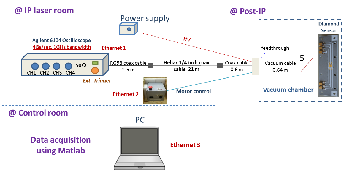
The linear dynamic range of the diamond was demonstrated to be 104, with a lower limit of 103 electrons, which is determined by pickup noise induced by the passage of the beam in the vicinity, and a linear response up to 2107 electrons, which is limited by charge collection saturation effects in the diamond. Since a few thousand electrons is acceptable as background noise for the preliminary halo visualization, emphasis was put on the suppression of the saturation effect for the large signals. In the beam core region, readout becomes nonlinear and the waveform can be strongly distorted both due to space charge inside the diamond crystal bulk and to the instantaneous voltage drop in the 50 resistor, as shown in Fig. 7 (a). The response of the output signal with respect to the charge collected by the DS strip is shown in Fig. 7 (b). The number of electrons striking the diamond can be evaluated according to the beam intensity and transverse beam size, although this can involve some uncertainties, mainly from the determination of the beam size during scans and from instabilities at high intensity.
Rather than reconstructing the waveform based on the charge collection dynamics [28], a ”self-calibration” method was proposed to enable suitable correction of the core profile. The beam core distribution could be measured by the Wire Scanner (WS) located 2.89 m upstream and propagated to the DS to predict the number of electrons striking each strip according to its position with respect to the beam center. Subsequently, the charge which would be collected in the absence of saturation was computed based on the known electron hole pairs generation and charge collection efficiency measured at low incident charge [12]. The rescaling factor was then defined as the ratio of and the charge signal readout, and applied to rescale the DS data within beam core. After such rescaling based on ”self-calibration”, the linear dynamic range could be extended beyond 105 for the populations of collected electrons ranging from to more than . The corrected beam profile is shown in Fig. 8.
III.2 Transverse beam distribution
The transverse beam halo was measured using the DS for various vacuum pressures in the ATF damping ring. Beam intensity was stabilized at 3 /pulse, and the residual gas pressure was increased by switching off SIPs in the arc sections and north straight section of the ATF damping ring.
Measured vertical beam halo distributions, after implementing the rescaling corrections, are consistent with our predictions from tracking simulations, as shown in Fig. 9(a). Moreover, the enhancement of vertical halo for the degraded vacuum pressures is clearly observed. Good agreement between simulations and experiments indicates that the dominant mechanism for vertical halo formation is elastic BGS in the ring.
The measured horizontal beam distributions were also corrected using the described ”self-calibration” method. The reconstructed beam profiles are higher than the predictions from BGS and asymmetrical distributions are observed, with more halo particles on the right side (high energy side), as shown in Fig. 9(b). In addition, the evolution of the beam halo with the vacuum level was found to be negligible, which might be due to insufficient sensitivity, since the background noise level is around 0.01 nC. The DS being located in a high dispersion region after a large horizontal bending magnet ( m), potential non-Gaussian tails in the energy distribution of the beam may also play a role.
IV Emittance Growth from Beam Gas Scattering
Large angle beam-gas scattering events are rare but can induce large betatron oscillation amplitudes, which drive particles beyond the core and into the halo region. Meanwhile, small angle scattering events have higher probability and will act analogously to quantum excitation. They can dilute the core particle distribution and cause emittance growth.
For typical vacuum pressures ( Pa) at ATF, vertical emittance dilution is estimated with the beam distribution function derived in Sec. I and using the Monte Carlo simulation. We assume that the worst vacuum pressure is 3 Pa and the equilibrium vertical emittance (without BGS and IBS) is 12.8 pm. This value is increased to 17.5 pm and 15.5 pm, as predicted by the analytic approximation and Monte Carlo simulation (see Fig. 10), respectively. The difference between the two predictions is due to the approximation of the characteristic function integration in Eq. 19.
To probe the above predictions, measurements of vertical emittance were performed for vacuum pressures ranging from 2.5 Pa to 1.75 Pa. Vertical emittance is evaluated from the beam size measured by an X-ray synchrotron radiation (XSR) monitor and the corresponding function [29]. The observed vertical emittance increases from 12.63 0.46 pm to 16.020.98 pm , which is higher than the simulation result, see Fig. 11(a). The difference might be caused by the uncertainty in the vacuum pressure measurement, the systematic error in the XSR monitor or some other physical process contributing to emittance growth [30]. Moreover, the vertical beam size monitored by the XSR reduces from 7.02 m to 6.2 m when the vacuum pressure recovers from 1.75 Pa to 2.5 Pa, as shown in Fig. 11(b). These pieces of evidence indicate that emittance growth due to BGS is also visible for typical vacuum pressure of Pa and should be taken into account in the design of such a ring.
V Discussion and Conclusions
To explore the primary mechanism of halo formation at ATF, systematic analytical calculations, simulations and experimental measurements have been carried out. We applied formulas to approximate the beam distribution function in the presence of radiation damping, quantum excitation and BGS in the normalized coordinate system. The final simplified formalism, Eq.(15), is solely suitable for the estimation of beam halo, and not the beam core dilution.
For an accurate prediction of the beam distribution distortion, a detailed Monte Carlo simulation was developed in the context of the SAD program. The actual COD and equilibrium beam parameters were approached by introducing local orbit bumps using steering magnets. We attempted to benchmark this simulation using the vacuum lifetime, which was found to be 83 and 87 minutes, from the two numerical methods, respectively, while the measured value was 16 minutes. The presence of additional horizontal beam halo, from sources other than BGS, and the reduction of the transverse acceptance due to nonlinear components may be the reasons for this difference.
To extend the dynamic range of the diamond sensor detector used for the measurements, a rescaling scheme based on ”self-calibration” was proposed and implemented to the DS data. After this rescaling correction, an effective dynamic range of can be achieved. Vertical and horizontal beam halo were measured for several vacuum pressures. For the vertical halo, good agreement between numerical estimations and experimental results for the different vacuum levels is observed. This clearly shows that the vertical halo is dominated by elastic BGS in the ring. On the other hand, the horizontal halo measured by the DS is higher than the BGS prediction and found to be asymmetric. The change in horizontal halo as a function of vacuum pressure is negligible. This shows that BGS has almost no influence on the horizontal halo distribution and other processes (eg. chromaticity, IBS and resonances) may play a more important role.
Simulations and experimental observations of the vertical beam distribution clearly demonstrate that, for typical vacuum pressures in the ATF damping ring, halo generation and emittance growth due to BGS are both visible and significant.
Further studies of beam halo at ATF have been proposed, including the installation of a new OTR/YAG monitor at the dispersion-free region after the extraction from the ring, halo measurements for different kicker timings and optical focusing, and investigation of tails in the momentum distribution.
Acknowledgements.
The authors express their gratitude to the ATF collaboration and to the staff and engineers of ATF. One of us (R. Yang) would like to particularly thank K. Oide for the support and advice on the proper usage of the SAD software, offering suggestions and encouragement. This work was supported by the Chinese Scholarship Council, the Toshiko Yuasa France-Japan Particle Physics Laboratory (project A-RD-10), the France-China Particle Physics Laboratory (project DEV-IHEP-LAL-LC-CEPC) and the MSCA-RISE E-JADE project, funded by the European Commission under grant number 645479.References
- [1] G. Stancari et al., Phys. Rev. Lett. 107, 084802 (2011).
- [2] C. Allen et al., Phys. Rev. Lett. 89, 214802 (2002).
- [3] P. Tenenbaum, T. Raubenheimer, and M. Woodley, in Proceedings of PAC 2001, Chicago, USA, pp. 3843–3845.
- [4] J. Qiang and R. D. Ryne, Phys. Rev. ST Accel. Beams 3, 064201 (2000).
- [5] T. P. Wangler et al., Nucl. Instrum. Methods Phys. Res., Sect. A 519, 425 (2004).
- [6] K. Wittenburg, CERN Accelerator School 2009-005 , pp. 557 (2009).
- [7] J. Yan et al., Nucl. Instrum. Methods Phys. Res., Sect. A 740, 131 (2014).
- [8] K. Hirata and K. Yokoya, Part. Accel. 39, 147 (1992).
- [9] S. Liu, PhD. thesis, Universite Paris-Sud (2015).
- [10] T. Naito and T. Mitsuhashi, in Proceedings of IBIC2015, Melbourne, Australia (2016) pp. 373–376.
- [11] D. Wang et al., Chin. Phys. C 38, 127003 (2014).
- [12] S. Liu et al., Nucl. Instrum. Methods Phys. Res., Sect. A 832, 231 (2016).
- [13] Y. Honda et al., Phys. Rev. Lett. 92, 054802 (2004).
- [14] T. Okugi et al., Phys. Rev. ST Accel. Beams 17, 023501 (2014).
- [15] P. Raimondi and A. Seryi, Phys. Rev. Lett. 86, 3779 (2001).
- [16] G. White et al., Phys. Rev. Lett. 112, 034802 (2014).
- [17] F. Hinode et al., KEK Internal 95 (1995).
- [18] K. Kubo et al., Phys. Rev. Lett. 88, 194801 (2002).
- [19] K. Ohmi, K. Hirata, and K. Oide, Phys. Rev. E 49, 751 (1994).
- [20] T. Raubenheimer, KEK-92-7 (1992).
- [21] S. O. Rice, Bell Labs Technical Journal 23, 282 (1944).
- [22] SAD, is a computer program for accelerator design; see http://acc‑physics.kek.jp/SAD/ .
- [23] K. Kubo, Phys. Rev. ST Accel. Beams 6, 092801 (2003).
- [24] R. Yang et al., J. Phys. Conf. Ser 874, 012063 (2017).
- [25] W. Helmut, Particle Accelerator Physics (Third Edition), pp. 321–329.
- [26] F. Zimmermann et al., SLAC-AP-113 (1998).
- [27] T. Okugi et al., Nucl. Instrum. Methods Phys. Res., Sect. A 455, 207 (2000).
- [28] V. Kubytskyi, S. Liu, and P. Bambade, in Proceedings of IPAC2015, Richmond, USA.
- [29] T. Naito et al., in Proceedings of IBIC2012, Tsukuba, Japan.
- [30] F. Zimmermann, SLAC-AP-107 (1997).