A Topological Approach to Secure Message Dissemination in Vehicular Networks
Abstract
Secure message dissemination is an important issue in vehicular networks, especially considering the vulnerability of vehicle to vehicle (V2V) message dissemination to malicious attacks. Traditional security mechanisms, largely based on message encryption and key management, can only guarantee secure message exchanges between known source and destination pairs. In vehicular networks however, every vehicle may learn its surrounding environment and contributes as a source, while in the meantime act as a destination or a relay of information from other vehicles, message exchanges often occur between “stranger” vehicles. This makes secure message dissemination against malicious tampering much more intricate. For secure message dissemination in vehicular networks against insider attackers, who may tamper the content of the disseminated messages, ensuring the consistency and integrity of the transmitted messages becomes a major concern that traditional message encryption and key management based approaches fall short to provide. However, it is challenging for a vehicle to distinguish which message is true when its received messages from multiple nearby vehicles are conflicting. In this paper, by incorporating the underlying network topology information, we propose an optimal decision algorithm that is able to maximize the chance of making a correct decision on the message content, assuming the prior knowledge of the percentage of malicious vehicles in the network. Furthermore, a novel heuristic decision algorithm is proposed that can make decisions without the aforementioned knowledge of the percentage of malicious vehicles. Simulations are conducted to compare the security performance achieved by our proposed decision algorithms with that achieved by existing ones that do not consider or only partially consider the topological information, to verify the effectiveness of the algorithms. Our results show that by incorporating the network topology information, the security performance can be much improved. This work shed light on the optimum algorithm design for secure message dissemination.
Index Terms:
Vehicular networks, security, message dissemination, decision algorithm.I Introduction
Vehicular networks, with the assistance of dedicated short-range communication (DSRC) [1] and LTE technology, enable safety and non-safety information sharing among vehicles and infrastructure through vehicle to vehicle (V2V) and vehicle to infrastructure (V2I) communications, and therefore are conductive to improving road safety, enhance traffic efficiency and increase comfort and convenience to drivers and passengers [2, 3, 4]. On the other hand, accompanying these benefits brought along by vehicular network applications is the urgent security issue that should be addressed. Specifically, considering the vulnerability of V2V communications, message dissemination in vehicular networks is susceptible to malicious attacks, e.g., malicious vehicles who may spread false messages, tamper or drop the received messages [5] to disrupt delivery of authentic messages. These attacks in vehicular networks could potentially result in catastrophic consequences like city-wide traffic congestion, traffic crash, even loss of lives, and therefore are significant security threats to transportation systems that must be thoroughly investigated before vehicular networks can be deployed.
Vehicular network security design should guarantee authentication, non-repudiation, information integrity, and in some specific application scenarios, confidentiality, to protect the network against attackers [6]. Conventional security mechanisms, largely based on message encryption and key management [7, 8], are effective to guarantee message integrity against outsider attackers, however fall short of protecting the integrity of disseminated messages when there exist insider attackers who possess valid certificates that can pass the authentication process conducted by the certification authorities [9, 10].
To keep the network message dissemination secure against insider attackers, the trustworthiness of each vehicle and the integrity of their transmitted messages are of great importance. Different from traditional security settings, in vehicular networks, information collection and dissemination are conducted by distributed vehicles. Quite often, information may be generated by or received from a vehicle that has never been encountered before. Moreover, the associated vehicular network topology is constantly changing considering that both V2V and V2I connections may emerge opportunistically. These unique characteristics may render the entity-based trust establishment approach, conducted at each vehicle by monitoring their instantaneous neighbours’ behavior, futile in vehicular networks because it is challenging to maintain a stable reputation value for an unknown and fast-moving vehicle. Furthermore, safety-related vehicular network applications usually require vehicles to respond quickly to the received messages [11]. In such cases, determining the integrity of the disseminated messages is of greater importance than the malicious vehicle detection. Therefore, decision algorithms based on data consistency and integrity check emerge, e.g., [12, 13, 14, 15, 16]. However, when a vehicle receives conflicting messages from different nearby vehicles, it is not straightforward to assess which message is true if focusing on data only while ignoring the underlying network topology information that tells where these messages come from. Indeed, messages coming from different paths can be correlated when the these paths share some common nodes. For instance, multiple false messages may result from the same malicious vehicle shared by multiple paths. Therefore, taking the underlying topological information into consideration is essential and beneficial when designing decision algorithms for vehicles to conduct data consistency check.
In this paper, we consider vehicular networks containing insider malicious vehicles that may tamper the content of messages to disrupt their successful delivery. We are interested in investigating topology-based decision algorithms to keep vehicles from being misguided by false messages. To the best of our knowledge, this is the first work that takes the underlying topology information into consideration when checking the consistency of messages for secure message dissemination. Our results shed insight on the optimum decision algorithm design for vehicular networks to improve security performance.
The novelty and major contributions of this paper are summarized as follows:
- 1.
By utilizing the underlying network topology information, we propose two message decision algorithms - the optimum decision algorithm and a heuristic decision algorithm - to cope with the issue of message inconsistency caused by insider malicious vehicles in the network, so as to reduce their impact on the message security performance.
- 2.
The proposed optimum decision algorithm is able to effectively help a vehicle maximally make a correct decision on the content of the message, given the topology information and a prior knowledge of the percentage of malicious vehicles in the network. The proposed heuristic decision algorithm enables a vehicle to make a decision when receiving conflicting messages purely based on topology information, without the need for knowing the percentage of malicious vehicles which can be difficult to estimate in some circumstances.
- 3.
Simulation results show that both our proposed algorithms outperform existing decision algorithms that do not consider or only partially consider the topological information in terms of secure message dissemination in vehicular networks. Besides, the proposed heuristic decision algorithm, which is fairly easy to implement in practice, is sufficient to achieve a high security performance.
The rest of this paper is organized as follows: Section II reviews related work. Section III introduces the system model and the problem formation. The optimum decision algorithm and the heuristic decision algorithm are presented in Section IV and Section V respectively. In Section VI, we conduct simulations to validate the effectiveness of our proposed decision algorithms and discuss their insight. Section VII concludes this paper.
II Related Work
For secure message dissemination in vehicular networks against insider malicious vehicles, the trustworthiness of each vehicle and the integrity of each transmitted message are two major factors need to be considered. Accordingly, three misbehavior detection schemes are commonly adopted to help prevent the disseminated messages from being tampered: entity-centric misbehavior detection scheme, data-centric misbehavior detection scheme, and a combined use of both. In the following, we will review works on these three schemes separately.
Entity-centric misbehavior detection schemes are commonly conducted at each vehicle by monitoring their instantaneous neighbors’ behavior to assess their trustworthiness level, so as to filter out malicious vehicles. In [17], Gazdar et al. proposed a dynamic and distributed trust model based on the use of a Markov chain to evaluate the evolution of each vehicle’s trust value. In [18], Ahmed et al. proposed a trust framework to identify malicious nodes in the network by evaluating the trust value of each vehicle, and the trust includes node trust and recommendation trust. In [19], motivated by the job market signaling model, Haddadou et al. proposed a distributed trust model for vehicular ad hoc networks (VANETs) that is able to gradually detect all malicious nodes as well as boosting the cooperation of selfish nodes. In [20], Sedjelmaci et al. proposed a lightweight intrusion detection framework with the help of a clustering algorithm to overcome the challenges of intermittent and ad hoc monitoring and assessment processes caused by the high mobility and rapid topology change in vehicular networks.
Data-centric misbehavior detection schemes focus on the consistency check of the disseminated data to filter out false data. In [12], Dietzel et al. indicated that redundant data forwarding paths are the most promising technique for effective data consistency check in a multi-hop information dissemination environment, and proposed three graph-theoretic metrics to measure the redundancy of dissemination protocols. In [13], Raya et al. proposed a framework for vehicular networks to establish data-centric trust, and evaluated the effectiveness of four data fusion rules. In [14], Huang et al. firstly demonstrated that information cascading and oversampling adversely affect the performance of trust management scheme in VANETs, and then proposed a novel voting scheme that takes the distance between the transmitter and receiver into account when assigning weight to the trust level of the received data. In [15], Zaidi et al. proposed a rogue node detection system for VANETs utilizing statistical inference techniques to determine whether the received data are authentic. In [16], Radak et al. applied a so-called cautious operator to deal with data received from different sources to detect dangerous events on the road. Their adopted cautious operator is an extension of the Demper-Shafer theory that is known to be superior in handling data coming from dependent sources.
A combined misbehavior detection scheme makes use of both the trust level of vehicles and the consistency of received data to detect misbehaving vehicles and filter out incorrect messages. Works adopting the combined scheme are limited. In [21], Dhurandher et al. proposed a security algorithm using both node reputation and data plausibility checks to protect the network against attacks. The node reputation value is obtained by both direct monitoring and indirect recommendation from neighbors, to detect misbehaving vehicles; and the data consistency check is conducted by comparing the received data with the sensed data by the vehicle’s own sensors. In [22], Li et al. proposed an attack-resistant trust management scheme to evaluate the trustworthiness of both data and vehicles in VANETs. They adopted the Dempster-Shafer theory to combine the data received from different sources, and then used this combined result to update the trust value of vehicles for misbehavior detection.
In summary, all the aforementioned works on protecting vehicular networks from insider attackers either focused on node trust model establishment and management to detect misbehaving nodes in the network, or focused on methods to assess data from different sources to check their consistency, but did not take the underlying network topological information into consideration. Our work distinguishes from theirs in that we focus on the received data itself, and utilize the underlying network topology information to design the decision algorithms for vehicles to check data consistency so as to maximally protect the authenticity of the disseminated messages.
III System Model and Problem Formation
In this section, we first introduce the system model, including the network model, message dissemination model, and the attack model. Then, we give a rigorous description of the research problem addressed in this paper.
III-A Network and Message Dissemination Model
We consider a vehicular network where each vehicle has a unique ID number that is registered in certification authority to represent its identity, and vehicles cannot forge their own or other vehicles’ ID numbers.
Specifically, consider that there is a vehicle in the network (termed as the source vehicle) intending to deliver a message about the road condition to inform other vehicles further away. The road condition information can be abnormal situations, e.g., hazardous road conditions such as traffic accident, slippery road, etc., or normal situation, e.g., uncongested traffic. We assume that the content of message takes value from and represents abnormal road condition and represents normal road condition. It is worth noting that the road situation can also be described as a multi-variable vector and these variables can be correlated [13], e.g., one such variable can be traffic congestion state and another can be accident state. We denote the content of message transmitted by the source vehicle, which represents the actual road condition, by , . Other vehicles do not know the true value of a priori.
The message is forwarded from the source vehicle in a broadcast and multi-hop [23, 24] manner to other vehicles with the help of relay vehicles. Relay vehicles can be any vehicle along the message propagation path. Multi-path forwarding makes it challenging for the attackers to influence all message forwarding paths [12], therefore helps to improve the message security performance of the network. When a vehicle transmits a message to other vehicles, it adds its identity information, i.e., ID number, to the message. This is commonly adopted in vehicular network applications and can be achieved by some standard signature approach [2, 25]. Using this, any vehicle in the network is able to obtain an integrity-protected path list of its received messages recording the relay vehicles of each message, and the records cannot be injected and removed by attackers.
III-B Attack Model
We consider insider attackers in this paper. That is, we assume all vehicles are legitimate vehicles that have passed the authentication process conducted by the certification authority [13, 15]. Vehicles in the network can be classified into two categories: normal vehicles, which behave normally and will forward the received message without any alteration, and malicious vehicles, which may tamper the received message. Malicious vehicles are uniformly distributed in the system with proportion . It follows that the probability of each vehicle being a malicious vehicle is , independent of the event that another distinct vehicle is a malicious vehicle.
Without loss of generality, we assume that the source vehicle is normal and only relay vehicles may be malicious. The normal vehicles do not know which vehicles are normal or malicious. On the other hand, malicious vehicles not only know which vehicles are malicious, but also are capable of communicating with each other via back channels of infinite bandwidth [26]. That is, we assume that malicious vehicles know what the correct message transmitted by the source vehicle is. As a consequence, each malicious vehicle simply transmit the incorrect message, i.e., different from message , to its neighbors. This implies that as long as a message is relayed by at least one malicious vehicle, the message would be incorrect. Fig. 1 gives a simple example of message dissemination process when there are insider attackers in the network.
III-C Problem Formation
Now we give a detailed description of the research problem considered in this paper.
We consider that there is a vehicle, which is several hops away from the source vehicle, trying to make a decision on the message content when it receives several copies of message, and we call it the destination vehicle. Note that the destination vehicle can be any vehicle along the message dissemination path. From the time instant the destination vehicle receives the first message, it waits time period to receive more messages before making a final decision. characterizes the response time requirement on the decision, and a larger potentially allows the vehicle to receive more messages. We will discuss its impact on the integrity of the decision later in the simulation. Let be the number of message received by a destination vehicle during its waiting time period and let be the number of relay vehicles that participate in relaying the copies of message from the source vehicle to the destination vehicle. In the following analysis, we regard and are known to the destination vehicle, which can be readily obtained from the received messages. Consequently, the network being considered has relay vehicles and paths between the source vehicle and the destination vehicle. Other nodes who do not participate in the relay have little impact and hence can be ignored.
Denote the messages received by the destination vehicle by , , , and let the message vector . As each message corresponds to a specific delivery path from the source vehicle to the destination vehicle, we number the corresponding paths by . In addition, we number the relay vehicles by . A vehicle may belong to one or more paths.
Note that due to the existence of malicious vehicles who may tamper the content of the message, the copies of message received by the destination vehicle can be in conflict instead of being consistent with each other. Furthermore, with the potential existence of some shared relay vehicles in different paths, the messages received from different paths may not be independent. These correlations are all contained in the information of message dissemination paths. Therefore, we construct a topology matrix to represent the underlying network topological correlation. Specifically, based on the path information derived from the received messages, the destination vehicle can readily construct a topology matrix , where each row represents a path, each column a node (vehicle), and the -th entry being an indicator whether vehicle belongs to path :
| (1) |
In this paper, we are interested in designing optimal decision algorithms for the destination vehicle to maximize the chance of a correct decision on the content of the disseminated message against attacks from malicious vehicles by utilizing the underlying network topology information. Denote by , the final decision on the content of message made by the destination vehicle. If the decision is the same as the source message, i.e., if , we say the destination vehicle makes a correct decision, otherwise we say it makes an incorrect decision. We use the probability of correct decision, denoted by , as the performance metric to measure the secure message dissemination performance, and can be formally defined as follows:
| (2) |
IV Optimum Decision Algorithm
In this section, we propose a decision algorithm aims to optimize the secure message dissemination performance in terms of maximizing the probability of correct decision , that is,
| (3) |
where is given by (2).
In the following, we will first present the optimum decision algorithm followed by a detailed proof to prove its optimality, and then we will introduce its detailed implementation and discuss its limitation in practical realization.
IV-A Optimum Decision Algorithm
The following theorem summarizes the optimum decision algorithm to maximize .
Theorem 1.
Consider that a destination vehicle receives copies of messages . Given the prior knowledge of the probabilities that the occurrence of abnormal event of interest, e.g., traffic congestion, are , and , which can be estimated from empirical knowledge [27], the optimum decision algorithm that leads to (3) can be shown as follows:
| (4) |
and when , is randomly chosen from 0 and 1 with equal probability.
Proof:
As introduced in [28, 29], the objective of a binary Bayes decision problem is to minimize the expectation of the decision cost, denoted by . Let , , , represents the cost of declaring the final result when actually the source message , and can be negative to represent the benefits of making a correct decision. As a ready consequence of the total probability theorem, the expectation of the decision cost can be expressed as follows:
| (5) |
When assuming and , which is reasonable considering the cost of making an incorrect decision is usually larger than that making a correct decision, the optimum decision algorithm that minimizes the expectation of the decision cost made by the destination vehicle given its copies of received message , is given by [29]:
| (6) |
where and are the two conditional probabilities of the occurrence of event , which characterize the correlations between received messages. Besides, when a tie occurs, namely, when , is randomly chosen from and 1 with equal probability.
From (5), when assuming the cost of making a correct decision is and making an incorrect decision is , namely, by assuming and , we have:
| (7) |
It follows that a minimization of the expectation of the decision cost, is equivalent to a maximization of the probability of correct decision, namely, we have
| (8) |
Therefore, the optimum decision algorithm for the optimization problem (3) is exactly the decision algorithm that provides a solution to the classical Bayes decision problem in a special case, shown as (4), which finalize the proof. ∎
Remark 2.
It can be seen from (4) that, given the probabilities of the occurrence of abnormal event of interest, and respectively, the decision on or depends on the ratio . That is, given a set of received messages , the destination vehicle need to calculate the probability that the event occurs if the true message is 1, denoted as , and the probability that the event occurs if the true message is 0, denoted as . A decision on is then made by comparing the value of and . Therefore, calculation of the two probabilities is the critical part of implementing the algorithm in practice.
In summary, the optimum decision algorithm for the destination vehicle to maximally make a correct decision on the message content works as detailed in Algorithm 1, where the details of calculating the two terms and will be given in the following subsection.
- INPUT:
, , ,
- OUTPUT:
- begin
- 1.
Construct topology matrix based on the paths information derived from the received copies of message;
- 2.
Calculate and according to (12) and () respectively, given the network topology information and a prior knowledge on the proportion of malicious vehicles in the network;
- 3.
If then
elseif then ;
else then is randomly chosen from and with equal probability;
end
- end
IV-B Algorithm Implementation
In this part, we will introduce the detailed implementation of the proposed optimum decision algorithm. As discussed in Remark 2, the first step is to calculate the two probabilities and as they are prerequisite to obtaining the final decision .
The main idea behind the calculation of and is as follows. We classify vehicles into three different types based on the paths they belong to. We call a vehicle a Type 0 (or Type 1) vehicle if it only belongs to paths that deliver messages with content 0 (or 1) to the destination vehicle, and a vehicle is a Type 2 vehicle (if any) if it belongs to at least one path that delivers message with content 0 and another path that delivers message with content 1 to the destination vehicle. That is a Type 0 vehicle only belongs to paths that deliver consistent messages 0; a Type 1 vehicle only belongs to paths that deliver consistent messages 1; while a Type 2 vehicle belong to paths that delivers inconsistent messages. Therefore, by separating the paths according to the delivered message contents, the conclusion readily follows that given , all the Type 1 and Type 2 vehicles are normal vehicles, meanwhile malicious vehicles only exist among Type 0 vehicles. Then, by listing and analyzing all the different combination of malicious vehicles among the Type 0 vehicles, we can obtain the result of our target conditional probability . The idea of calculating is totally the same.
In the following, we will first demonstrate the method of constructing topology matrix based on the above idea, and then calculate the two probabilities and respectively. Without loss of generality, we assume that among the copies of messages received by the destination vehicle, there are exactly , messages with content and the other messages with content . Note that and are both trivial cases implying no conflict in the received messages so that the decision is straightforward, therefore we only consider the case when .
1 Constructing the topology matrix
Specifically, recall the definition of the topology matrix given in (1), that each row corresponds to a path and each column corresponds to a vehicle. Based on the idea discussed above to calculate the probabilities and , we re-arrange the network topology matrix in the following form:
| (9) |
where , , and , if exist, are non-zero matrices, and is a sub-matrix corresponding to the paths that deliver messages with content 1 to the destination vehicle, and is a sub-matrix corresponding to the paths that deliver messages with content 0 to the destination vehicle. Besides, the columns of and correspond to vehicles that only belong to paths that deliver messages with content 1 and that deliver messages with content 0 to the destination vehicle respectively, i.e., Type 1 vehicles and Type 0 vehicles respectively. The columns of sub-matrix correspond to all the Type 2 vehicles. Assume that the number of Type and Type vehicles are and respectively, , and the number of Type 2 vehicles is . It follows that matrices and are of size and respectively, and the matrix is of size .
It is worth noting that the above arrangement of columns and rows of matrix corresponds to a re-numbering of vehicles and paths and it does not change the underlying topology in terms of paths information. Besides, the sub-matrix can be non-existent if , i.e., when the paths that deliver messages 0 to the destination vehicle contains all the vehicles in the network. Under this circumstance, . Similarly, the sub-matrix (or ) can also be non-existent when (or .
2 Calculation of and
In this part, we show the method of calculating the two conditional probabilities and using the constructed topology matrix . The following two theorems summarize the results.
Theorem 3.
Consider that a destination vehicle receives copies of message , and among which messages are with content and the other messages are with content 0, . Conditioned on the source message , the conditional probability of the occurrence of event can be calculated as follows:
| (10) |
where is the number of vehicles that only belong to paths that deliver messages with content 0 to the destination vehicle, i.e., the number of Type 0 vehicles in the network, and is the number of combinations that contain exactly malicious Type 0 vehicles leading to the occurrence of event .
Proof:
When , there are no Type 0 vehicles in the network, which implies that the paths that deliver messages with content to the destination vehicle contain all the vehicles in the network, and the topology matrix . Under this circumstance, conditioned on the source message , when the event that messages are with content 1 occurs, all the vehicles in the network should be normal vehicles. It follows that the event that the other messages are with content 0 occurs with probability 0. Therefore, we have when .
When , from the topology matrix , we can conclude that if the matrix exists, then the corresponding Type 2 vehicles should be all normal vehicles. Observing that there is no possibility for two paths sharing the same malicious vehicle to deliver different contents. Therefore, malicious vehicles exist either among Type 1 vehicles or among Type 0 vehicles.
Given the source message , all the Type 1 vehicles should be normal vehicles. Malicious vehicles can only exist among Type 0 vehicles. Besides, the malicious Type 0 vehicles should be able to compromise all the paths (corresponding to the sub-matrix ) to cause the occurrence of the event that all the paths delivering messages with incorrect content . Therefore, any combination of malicious vehicles should satisfy the follows condition: by implementing element-wise union on their corresponding columns in sub-matrix , i.e., implementing element-wise Boolean operation OR on them, the result should be a column with each entry be .
Note that the number of malicious type 0 vehicles can be any integer within . We denote by event that randomly choosing columns from sub-matrix and then conducting element-wise union operation to them, there results a column with each entry being . Denote by the total number of combinations that event occurs. Therefore, we have
| (11) |
where , and is an indicator function that when is true; otherwise .
It then follows from the combination theory [30] that :
| (12) |
where the first part corresponds to the probability that the paths deliver messages with correct content , so that all the vehicles contained in these paths are therefore normal vehicles; and the second part is the probability that the paths deliver messages with incorrect content , which summing up all the probabilities of different malicious vehicle combinations. ∎
Theorem 4.
Consider that a destination vehicle receives copies of message , and among which messages are with content and the other messages are with content 0, . Conditioned on the source message , the conditional probability of the occurrence of event can be calculated as follows:
| (13) |
where is the number of vehicles that only belong to paths that deliver messages with content 1 to the destination vehicle, i.e., the number of Type 1 vehicles in the network, and is the number of combinations that exactly malicious Type 1 vehicles leading to the occurrence of event .
Denote by event that randomly choosing columns from sub-matrix and then conducting element-wise union operation to them, there results a column with each entry be . Denote by the total number of combinations that event occurs. Then we have
| (14) |
where . Therefore, this theorem can be readily proved following the same method as that used in the proof of Theorem 3, and hence is ignored.
IV-C Discussion
From the analysis in Section IV-B, we can see that the value of , , and , in (10), , in (13) can be obtained from the network topology matrix. That is, when the received messages , and the network topology is given, the value of , , , , and , are all determined. However, the exact values of and , shown also in (10) and (13), also depend on the proportion of malicious vehicles in the network, which usually, is not easy to be obtained or estimated as a prior knowledge. In the following, we use a simple example to show the dependency on of the proposed optimum decision algorithm.
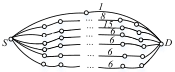
Consider a network that contains a total of independent paths from the source vehicle to the destination vehicle. The first three paths, containing and vehicles respectively deliver messages with content to the destination vehicle, and the other four paths, containing vehicles each, deliver messages with content to the destination vehicle. See Fig. 2 for an illustration.
According to (10) and (13), we have:
| (15) |
and
| (16) |
Therefore,
| (17) |
Let
| (18) |
and
| (19) |
and plot them with different values of , see Fig. 3 for an illustration. We can see that the value of depends on the percentage of malicious vehicles in the network. Specifically, it is shown in Fig. 3 that when is smaller than a threshold, e.g., in this case, the value of is smaller than , while when is larger than the threshold, the value of is larger than , and will further increase with an increase of . Therefore, given the network topology, the optimum decision based on (4) relies on the value of . This illustrates that the value of is indispensable in adopting the optimum decision algorithm to achieve an accurate decision result.
V Heuristic Decision Algorithm
As discussed in the Section IV-C, the implementation of the optimum decision algorithm proposed in the last section relies on prior knowledge of the percentage of malicious vehicles in the network, which is usually not easy to be obtained or estimated. In this section, to eliminate the dependence on , we propose a heuristic decision algorithm for the destination vehicle to make a decision when receiving conflicting messages purely based on network topology information only.
The heuristic decision algorithm is derived from the principle of Maximum Likelihood Estimation [31], which can be described as follows:
| (20) |
where are the messages received by the destination vehicle, is the source message and is the decision made by the destination vehicle. When , is randomly chosen from 0 and 1 with equal probability.
Based on the received messages , , , and the path information obtained from messages, the method of constructing the topology matrix is the same as introduced in Section IV-B, i.e., . Therefore, by combining (10), (13) and (20), it is ready to have , and when and ,
| (21) |
Recall that both sub-matrix and correspond to a sub-network of the considered network and the common nodes shared by the two sub-networks (if any) can not be malicious vehicles. Therefore, when considering the potential malicious vehicle combinations, we avoid these common nodes and only focus on the sub-matrix and . Specifically, we regard the network corresponding to sub-matrix and as networks that each row represents a complete path and each column represent a vehicle, denoted by and respectively. In the following, with a twist of the vertex-cut [32] terminology from graph theory which defines a vertex set whose removal would disconnect the graph, we define malicious cut set, size of a malicious cut set, and minimal malicious cut set of a network in this paper, and demonstrate that the parameter , and , in (21), which was defined in (11) and (14), are exactly the number of malicious cut sets with size of the network and respectively.
Definition 5.
A malicious cut set of a network is a combination of vehicles, where if all vehicles in the set are malicious vehicles all paths of the network can be compromised. The size of a malicious cut set is the number of vehicles contained in the set. A minimal malicious cut set is a malicious cut set with the smallest size.
It is worth noting that the network may have multiple malicious cut sets and multiple minimal malicious cut sets. Consider the network shown in Fig. 4 for an example. Vehicle sets , , and (to name a few) are all malicious cut sets of the network, and a minimal malicious cut set is the malicious cut set with size . Therefore, to compromise all paths of this network, the minimum number of malicious vehicles needed is .
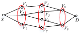
Based on Definition 5, if a vehicle set is a malicious cut set, then each path of the network contains at least one vehicle belongs to this set. Recall that (or ) represents the number of combinations that randomly choosing columns from sub-matrix ( and then conducting element-wise union to them, there results a column with each entry be . That is, (or ) represents the number of combinations that by choosing vehicles from Network (or ) to form a vehicle set, each path of network (or ) contains at least one vehicle belongs to this set. Therefore, , and , are exactly the number of malicious cut sets with size of the network and respectively.
According to the properties of malicious cut sets, it can be readily obtained that if , and , if . Similarly, we have if , and , if .
Define
| (22) |
and
| (23) |
the smallest integer that satisfies and respectively. Therefore, is the size of the minimal malicious cut set of network , and is the number of minimal malicious cut sets of network . Similarly, is the size of the minimal malicious cut set of network , and is the number of minimal malicious cut sets of network . This follows that
| (24) |
where the first step is obtained from the fact that , , and , , and the second step is obtained by only keeping the first item of both the numerator and denominator. Considering the fact that when is small, the probability that there are malicious vehicle in the network is much smaller than the probability that there are malicious vehicles in the network, therefore, this approximation is quite accurate.
Note that when is small, we have . Therefore, when , whether the value of shown as (24) is larger than is dominantly determined by the value of . Specifically, when , we have . In this case, the coefficient plays marginal role and therefore ; when , we have , and therefore . On the contrary, when , whether the value of is larger than would heavily depend on the value of the coefficient . Consequently, we have
| (25) |
which shows that to compare the values of and , we only need to compare the values of and , namely, the size of minimal malicious cut set of network and when , or the value of and , namely, the number of minimal malicious cut sets of network and when they have the same size of minimal malicious cut set.
From Menger’s Theorem [32], the size of the minimal vertex-cut whose removal would disconnect two non-adjacent vertices, is equal to the maximum number of vertex-independent paths between these two non-adjacent vertices. Therefore, it can be concluded that the size of minimal malicious cut set of a network is also equal to the maximum number of node-disjoint paths in the network between the source vehicle and the destination vehicle. Therefore, and are also the numbers of maximum number of node-disjoint paths exist in network and respectively. Note that calculating the maximum number of vertex-disjoint paths from source to destination is a special case of finding the maximum flow problem by setting every vertex capacity [32]. Therefore, the values of and can be readily obtained by existing maximum flow algorithms, e.g., introduced in [32, 33, 34]. When , and can be obtained by exhaustive search algorithm according to their definitions given by (11) and (14).
In summary, by combining (20) and (25), the decision rule of our proposed heuristic algorithm can be shown as
| (26) |
and when , and , is randomly chosen from and with equal probability.
Remark 6.
It is worth noting that in the above analysis, the network with a topology matrix may not be unique. For instance, a topology matrix can correspond to both networks shown in Fig. 5. However, the malicious cut sets of the networks with different topology remain the same as there is a one-to-one correspondence between each malicious cut set and a combination of columns from the topology matrix that an element-wise union of them resulting in a column with each entry being 1. That is, as long as networks have the same topology matrix , they would have the same malicious cut sets. Therefore, the network (or ) corresponding to the same sub-matrix (or ) may not unique, however it does not affect their malicious cut sets analysis.
Remark 7.
The implication of the heuristic decision algorithm (26) can also be explained straightforwardly as follows. Given two networks that deliver conflicting message contents, by removing the common nodes shared by these two networks and regarding each path after the removal of the common nodes as a new complete path, there results in two new independent networks that deliver conflicting message contents. Therefore, decision can be made by comparing the robustness of the two new networks. Note that a smaller size of the minimal malicious cut set of a network implies a less number of minimal malicious vehicles are required to compromise that network, and consequently, a higher probability to deliver incorrect messages. Therefore, the decision will always be chosen as the message delivered by the network with a lower probability to be compromised.
From (26), we can see that the decision result is now entirely determined by the network topology, and is independent of the proportion of malicious vehicles in the network. That is, the proposed heuristic decision algorithm is purely topology-based so that is easy to be implemented in practice. In summary, the heuristic decision algorithm works as detailed in Algorithm 2.
- INPUT:
- OUTPUT:
- begin
- 1.
Construct topology matrix based on the paths information derived from the received copies of message;
- 2.
Based on the constructed topology matrix , calculate and based on maximum flow algorithm;
- 3.
- end
VI Simulation and Discussion
In this section, we conduct simulations to establish the validity of the decision algorithms proposed in Section IV and Section V. We generate a network that vehicles are Poissonly distributed in the road with density , and each relay vehicle has a probability to be a malicious vehicle. Vehicles communicate with their neighbors adopting the unit disk model [23, 35] with transmission range m [36]. We focus on a destination vehicle located at a distance from the source vehicle. From the time instant the destination vehicle receives the first message reporting road condition, it waits time period to receive more number of messages before it starts to make a decision. The per-hop transmission delay is assumed to be ms [36]. For the road condition, we choose a rather conservative probability of the occurrence of an abnormal situation. Specifically, we set that an hazardous road/environmental condition happens randomly with probability [13], i.e., we set and .
At each simulation, a topology matrix can be constructed based on the underlying network topology. Therefore, given the malicious vehicle distribution and the topology information, the content of the messages received by the destination vehicle is determined. The destination vehicle then makes a decision given the received messages and the derived underlying topology information according to our proposed decision algorithms at each simulation. The decision result can be either correct or incorrect. The simulation is repeated 5000 times and the proportion of the correct decision, i.e., the probability of correct decision, is plotted.
In the following, we first compare our proposed two decision algorithms, and then we study the effects of topology information, and some performance-impacting parameters on the algorithms. The performance-impacting parameters including the proportion of malicious vehicle in the network, the choice of waiting time by the destination vehicle before it starts to make the decision..
VI-A Comparison of the two proposed algorithms
In this part, we compare the message security performance achieved by the two proposed decision algorithms to provide insight on the optimum decision algorithm design for secure message dissemination.
Fig. 6 compares the probability of correct decision achieved by the proposed optimum decision algorithm (labeled as Optimum Algorithm) and by the proposed pure topology-based heuristic decision algorithm (labeled as Heuristic Algorithm) respectively. It is shown that when the percentage of malicious vehicles in the network is small, e.g., when in this case, the message security performance achieved by the optimum decision algorithm is only slightly better than the performance achieved by the heuristic decision algorithm. This implies that the heuristic decision algorithm, that purely based on network topology information and easily to be implemented in practice, is sufficient to achieve a high message security performance for vehicular networks.
VI-B Impact of topology information
To evaluate the effectiveness of our proposed algorithms that takes the underlying topology information into consideration, we compare the security performance, in terms of the probability of correct decision made by the destination vehicle, achieved by our proposed algorithms described by Algorithm 1 and 2 respectively, with that achieved by existing weighted voting algorithms like the weighted voting algorithm proposed in [29] (labeled with WV: MMSE) that considers partial correlation between messages, the weighted voting algorithm proposed in [14] (labeled with WV: that does not consider the underlying topology information causing the correlation between messages, and the majority voting (a special case of weighted voting by assigning identical weights to each vote) that totally ignores the underlying topological correlation. Specifically, the weighted voting algorithm proposed in [29] set weight to each message as , where is the error covariance matrix whose th entry is defined by the error covariance between message and message , calculated by . is the inverse matrix of the error covariance matrix and is the th entry of the matrix . The weighted voting algorithm proposed in [14] simply assigns weight to each message as , where is a weighting factor to reduce the oversampling impact caused by messages generated from the same source and is the number of hops travelled by the th message from the source to the destination.
It can be seen in Fig. 7 that both our proposed algorithms outperform the weighted voting algorithms proposed in [29], [14] and the majority voting algorithm, which demonstrates that our algorithms taking into account topology information and correlation between different copies of message are able to effectively improve the robustness of vehicle networks against attacks from malicious vehicles.
VI-C Impact of the percentage of malicious vehicles
Fig. 7 reveals the relationship between the probability of correct decision and the percentage of malicious vehicles in the network, . It can be seen that the probability of correct decision made by the destination vehicle decreases to its minimum value when the proportion of malicious vehicles in the network is larger than a certain threshold. Beyond that threshold, a further increase in has little impact on the security performance. Specifically, as shown in Fig. 7, when is small, the security performance achieved assuming the optimum decision algorithm decreases with an increase of ; however, when increases beyond a certain threshold, a further increase in has no impact on the security performance. This can be explained by the fact that the more malicious vehicles in the network, the more tampered copies of message will be delivered, and therefore a lower chance for the destination vehicle to make a correct decision regardless of what algorithm it adopts. Furthermore, when the number of malicious vehicles in the network reaches a certain threshold, most of the message dissemination paths will be compromised. In this case, the destination vehicle will totally misguided by the incorrect messages and the message security performance approaches its minimum value .
VI-D Impact of the waiting time period
As mentioned in Section III-C, the waiting time period the destination vehicle waits before it starts to make a decision is an important parameter that should balance the trade-off between the response time requirement and the integrity of the decision. Therefore, in this part, we study the impact of the waiting time period on the security performance assuming the two proposed algorithms, under different traffic densities.
Fig. 8 demonstrates the relationship between the probability of correct decision, , and the waiting time period the destination vehicle waits before it starts to make a decision, assuming our two proposed algorithms respectively, and gives insight into the choice of waiting time by the destination vehicle. Importantly, we can see that for both algorithms, a larger number of waiting time is beneficial to the secure message dissemination because a longer waiting time potentially implies a larger number of received messages. This consequently, brings more information on the underlying network topology, and therefore leads to a more robust result of the data consistency check. However, when increases beyond a certain threshold , e.g., in the case of =0.01veh/m, when adopting the proposed optimum decision algorithm and when adopting the proposed heuristic decision algorithm when, a further increase in has marginal (less than ) impact on the probability of correct decision. This is due to the fact that when is larger than a threshold, the marginal return brought by waiting a longer time to the security performance is diminishing. Furthermore, it can be seen that to achieve the same message security performance, when the vehicular density is lower, the waiting time needs to be longer. Therefore, when determining the waiting time period, it is important to take the vehicular density into account, e.g., in areas where the vehicular density is large, the waiting time can be reduced. Thus, Fig. 8 exhibits a guide on the choice of waiting time period for destination vehicles.
VII Conclusions
This paper proposed two decision algorithms that utilizes the underlying network topology information to address the issue of message inconsistency caused by malicious vehicles that would tamper the content of disseminated messages. The optimum decision algorithm proposed is able to maximally help a destination vehicle make a correct decision on the message content, based on the network topology information and a prior knowledge of the percentage of malicious vehicles in the network. The heuristic decision algorithm proposed enables a vehicle to make a decision purely based on network topology information, therefore is easier to implement in practice. Simulations were conducted to verify the effectiveness of the algorithms. We demonstrated that the heuristic decision algorithm is able to achieve a security performance close to that achieved by the optimum decision algorithm, especially when the percentage of malicious vehicles in the network is small. By comparing the two proposed algorithms with existing algorithms that do not consider the underlying topological information or only partially consider message correlation, we showed that our proposed algorithms greatly outperform existing ones. Moreover, we discussed the impact of some key parameters on the performance of the proposed algorithms, including the percentage of malicious vehicles in the network, and the waiting time the destination vehicle waits before making the final decision. Our results give insight on the optimum decision algorithm design for vehicular networks to improve message security.
References
- [1] J. B. Kenney, “Dedicated Short-Range Communications (DSRC) Standards in the United States,” Proc. IEEE, vol. 99, no. 7, pp. 1162-1182, 2011.
- [2] M. A. Javed, E. B. Hamida, “On the Interrelation of Security, QoS, and Safety in Cooperative ITS”, IEEE Trans. Intell. Transp. Syst., vol. 18, no. 7, pp 1943 - 1957, Jul. 2017.
- [3] J. E. Siegel, D. C. Erb, and S. E. Sarma, “A Survey of the Connected Vehicle Landscape–Architectures, Enabling Technologies, Applications, and Development Areas”, to appear in IEEE Trans. Intell. Transp. Syst., 2017.
- [4] K. Zheng, et al., “Heterogeneous Vehicular Networking: A Survey on Architecture, Challenges, and Solutions,” IEEE Commun. Surveys Tuts., vol. 17, no. 4, pp. 2377-2396, Fourth Quarter, 2015.
- [5] E. Fonseca and A. Festag, “A survey of existing approaches for secure ad hoc routing and their applicability to VANETs,” NEC Network Laboratories, Heidelberg, Germany, NEC Tech. Rep. NLE-PR-2006-19, Version 1.1, Mar. 2006.
- [6] J. Sun, C. Zhang, Y. Zhang, Y. Fang, “An Identity-Based Security System for User Privacy in Vehicular Ad Hoc Networks”, IEEE Trans. Parallel Distrib. Syst., vol. 21, no. 9, pp. 1227 - 1239, Sep. 2010.
- [7] H. Tan, M. Ma, H. Labiod, A. Boudguiga, J. Zhang, and P. H. J. Chong, “A secure and authenticated key management protocol (SA-KMP) for vehicular networks,” IEEE Trans. Veh. Technol., vol. 65, no. 12, pp. 9570–9584, Dec. 2016.
- [8] J. Petit, F. Schaub, M. Feiri, F. Kargl, “Pseudonym Schemes in Vehicular Networks: A Survey”, IEEE Commun. Surveys Tuts., vol. 17, no. 1, pp. 228-255, First Quarter, 2015.
- [9] Q. Yang, H. Wang, “Toward trustworthy vehicular social networks”, IEEE Commun. Mag., vol. 53, no. 8, pp, 42 - 47, Aug. 2015.
- [10] S. Dietzel, R. Heijden, H. Decke and F. Kargl, “A flexible, subjective logic-based framework for misbehavior detection in V2V networks”, in Proceeding of IEEE WoWMoM, 2014.
- [11] Y. Du, M. Chowdhury, M. Rahman, K. Dey, A. Apon, A. Luckow, L. B. Ngo, “A Distributed Message Delivery Infrastructure for Connected Vehicle Technology Applications”, to appear in IEEE Trans. Intell. Transp. Syst., 2017.
- [12] S. Dietzel, J. Petit, G. Heijenk, and F. Kargl, “Graph-Based Metrics for Insider Attack Detection in VANET Multihop Data Dissemination Protocols,” IEEE Trans. Veh. Technol., vol. 62, no. 4, pp. 1505-1518, May. 2013.
- [13] M. Raya, P. Papadimitratos, V. D. Gligor, and J. P. Hubaux, “On Data-Centric Trust Establishment in Ephemeral Ad Hoc Networks,” in IEEE INFOCOM, 2008.
- [14] Z. Huang, S. Ruj, M. A. Cavenaghi, M. Stojmenovic, and A. Nayak, “A social network approach to trust management in VANETs,” Peer-to-Peer Networking and Applications, vol. 7, no. 3, pp. 229-242, 2014.
- [15] K. Zaidi, M. B. Milojevic, V. Rakocevic, A. Nallanathan, and M. Rajarajan, “Host-Based Intrusion Detection for VANETs: A Statistical Approach to Rogue Node Detection,” IEEE Trans. Veh. Technol., vol. 65, no. 8, pp. 6703-6714, Aug. 2014.
- [16] J. Radak, B. Ducourthial, V. Cherfaoui, and S. Bonnet, “Detecting Road Events Using Distributed Data Fusion: Experimental Evaluation for the Icy Roads Case,” IEEE Trans. Intell. Transp. Syst., vol. 17, no. 1, pp. 184-194, Jan. 2016.
- [17] T. Gazdar, A. Rachedi, A. Benslimane, and A. Belghith, “A distributed advanced analytical trust model for VANETs,” in IEEE GLOBECOM 2012.
- [18] S. Ahmed, S. Al Rubeaai, and K. Tepe, “Novel Trust Framework for Vehicular Networks”, IEEE Trans. Veh. Technol., vol. 66, no. 10, pp. 9498 - 9511, Oct. 2017.
- [19] N. Haddadou, A. Rachedi, and Y. Ghamri-Doudane, “A Job Market Signaling Scheme for Incentive and Trust Management in Vehicular Ad Hoc Networks,” IEEE Trans. Veh. Technol., vol. 64, no. 8, pp. 3657-3674, Aug. 2015.
- [20] H. Sedjelmaci, and S. M. Senouci, “An accurate and efficient collaborative intrusion detection framework to secure vehicular networks”, Computers and Electrical Engineering, vol. 43, pp. 33-47, 2015.
- [21] S. K. Dhurandher, M. S. Obaidat, A. Jaiswal, A. Tiwari and A. Tyagi, “ Vehicular Security Through Reputation and Plausibility Checks,” IEEE Syst. J., vol. 8, no. 2, pp. 384 - 394. Jun. 2014.
- [22] W. Li, and H. Song, “ART: An Attack-Resistant Trust Management Scheme for Securing Vehicular Ad Hoc Networks,” IEEE Trans. Intell. Transp. Syst., vol. 17, no. 4, pp. 960-969, Apr. 2016.
- [23] G. Mao and B. D.O. Anderson, “Graph Theoretic Models and Tools for the Analysis of Dynamic Wireless Multihop Networks”, in IEEE WCNC, pp. 1-6, 2009.
- [24] J. Ma, F. Le, A. Russo, J. Lobo, “Detecting distributed signature-based intrusion: The case of multi-path routing attacks”, in IEEE Conference on Computer Communications (INFOCOM), 2015.
- [25] S. Dietzel, J, Gurtler, R. Heijden and F. Kargl, “Redundancy-based statistical analysis for insider attack detection in VANET aggregation schemes”, in IEEE VNC, 2014.
- [26] J. Ponniah, Y. C. Hu and P. R. Kumar, “A Clean Slate Approach to Secure Ad Hoc Wireless Networking - Open Unsynchronized Networks”, IEEE Trans. Control Netw. Syst., vol. 4, no. 1, pp. 37 - 48, March, 2017.
- [27] Y. Wang, H. Ieda, and F. Mannering, “Estimating Rear-End Accident Probabilities at Signalized Intersections: Occurrence-Mechanism Approach”, Journal of Transportation engineering, vol. 129, no. 4, Jul. 2003.
- [28] M. Kam, Q. Zhu and W. S. Gray, “Optimal data fusion of correlated local decisions in multiple sensor detection systems”, IEEE Trans. Aerosp. Electron. Syst, vol. 28, no. 3, pp. 916-920, Jul. 1992.
- [29] Y. Zhu, Multisensor Decision and Estimation Fusion, United States, Springer, 2003.
- [30] W. Feller, An Introduction to Probability Theory and Its Applications, vol. 2. New York, NY, USA: Wiley, 1971.
- [31] M. H. DeGroot, and M. J. Schervish, Probability and statistics, fourth edition, Boston, MA: Addison-Wesley, 2002.
- [32] J. L. Gross, and J. Yellen, Graph theory and its applications, second edition, Boca Raton, Florida, USA, Chapman & Hall/CRC, 2006.
- [33] D. R. Karger and C. Stein. A new approach to the minimum cut problem. J. ACM, vol. 43, no. 4, pp. 601–640, Dec. 1996.
- [34] A. V. Goldberg and R. E. Tarjan. A new approach to the maximum-flow problem. J. Assoc. Comput. Mach., vol. 35, no. 4, pp. 921–940, Oct. 1988.
- [35] Y. Wang, J. Zheng, and N. Mitton, “Delivery Delay Analysis for Roadside Unit Deployment in Vehicular Ad Hoc Networks with Intermittent Connectivity”, IEEE Trans. Veh. Technol., vol. 65, no. 10, pp. 8591 - 8602, Oct. 2016.
- [36] Z. Zhang, G. Mao, and B. D. O. Anderson, “Stochastic Characterization of Information Propagation Process in Vehicular Ad hoc Networks,” IEEE Trans. Intell. Transp. Syst., vol. 15, no. 1, pp. 122-135, Feb. 2014.
| Jieqiong Chen (S’16) received the Bachelor’s degree in Engineering from Zhejiang University, Zhejiang, China, in 2012, and she is currently working toward the Ph.D. degree in engineering at the University of Technology Sydney, NSW, Australia. Her research interests include wireless communications and optimum vehicular network design for intelligent transporatation systems. |
| Guoqiang Mao (S’98-M’02-SM’08-F’17) joined the University of Technology Sydney in February 2014 as Professor of Wireless Networking and Director of Center for Real-time Information Networks. Before that, he was with the School of Electrical and Information Engineering, the University of Sydney. He has published about 200 papers in international conferences and journals, which have been cited more than 5000 times. He is an editor of the IEEE Transactions on Wireless Communications (since 2014), IEEE Transactions on Vehicular Technology (since 2010) and received “Top Editor” award for outstanding contributions to the IEEE Transactions on Vehicular Technology in 2011, 2014 and 2015. He is a co-chair of IEEE Intelligent Transport Systems Society Technical Committee on Communication Networks. He has served as a chair, co-chair and TPC member in a large number of international conferences. He is a fellow of IEEE and IET. His research interest include intelligent transport systems, applied graph theory and its applications in telecommunications, Internet of Things, wireless sensor networks, wireless localization techniques and network performance analysis. |
| Changle Li (M’09–SM’16) received the Ph.D. degrees in communication and information system from Xidian University, China, in 2005. Since then, he conducted his postdoctoral research in Canada and the National Institute of information and Communications Technology (NICT), Japan, respectively. He has been a visiting scholar at the University of Technology Sydney (UTS) and is currently a Professor with the State Key Laboratory of Integrated Services Networks, Xidian University. He is an IEEE Senior Member and his research interests include intelligent transportation systems, vehicular networks, mobile ad hoc networks, and wireless sensor networks. |
| De-gan Zhang (M’01) Born in 1970, Ph.D. Graduated from Northeastern University, China. Now he is professor of Tianjin Key Lab of Intelligent Computing and Novel software Technology, Key Lab of Computer Vision and System, Ministry of Education, Tianjin University of Technology, Tianjin, 300384, China. His research interest includes IOT, WSN, IOV, etc. His E-mail: gandegande @126.com. He is the corresponding author of this paper. |