Construction of low-dimensional system reproducing low-Reynolds-number turbulence by machine learning
Abstract
In a dissipative system, there exists the (global) attractor which has finite fractal dimensions. The flow on the attractor can be parametrized by a finite number of parameters (Temmam 1987). Using machine learning we demonstrate how to construct precise low-dimensional governing equations which are valid in some range of Reynolds number for low-Reynolds-number turbulence in plane Couette flow.
In a dissipative system it is expected that a final flow state (attractor) is enclosed in a subspace whose dimension is much lower than the dimension of the system [1]. If the attractor has the Hausdorff dimension , then many projectors of dimension are injective on [2], where [] is Gauss’ symbol. This means that if each point of the attractor has finite thickness only in low number of directions, then the flow state can be decided using small number of variables, and there exists an exactly low-dimensional system. In this paper we use machine learning to build a high-precision low-dimensional system for early-stage turbulence in transitional plane Couette flow.
Let us consider plane Couette flow. The non-dimensionalized governing equations, incompressible Navier–Stokes equations, and boundary conditions are
| (1) | ||||
| (2) | ||||
| (3) | ||||
| (4) |
where the coordinates, , and , are taken respectively in the streamwise, wall-normal and spanwise directions, is a unit vector in the direction, and denotes the Reynolds number based on half the wall separation and half the wall speed difference. The same symmetry as Kreilos and Eckhardt(2012)[3],
| (5) |
is imposed on the flow.
We now construct a low-dimensional system on an attractor using variables. As a training set we use the orbit on an attractor obtained from DNS (direct numerical simulation) for the Navier–Stokes equations, and then the evolution of the orbit is predicted by a low-dimensional system constructed, using multiple regression analysis, as
| (6) |
where is an -dimensional mapping function, and () represents discretized time with increment of unity. Variables () are taken to be spatially averaged physically important quantities, such as total kinetic energy, total enstrophy, and so on, to be used as arguments of multiple regression analysis. We employ the function kqr (kernal quantile regression)[4] in the package Kernlab[5], which can be used in R, to perform multiple regression analysis precisely. We take default parameters of kqr except for the regularization parameter . We set the value of in the range .
Figure 1 shows the onset of chaos (turbulence) as a consequence of bifurcations, i.e. the appearance of Nagata’s steady solution from the saddle-node bifurcation at , the bifurcation of the periodic solution from the upper branch of the Nagata solution, and subsequent period doubling cascades. This is the reproduction of the figure in Kreilos and Eckhardt (2012)[3]. Figure 2 shows the projection of the orbits onto the - plane at , , and , respectively, where and , representing a volume average over the periodic box. Since the trajectory at is periodic (figure 2(a) ) and does not intersect in this projection plane, the state of the periodic solution can be specified only by these two variables. It turns out that when and are taken as and respectively at , two-dimensional mapping functions and exist such that and . Using the orbit obtained from the DNS in the training set, machine learning constructs and which are the approximation of and , respectively. Then the prediction error of these functions is evaluated in the test set, which is another orbit from DNS. Figure 3 (top) shows an error norm of learning as a function of the number of samples used for the training set. means , where represents the average in the test set. A primed quantity represents normalized fluctuation with its standard deviation, that is , where and has been taken over an attractor. Z indicates the error for while ¢ indicates that for . The error of the constructed mapping decreases to some extent with the number of samples of the training set. The level of the lower limit of the error may depend on regularization parameter of the regression and on the time resolution of the DNS. Once are constructed correctly, the orbit on the - plane can be traced precisely by iterating the maps . Figure 3(bottom) compares the time sequence of total enstrophy between the trajectories of the Navier–Stokes (solid line) and the constructed two-dimensional system ( and ) (red dots). Initial conditions are the same in the both systems and .


The projected orbit at is shown in figure 2 (b). After the first period doubling at , the period-two orbit intersects on a two-dimensional plane of any variables. Therefore, in this case it is impossible to construct a precise system in terms of two variables, that is, more than two variables are necessary. However, except for special cases variables are sufficient[2], and for periodic solutions their dimension equals to unity.
After the onset of turbulence via period doubling cascade, the orbit becomes chaotic as shown in figure 2 (c). Also in this case, the projection of the trajectory onto the space of three variables (e.g. (), and ), at first glance, might consist of a surface, and it seems that there is no intersection. It can be seen from figure 4(top) that when the number of variables is four or more, a low-dimensional systems with the same degree of precision is constructed. However, the construction with three variables leads to a significant error. This is because, like the Lorentz attractor, the attractor has two-dimensional infinite number of surfaces overlapped within very thin region at the beginning of chaos. Because the dimension of the attractor is slightly larger than two, three variables are necessary for state determination and four variables are considered to be required for multivalency. Five variables are sufficient for the construction of this attractor [2]. Even in the case of this chaos, the orbit predicted by the constructed low-dimensional system with the sufficient number of variables can trace the orbit obtained from the DNS for a long time. Figure 4(bottom) compares the time sequence of the constructed five-dimensional system using 1500 training samples with that of the Navier–Stokes system.


At the chaotic attractor expands through an internal crisis. At the projection onto the - plane is shown in figure 2 (d). Again, using more variables (i.e. four variables) than necessary, a low-dimensional system can be constructed (see figure 5). Since the turbulent state exhibits orbital instability, it is impossible to trace the Navier–Stokes trajectory for a substantially long time. Three largest Lyapunov exponents evaluated by using Shimada and Nagashima’s method[6] are , and at . In this system there are two null Lyapunov exponents stemming from translational symmetry in time and streamwise direction , but we have omitted one for the shift because the attractors do not shift in the direction. The Lyapunov dimension of the attractor becomes . The probability density function (PDF) of is shown in figure 5(bottom) at for the Navier–Stokes and the constructed low-dimensional systems. The PDFs are computed along the orbit for time period . It is confirmed that the PDF of the low-dimensional system reproduces that of the Navier–Stokes system very well.
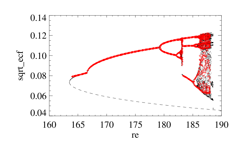
We next construct the low-dimensional system including as a parameter. Adding in the arguments of the system (equation (6)), the time increment maps are constructed for . In the construction of the low-dimensional system, 25 training points of , from to in increments of unity are used. For steady states in the range , we use one sample for each value of . For periodic states in the range , we use 50 sample points. Above the flow state may be turbulent and thus we use 100 sample points. Figure 6 shows the bifurcation structure of the constructed system by using these training points. Note that this diagram is shown by plotting eventual states, i.e. attractors, as a function of with increments being , which are much less than those in training points. It turns out that the constructed low-dimensional system well reproduces the bifurcation structure of the Navier–Stokes system even at many values of at which the training has not been done.
If a system can be constructed by a finite number of variables as mentioned above, any other quantities can also be represented by functions of these variables. Next, a physically important quantity is predicted as a function of a finite number of variables for the turbulent case using machine learning. We consider the total enstrophy as a function of , , , and energy input (), that is , which does not depend on time explicitly. All of these quantities are physically significant, and thus their functional relationship would provide us with implication of flow physics. Figure 7 shows the comparison of the construction of the function with the total enstrophy obtained from the DNS at . The function can be seen to predict the enstrophy for the Navier–Stokes system very precisely. In figure 8 the constructed function on the Poincaré section , , is shown. Colored points represent predicted on the attractor (see the color bar for the value of ), while gray objects are isosurfaces of and . Since the flow state is fully decided by these four quantities, and , the colored points are topological conjugate to the atractor. The constructed function can be seen to exhibit rather smooth and simple structure, and to monotonically depend on the energy input on the Poincaré section . We have confirmed that such properties are independent of the Poincaré section (different values of ). It is found that a dissipative state of intense highly localizes in phase space.


Using machine learning we have constructed low-dimensional map systems which predict precisely low-Reynolds-number turbulent flow in which the dimensions of attractors are very low. Once the system including the control parameter is constructed, trajectories of turbulence can be reproduced within much less CPU time than the DNS. The expression of a physically important quantity has also been obtained as a function of the variables in the constructed low-dimensional system, leading to deeper understanding of the relevance of phase space structure with flow physics. For a system in an extended domain or at high Reynolds number it is hard to construct the finite dimensional system directly from learning of the orbit , even if the dimension of attractors is much smaller than that treated in the DNS. Dimension reduction of feature quantity by deep learning may solve this problem in the near future.
This work was supported by JSPS KAKENHI and gAdvanced Computational Scientific Programh of Research Institute for Information Technology, Kyushu University. This work was performed on gPlasma Simulatorh (FUJITSU FX100) of NIFS with the support and under the auspices of the NIFS Collaboration Research program (NIFS16KNSS083).
[1]R. Temam, “Infinite-dimensional dynamical systems in mechanics and physics”,
Applied Mathematical Sciences Volume 68, 1988.
[2]T. Sauer, J.A. Yorke ans M. Casdagli, “Embedology” Journal of Statistical Physics, 65(3), 579-616, 1991.
[3]T. Kreilos and B. Eckhardt, “Periodic orbits near onset of chaos in plane Couette flow”,
Chaos, 22, 047505, 2012.
[4]A. Karatzoglou, A. Smola, K. Hornik and A. Zeileis “kernlab - An S4 Package for Kernel Methods
in R”, Journal of Statistical Software, 11(9), 1-10, 2004.
[5]I. Takeuchi, Q.V. Le, T.D. Sears and A.J. Smola, “Nonparametric Quantile Estimation”, Journal of Machine Learning Research, 7, 1231-1264, 2006.
[6]I. Shimada and T. Nagashima, “A Numerical Approach to Ergodic Problem of Dissipative Dynamical Systems”, Progress of Theoretical Physics, 61, 1605-1616, 1979.