Generalized Optimization of High Capacity Compressive Imaging Systems

MECA [11, 12] is an efficient extension to the physical optics (PO) method for penetrable and non-metallic objects. In MECA, scattering elements are discretized into triangular facets on which equivalent electric and magnetic currents are computed. By treating these currents as sources radiating in the background medium whose Green’s functions are known, MECA can compute the electric and magnetic fields at any position. Formally, the equivalent currents on the triangular facets are expressed as

where $\mathbf{\hat{n}}$ is the normal of the triangular surface, $\mathbf{H}_{t}$ and $\mathbf{E}_{t}$ are the total magnetic and electric fields, $\eta_{1}$ is the impedance of the background medium, $E_{TE_{i}}$ and $E_{TM_{i}}$ are the TE / TM components of the incident electric field, $\mathbf{\hat{e}}_{TE}$ is the unit vector for the TE component of the electric field, $\theta_{i}$ is the incident angle, and $\Gamma_{TE}$ and $\Gamma_{TM}$ are the TE / TM reflection coefficients. Assuming that the background medium is homogeneous, the scattered electric fields can be computed as follows:

where $k_{1}$ and $\lambda$ are the wavenumber and wavelength of the background medium, $\mathbf{r}$ is the point at which the scattered fields are evaluated, $\mathbf{\hat{r}}=\frac{\mathbf{r}}{\|\mathbf{r}\|_{\ell_{2}}}$, and $\mathbf{r}^{\prime}$ is a vector pointing from the center of the triangular surface to another point on the surface.

The terms in Eq. 10 - 12 can be separated into two groups: those that vary with the reflection coefficients, and those that do not. Taking this into consideration, we can express the discretized fields $\mathbf{g}_{t,i,m}\in\mathbb{C}^{N}$ radiated by the transmitting antenna as follows:

where $\mathbf{e}_{t,i,m}(\boldsymbol{x})\in\mathbb{C}^{N}$, $\mathbf{E}_{TE,t,i,m}(\boldsymbol{x})$ and $\mathbf{E}_{TM,t,i,m}(\boldsymbol{x})\in\mathbb{C}^{N\times L}$, $\mathbf{\Gamma}_{TE,t,m}(\boldsymbol{x})$ and $\mathbf{\Gamma}_{TM,t,m}(\boldsymbol{x})\in\mathbb{C}^{L}$, and $L$ is the number of triangular facets on the CRA. Similar expressions can be obtained for the receiving antennas, simply replace the $t$ subscript with $r$. In the most general scenario, $\mathbf{e}_{t,i,m}(\boldsymbol{x})$, $\mathbf{E}_{TE,t,i,m}(\boldsymbol{x})$, $\mathbf{E}_{TM,t,i,m}(\boldsymbol{x})$, $\mathbf{\Gamma}_{TE,t,m}(\boldsymbol{x})$, and $\mathbf{\Gamma}_{TM,t,m}(\boldsymbol{x})$ can all vary as a function of the design variables $\boldsymbol{x}$. Assuming that they are all differentiable, the partial derivatives $\frac{\partial\mathbf{g}_{t,i,m}(\boldsymbol{x})}{\partial x_{p}}$ can be expressed as follows:

Consider the scenario in which the design variables are the dielectric constant of purely dielectric scatterers. In this case, the fields $\mathbf{g}_{t,i,m}(\boldsymbol{x})$ and their derivatives can be expressed as follows:

Note that the Jacobian matrices $\frac{\partial\mathbf{\Gamma}_{TE,t,m}(\boldsymbol{x})}{\partial\boldsymbol{x}}$ and $\frac{\partial\mathbf{\Gamma}_{TM,t,m}(\boldsymbol{x})}{\partial\boldsymbol{x}}$ are diagonal because the number of reflection coefficients $L$ equals the number of design variables $P$. The reflection coefficients are computed by treating each facet of the CRA as a three-layer medium containing the background medium (i.e. freespace), the dielectric scatterer, and the perfect electric conductor (PEC) reflector. MECA considers the incident fields to be locally planar at each facet, such that the reflection coefficient of the $p-$th scatterer can be expressed as follows:

where $\Gamma_{bp,m}(\epsilon_{p})$ and $T_{bp,m}(\epsilon_{p})$ are the half-plane reflection and transmission coefficients going from the background medium to the dielectric, $\Gamma_{pb,m}(\epsilon_{p})$ and $T_{pb,m}(\epsilon_{p})$ are the half-plane reflection and transmission coefficients going from the dielectric to the background medium, $f_{m}$ is the frequency, $d_{p}$ is the thickness of the dielectric, and $\theta_{t_{t},m,p}(\epsilon_{p})$ is the angle of propagation in the dielectric. Note that we have replaced the generic design variable $x_{p}$ with the dielectric constant $\epsilon_{p}$ for clarity. Eq. 17 is a simplified version of the general relationship described in [16] for the case where the third medium is a PEC. It is straightforward to show that the derivatives of Eq. 17 and 18 can be expressed as follows:

To evaluate these equations, we require expressions for the transmission coefficients, reflection coefficients, and the propagation angle $\theta_{t_{t},m,p}(\epsilon_{p})$. The transmission and reflection coefficient formulations differ for the TE and TM modes, so we first consider the propagation angle. The following relationships for $\cos(\theta_{t_{t},m,p}(\epsilon_{p}))$ are easily found by invoking Snell’s Law:

where $\epsilon_{b}$ is the dielectric constant of the homogeneous background medium and $\theta_{i_{t},m,p}$ is the incident angle.

To simplify the notation when evaluating the transmission and reflection coefficients, we will drop the subscripts $m$ (measurement index), $t$ (transmitting antenna), and $p$ (dielectric scatterer index) on some of the parameters with the understanding that the formulations can be applied to all measurements and scatterers independently. According to electromagnetic theory, the half-plane TM reflection and transmission coefficients can be expressed as follows [17]:

It’s easy to show from Eq. 23 that the derivative $\frac{d\Gamma_{bp,TM}}{d\epsilon_{p}}$ can be expressed as follows:

Clearly, $\frac{dT_{bp,TM}}{d\epsilon_{p}}=\frac{d\Gamma_{bp,TM}}{d\epsilon_{p}}$, so it is omitted. The coefficients $\Gamma_{pb,TM}$ and $T_{pb,TM}$ and their derivatives can easily be found by exploiting the fact that $\Gamma_{pb,TM}=-\Gamma_{bp,TM}$, so they are also omitted.

The TE reflection and transmission coefficients can be expressed as follows [17]:

We first turn our attention to the reflection coefficient. The derivative $\frac{d\Gamma_{bp,TE}}{d\epsilon_{p}}$ can be expressed as follows:

Just as in the TM case, the reflection coefficient $\Gamma_{pb,TE}$ and its derivative can be obtained using the relationship $\Gamma_{pb,TE}=-\Gamma_{bp,TE}$.

We now turn our attention to the transmission coefficients. The derivative $\frac{dT_{bp,TE}}{d\epsilon_{p}}$ can be expressed as follows:

To compute $\frac{dT_{pb,TE}}{d\epsilon_{p}}$, we cannot simply replace the $\Gamma_{bp,TE}$ terms with $\Gamma_{pb,TE}$ due to the presence of the $\theta_{t}$ term in Eq. 26. This result is clear from Eq. 30:

It is now easy to show the following expression for $\frac{dT_{pb,TE}}{d\epsilon_{p}}$:

The dielectric CRA design method has been assessed using the test configuration displayed in Figure 1. In the design scenario, four receiving antennas (red dots) were used to measure the signals generated by the four transmitting antennas (green dots). The antennas operated in a multi-static configuration at ten frequencies uniformly spaced between $70.5$[GHz] and $77$[GHz], for a total of $160$ measurements. The antennas were modeled as horn antennas, wherein the incident electric field was oriented in the $+z$ direction and the direction of propagation was the $-x$ direction. The parabolic CRA reflector, which was located at $x=-0.5$[m], was discretized into $3750$ triangular facets. The design procedure was configured to optimize the dielectric constant of each triangular facet, wherein $\epsilon_{r}\in[1,30]$. All dielectrics had the same thickness $d=8.13$[mm], which is approximately two times the average wavelength of the operating frequencies. The imaging region consisted of $625$ positions uniformly spaced along a $0.2$[m] $\times$ $0.2$[m] grid centered at $x=0.9$[m]. The optimization problem of Eq. 5 was executed four times using the parameters listed in Table I. The first three configurations correspond to pure-capacity, pure-efficiency, and joint capacity and efficiency optimization of the sensing matrix, and the final configuration optimizes over all terms. To initialize the optimization procedure, the starting dielectric constant values were randomly selected over the feasible set.

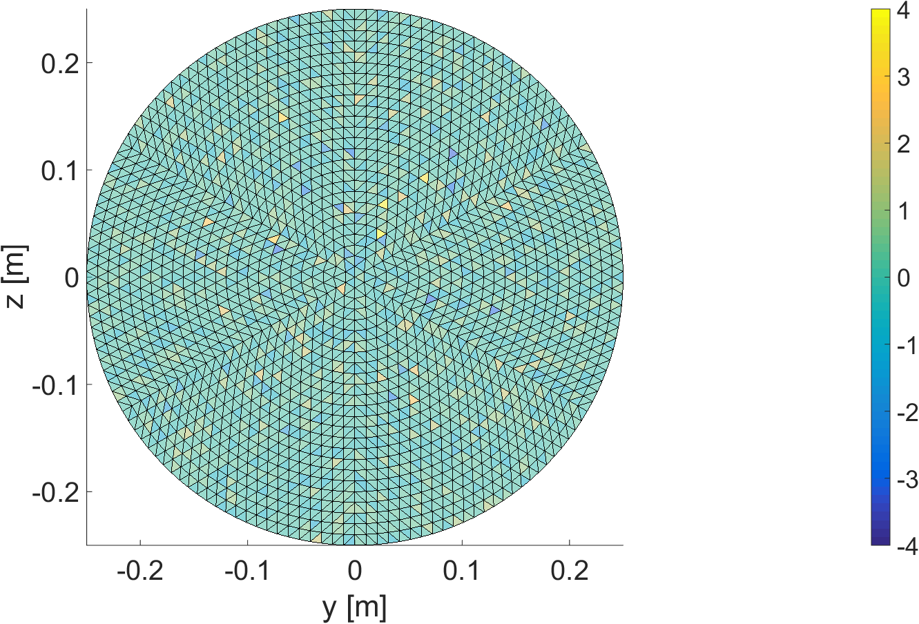
Figure 2 displays the dielectric constant of each triangular facet on the baseline randomized CRA, and Figures 3 - 6 display the difference in dielectric constant between the optimized CRA’s and the baseline randomized CRA. The change in dielectric constant varied for each of the design configurations, with the pure capacity optimization changing the least and the all terms configuration changing the most. Nevertheless, the design algorithm significantly improved the value of the objective function in each case. This can be seen in Tables II and III, which display the capacity and efficiency, respectively, of the sensing matrix and Green’s functions for the four design configurations and the baseline randomized CRA as a reference. A TRA is also included for reference. Each table element contains two values, the value of the metric (capacity or efficiency), and the difference between the achieved metric and the best metric achieved by any of the configurations. The optimal sensing matrix efficiency was achieved by optimizing only that metric. The optimal values for all other metrics were achieved by optimizing over all of the terms in Eq. 5.

Figure 7 displays the singular value distributions of the four optimized designs, the TRA, and the baseline randomized CRA. The TRA unsurprisingly has the worst sensing capacity of the six designs. The four optimized CRA’s have improved singular values compared to the randomized starting point, which in turn is an improvement over the TRA. The capacity-optimized and all terms optimized CRA’s have singular value distributions that are similar to the randomized CRA, except each singular value is approximately increased by a fixed amount. The efficiency-optimized CRA has the highest maximum singular value, but a less-uniform distribution than the capacity-optimized CRA. The joint capacity and efficiency-optimized CRA falls in between the others.

The singular value distributions suggest the following: $1)$ the CRA’s demonstrate better CS reconstruction capabilities than the TRA; $2)$ the randomized, capacity-optimized, and all terms optimized CRA’s demonstrate similar CS reconstruction capabilities in the absence of measurement noise; $3)$ the capacity-optimized and all terms optimized CRA’s demonstrate better CS reconstruction capabilities than the randomized CRA when the measurements are corrupted by noise due to their enhanced capacity. The first and second items are confirmed for this design scenario by Figure 8, which display the $\ell_{1}$-norm reconstruction capabilities of all antennas in the noiseless scenario. The third item is confirmed by Figure 9, which displays the $\ell_{1}$-norm reconstruction capabilities of all antennas in the presence of noise. Unsurprisingly, the efficiency-optimized and the joint capacity and efficiency-optimized CRA’s provide a CS reconstruction performance in between the randomized, capacity-optimized, and all terms optimized CRA’s.

The design method has also been assessed for a communication application in which there is a strong interfering signal located near $x=0.9$[m], $y=z=0$[m]. The objective, then, was to optimize the capacity of the receiver Green’s functions while simultaneously attenuating the interfering signal. This was achieved by solving Eq. 5 using the parameters displayed in Table IV. Figure 10 displays the difference in dielectric constant between baseline randomized CRA and the optimized CRA. Once again, the dielectric constants did not deviate significantly from the starting values. Nevertheless, the design algorithm produced a CRA that has an enhanced capacity ($-5747.1$ vs. $-5681.8$) and that significantly attenuates signals from the designated location. The latter property can be seen in Figures 11 and 12, which display the energy distribution of the Green’s functions for the baseline randomized CRA and the optimized CRA.

References

- [1] J. A. Martinez-Lorenzo, J. Heredia Juesas, and W. Blackwell, “A single-transceiver compressive reflector antenna for high-sensing-capacity imaging,” IEEE Antennas and Wireless Propagation Letters, 2015.
- [2] J. H. Juesas, G. Allan, A. Molaei, L. Tirado, W. Blackwell, and J. A. M. Lorenzo, “Consensus-based imaging using admm for a compressive reflector antenna,” in 2015 IEEE International Symposium on Antennas and Propagation USNC/URSI National Radio Science Meeting, July 2015, pp. 1304–1305.
- [3] R. Obermeier and J. A. Martinez-Lorenzo, “Model-based optimization of compressive antennas for high-sensing-capacity applications,” IEEE Antennas and Wireless Propagation Letters, 2016.
- [4] A. Busboom, H. D. Schotten, and H. Elders-Boll, “Coded aperture imaging with multiple measurements,” JOSA A, vol. 14, no. 5, pp. 1058–1065, 1997.
- [5] G. D. De Villiers, N. T. Gordon, D. A. Payne, I. K. Proudler, I. D. Skidmore, K. D. Ridley, C. R. Bennett, R. A. Wilson, and C. W. Slinger, “Sub-pixel super-resolution by decoding frames from a reconfigurable coded-aperture camera: theory and experimental verification,” in SPIE Optical Engineering+ Applications. International Society for Optics and Photonics, 2009, pp. 746 806–746 806.
- [6] R. F. Marcia and R. M. Willett, “Compressive coded aperture superresolution image reconstruction,” in Acoustics, Speech and Signal Processing, 2008. ICASSP 2008. IEEE International Conference on. IEEE, 2008, pp. 833–836.
- [7] E. J. Candès, J. Romberg, and T. Tao, “Robust uncertainty principles: Exact signal reconstruction from highly incomplete frequency information,” Information Theory, IEEE Transactions on, vol. 52, no. 2, pp. 489–509, 2006.
- [8] E. J. Candes, J. K. Romberg, and T. Tao, “Stable signal recovery from incomplete and inaccurate measurements,” Communications on pure and applied mathematics, vol. 59, no. 8, pp. 1207–1223, 2006.
- [9] D. L. Donoho, “Compressed sensing,” Information Theory, IEEE Transactions on, vol. 52, no. 4, pp. 1289–1306, 2006.
- [10] C. Rappaport, A. Morgenthaler, and M. Kilmer, “FDFD modeling of plane wave interactions with buried objects under rough surfaces,,” in 2001 IEEE Antenna and Propagation Society International Symposium, 2001, p. 318.
- [11] J. G. Meana, J. Á. Martinez-Lorenzo, F. Las-Heras, and C. Rappaport, “Wave scattering by dielectric and lossy materials using the modified equivalent current approximation (meca),” IEEE transactions on antennas and propagation, vol. 58, no. 11, pp. 3757–3761, 2010.
- [12] J. Gutiérrez Meana, J. Á. Martínez Lorenzo, and F. L. Las Heras Andrés, High frequency techniques: The physical optics approximation and the modified equivalent current approximation (MECA). InTech, 2011.
- [13] M. D. Migliore, “On electromagnetics and information theory,” Antennas and Propagation, IEEE Transactions on, vol. 56, no. 10, pp. 3188–3200, 2008.
- [14] M. D. Migliore and D. Pinchera, “Compressed sensing in electromagnetics: Theory, applications and perspectives,” in Antennas and Propagation (EUCAP), Proceedings of the 5th European Conference on. IEEE, 2011, pp. 1969–1973.
- [15] A. Beck and M. Teboulle, “A fast iterative shrinkage-thresholding algorithm for linear inverse problems,” SIAM Journal on Imaging Sciences, vol. 2, no. 1, pp. 183–202, 2009.
- [16] W. C. Chew, Waves and Fields in Inhomogeneous Media. IEEE Press, 1995.
- [17] F. T. Ulaby, E. Michielssen, and U. Ravaioli, “Fundamentals of applied electromagnetics 6e,” Boston, Massachussetts: Prentice Hall, 2010.