Configurational stability for the Kuramoto–Sakaguchi model

We consider the differential equation on $\mathbb{T}^{n}$:

where $i=1,\dots,n$, and the parameters $\omega_{i},\gamma\in\mathbb{R}$ and $\left|{\alpha}\right|<\pi/2$. This system was originally analyzed in a series of papers [13, 11, 12] and is commonly known today¹¹ 1 A rereading of the early literature suggests that a more fitting name for this system of equations would be the Sakaguchi–Shinomono–Kuramoto (SSK) system of equations, but against the weight of a consensus in the literature the gods themselves contend in vain. as the Kuramoto–Sakaguchi system [3, 10, 1, 5, 6]. This system is a generalization of the well-studied Kuramoto system, which is obtained by setting $\alpha$ to zero in (1.1). (In what follows, we will often refer to the system with $\alpha=0$ as the “standard Kuramoto” system.) The parameter $\alpha$ is alternatively called the phase-lag, detuning, or frustration parameter, see [8] for physical justification of each of these terms in the context of chemical oscillations.

This current work extends the spectral analysis performed upon the standard Kuramoto model originally pioneered in [9] and reconsidered in [2]. From a mathematical point of view, the addition of the nonzero $\alpha$ parameter leads to a significant increase in difficulty in the analysis of (1.1) as compared to standard Kuramoto. In [2], when $\alpha=0$, the system (1.1) is a gradient flow, and in particular the Jacobian at any fixed point is symmetric, simplifying the analysis considerably.

The addition of $\alpha$ also adds a level of dynamical complexity to this model. In standard Kuramoto, the center of mass of the system (1.1) rotates around the circle at a rate given by the average of the $\omega_{i}$; for fixed ${\boldsymbol{\omega}}$ any two solutions will precess at the same rate. In contrast, the system (1.1) can support multiple configurations that precess at different rates for the same ${\boldsymbol{\omega}}$. This is one feature that is in stark contrast to the standard Kuramoto model, and requires a rethinking of many of the intuitions associated with that model.

Generally we will find it useful to denote the vector field ${\mathbf{f}}\colon\mathbb{T}^{n}\rightarrow\mathbb{R}^{n}$ defined as

and we can write (1.1) compactly as

It is clear from this formulation that scaling $\gamma$ is equivalent to scaling ${\boldsymbol{\omega}}$, so in this paper we choose the convention throughout that $\gamma=1$.

We first note that our definition in (1.1) is slightly different than that commonly chosen in most studies, where there is no $\sin(\alpha)$ term. Of course, this only shifts the vector field by a constant amount and has no effect on the Jacobian of the system, but it has the nice normalization that ${\boldsymbol{\theta}}=0$ is a fixed point for ${\boldsymbol{\omega}}=0$ and any $\alpha$. In particular, notice that the function $\sin(\cdot-\alpha)+\sin\alpha$ has a fixed point at 0 with positive derivative whenever $\left|{\alpha}\right|<\pi/2$ — this makes it “most like” standard Kuramoto. In particular, it follows directly that if we choose ${\boldsymbol{\omega}}=0$ and any $\left|{\alpha}\right|<\pi/2$, then ${\boldsymbol{\theta}}=0$ is an attracting fixed point. Moreover, if we consider the family of functions $\sin(\cdot-\alpha)+\sin\alpha$ for $-\pi/2<\alpha<\pi/2$, then the effect is that the “stable” point at zero remains fixed, while one of the unstable points moves toward the origin, and at $\alpha=\pm\pi/2$ there is a saddle-node bifurcation.

The fundamental question considered in this paper is whether (1.1) (or (1.3)) admits a phase-locked solution and whether or not this solution is dynamically stable.

Note that ${\mathbf{f}}(\cdot,\alpha)$ has an $U(1)$ symmetry:

which necessitates the $\proj_{\mathbf{1}^{\perp}}$ in the definition above. Given any ${\boldsymbol{\theta}}_{0}\in\mathbb{R}^{n}$, we can choose ${\boldsymbol{\omega}}$ to make this a fixed point of our system, by choosing ${\boldsymbol{\omega}}_{0}=-{\mathbf{f}}({\boldsymbol{\theta}}_{0})$. Then ${\boldsymbol{\theta}}_{0}$ is a fixed point for (1.3) with ${\boldsymbol{\omega}}={\boldsymbol{\omega}}_{0}$. Let ${\boldsymbol{\theta}}(t)$ be a solution of (1.1) for some ${\boldsymbol{\omega}}_{0}$. Choose $\boldsymbol{\eta}(t)={\boldsymbol{\theta}}(t)+\kappa t{\bf 1}$.

where in the last line we exploited the $U(1)$ symmetry of ${\mathbf{f}}$. This means that shifting a solution with a constant velocity is equivalent to shifting the frequencies by a constant, and vice versa.

From this it follows that if ${\boldsymbol{\omega}}$ gives rise to a phase-locked solution, then ${\boldsymbol{\omega}}+c{\bf 1}$ does as well. Thus let us define:

For standard Kuramoto, the distinction between frequency slice and projection is not important as $L_{\omega}^{(0)}=P_{\omega}^{(0)}$. The fact that $L_{\boldsymbol{\omega}}^{(\alpha)}\neq P_{\boldsymbol{\omega}}^{(\alpha)}$ for general $\alpha$ might be surprising to those used to standard Kuramoto. For standard Kuramoto, fixed points, whether they be stable or unstable, always precess according to their average frequency. Additionally, for any ${\boldsymbol{\omega}}$ we can translate via $\boldsymbol{\eta}(t)$ with $\kappa=\frac{1}{n}\sum\omega_{i}$ to shift to an equivalent system with the new ${\boldsymbol{\omega}}$ lying in the mean zero plane $\mathbf{1}^{\perp}$. Then, for standard Kuramoto, $\mathbf{f}$ maps the mean zero plane in the configuration space ${\boldsymbol{\theta}}$ into the mean zero plane in the frequency space ${\boldsymbol{\omega}}$. However, this construction does not work for general $\alpha$.

We demonstrate this for $N=3$ oscillators in Figure 1 which depicts the sets $L_{\boldsymbol{\omega}}^{(\alpha)}$ and $R_{\boldsymbol{\omega}}^{(\alpha)}$ for $\alpha=0,\frac{\pi}{12},\frac{\pi}{6},\frac{\pi}{3}$. The coordinates are arranged as follows: the vector $\left(\frac{1}{\sqrt{3}},\frac{1}{\sqrt{3}},\frac{1}{\sqrt{3}}\right)^{t}$ is oriented in the $\hat{z}$ direction, while the graphs are drawn over the (mean zero) configuration space: ${\boldsymbol{\theta}}:=\hat{x}\left(\frac{1}{\sqrt{2}},-\frac{1}{\sqrt{2}},0\right)+\hat{y}\left(\frac{1}{\sqrt{6}},\frac{1}{\sqrt{6}},-\frac{2}{\sqrt{6}}\right)$. When $\alpha=0$ the set $L_{\boldsymbol{\omega}}^{(\alpha)}$ is two dimensional and agrees with the set $R_{\boldsymbol{\omega}}^{(\alpha)}$. (Note: for visual clarity the $R_{\boldsymbol{\omega}}^{(\alpha)}$ region has been shifted by one unit in the negative $\hat{z}$ direction. ) As $\alpha$ is increased $L_{\boldsymbol{\omega}}^{(\alpha)}$ becomes increasingly non-planar. Also note the loss of symmetry: when $\alpha=0$ the region has symmetry group $D_{6}$, but for $\alpha\neq 0$ the symmetry group is $D_{3}.$ When $\alpha=0$ the standard Kuramoto is invariant under permutations of the oscillators along with ${\boldsymbol{\theta}}\mapsto-{\boldsymbol{\theta}},{\boldsymbol{\omega}}\mapsto-{\boldsymbol{\omega}}$. This symmetry is lost for non-zero $\alpha$.

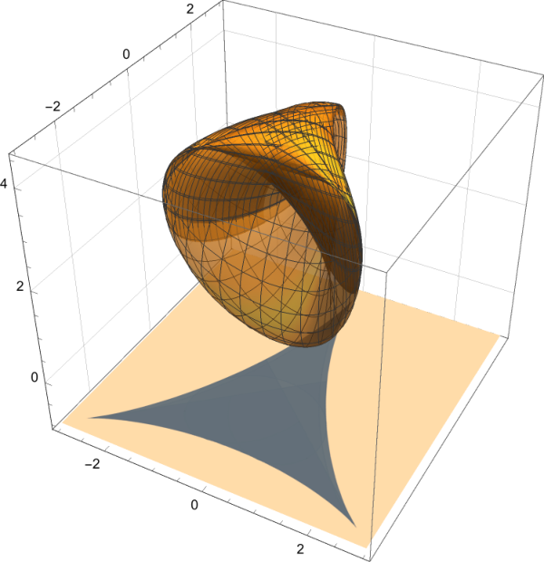
The lifting of $L_{\boldsymbol{\omega}}^{(\alpha)}$ out of the mean zero plane has a very interesting impact on solutions. For $\alpha\neq 0$, there are choices of pairs ${\boldsymbol{\theta}},{\boldsymbol{\omega}}$ such that ${\boldsymbol{\theta}}$ is a fixed point (and thus has average velocity zero) while the ${\boldsymbol{\omega}}$ has nonzero average! Again using an specific $\boldsymbol{\eta}$–shift, we can also see that this implies that there are cases with $\sum\omega_{i}=0$, but (1.1) supports precessing phase-locked solutions. Continuing in this direction, the system (1.1) can support solutions that precess at different velocities for even the same ${\boldsymbol{\omega}}$. We exhibit this in the case $n=3$. Modding for translations and reflections, for standard Kuramoto there are six fixed points (with zero angular velocity):

(Note: for clarity, we have not projected these fixed-points into the mean zero plane.) For Kuramoto–Sakaguchi with ${\boldsymbol{\omega}}\neq 0$, there are still six phase-locked solutions. However these different phase-locked solutions rotate with different angular frequencies. To see this, first note that ${\mathbf{f}}((0,0,0),\alpha)=(0,0,0)$, so the solution with all angles the same is a fixed point for ${\boldsymbol{\omega}}=0$. If we next consider the twist state $(0,2\pi/3,4\pi/3)$, we can compute ${\mathbf{f}}((0,2\pi/3,4\pi/3),\alpha)=3\sin\alpha(1,1,1)$. Thus this solution rotates with angular velocity $3\sin\alpha$ or (equivalently) is a fixed point for ${\boldsymbol{\omega}}=-3\sin\alpha(1,1,1)$. Thus we see that ${\boldsymbol{\omega}}=0$ supports both the fixed point ${\boldsymbol{\theta}}=0$ and the phase-locked equilateral configuration which rotates at velocity $3\sin\alpha$.

For the three fixed points that are permutations of a single $\pi$, the situation is slightly more complicated, in that the equilibrium configuration depends on the parameter $\alpha$. For example, to consider solutions near to $(0,\pi,0)$, we write ${\boldsymbol{\theta}}(\alpha)=(0,\pi+\varphi(\alpha),0)$. Then we see that

If these components are all equal, we obtain a phase-locked solution. This condition is the functional equation

which is equivalent to

Applying some trigonometric identities this can be solved to find that

As before, $(0,\pi+\varphi(\alpha),0)$ is a fixed point for the system with ${\boldsymbol{\omega}}=-(\sin(\alpha)+\sin(\alpha-\varphi(\alpha)))(1,1,1)$. Equivalently, we see that ${\boldsymbol{\omega}}=0$ support the solution ${\boldsymbol{\theta}}(t)=(0,\pi+\varphi(\alpha),0)-(\sin(\alpha-\varphi(\alpha))+\sin(\alpha))(1,1,1)$, which rotates at velocity $\sin(\alpha)+\sin(\alpha-\varphi(\alpha))$.

In the spirit of the work in [2], we begin by recasting the Jacobian of the forcing function of (1.1) as a low-rank perturbation of a diagonal matrix.

The fact that the Jacobian matrix of the flow can be written as the sum of a diagonal piece and a low-rank (rank two) piece will simplify the spectral analysis.

Additionally, examining the original statement of ${\bf J}$ (1.3) we can easily see that for any $\boldsymbol{\theta}$ all the row sums of the matrix ${\bf J}$ are always zero. This leads to our second observation.

The function $\mathbf{f}:\mathbb{T}^{n}\rightarrow\mathbb{R}^{n}$ is a natural map from the configuration space $\mathbb{T}^{n}$ to the frequency space $\mathbb{R}^{n}$. Since (1.1) is invariant under the one-parameter family of rotations $\theta_{i}\rightarrow\theta_{i}+s$, we can restrict our work in $\mathbb{T}^{n}$ to the mean-zero plane, $\sum\theta_{i}=0$. In other words, we need only consider $\boldsymbol{\theta}$ an element of the reduced configuration space $\mathcal{T}:=\mathbb{T}^{n}\bigcap\mathbf{1}^{\perp}$.

As demonstrated in Figure 1, the range of the map $\mathbf{f}$ is not all of $\mathbb{R}^{n}$. However, provided we can show that the set $\mathcal{S}_{\theta}$ is non-empty, then the image of the reduced configuration space will be an $n-1$ dimensional surface in $\mathbb{R}^{n}$. It is clear that $\mathcal{S}_{\omega}$ is the important object for studying synchronization: All questions about the probability of full synchrony are questions about the size of $\mathcal{S}_{\omega}$ in some measure. One of the key ingredients in this is a good characterization of $\mathcal{S}_{\omega}$. In standard Kuramoto, it is common at this point to reduce the frequency space of $\boldsymbol{\omega}$ to the mean-zero plane as well, but this is not possible as discussed above. Nonetheless, $\mathbf{f}$ remains a well-defined map for the Kuramoto-Sakaguchi model between $\mathcal{S}_{\theta}$ and $\mathcal{S}_{\omega}$. Colloquially, $\mathcal{S}_{\omega}$ can be thought of as a graph over $\mathcal{S}_{\theta}$ and in the orientation of Figure 1 we will see that $\mathcal{S}_{\omega}$ is the bottom surface of the object.

Finally, note that $f(\mathbf{0})=\mathbf{0}$, the derivative of $\mathbf{f}$ is the Jacobian $\mathbf{J}$, and the dimension of the kernel of $\mathbf{J}$ is one at the origin, so at least in a neighborhood of the origin, $S_{\omega}$ is a manifold of the same dimension as $S_{\theta}$.

For any $|\alpha|<\pi/2$, there is a neighborhood of $\mathbf{0}$ such that all the diagonal entries $D_{ii}$ are negative. Since $\mathbf{J}$ is not symmetric, as $s$ increases from zero to one in (2.1), the eigenvalues need not be monotone increasing. However, for a particular subset of $\mathcal{T}$, we can control the top eigenvalue. If we can then show that the top eigenvalue is 0, then we will necessarily have a $\theta$ that must be in the set of $\mathcal{S}_{\theta}$. To do so, we need a couple of corollaries to the Perron–Frobenius Theorem [7, Section 8.4]. For completeness, we will state the relevant portion of the theorem:

Although Perron–Frobenius is typically stated for a matrix with all positive entries, the really important mechanism is the positivity of the off-diagonal entries. Specifically, we have:

In order to use these results on ${\bf J}(s)$, we will need to be slightly more careful about the region in $\mathcal{T}$ that we use. Recall that ${\bf A}=[\cos(\theta_{j}-\theta_{i}-\alpha)]$ (1.7). To use the corollary, we need to restrict $\boldsymbol{\theta}$ further.

Note that for any element of $\mathcal{S_{\theta}^{{\dagger}}}$, the diagonal of ${\bf D}$ will have all negative entries.

We recognize that $\mathcal{S_{\theta}^{{\dagger}}}$ is not necessarily a complete description of $\mathcal{S_{\theta}}$. In fact, there are likely stationary solutions in $\mathcal{T}$ that are not stable, and thus not in $\mathcal{S_{\theta}}$. To further understanding the stability properties of the stationary solutions, we return to the one-parameter family of matrices ${\bf J}(s)={\bf D}+s{\bf A}$ and we define the following index.

Our goal is to detect eigenvalue crossings into the right-half plane as $s$ increases from 0 to 1. A reasonably straightforward linear algebra calculation gives a nice representation of the characteristic polynomial of ${\bf J}(s)$.

While the non-self-adjoint nature of the operator makes it difficult to get results as sharp as those in the standard Kurammoto model, we can establish a sufficient condition for instability. The main observation here is that, since ${\bf J}(s)$ is real the eigenvalues occur in complex conjugate pairs, and thus the index $n_{+}({\bf J}(s))$ can change in the following ways

• •

  $n_{+}({\bf J}(s))$ can change by one when a real eigenvalue passes through the origin.

• •

  $n_{+}({\bf J}(s))$ can change by two when a complex conjugate pair of eigenvalues crosses the imaginary axis.

The first of these possibilities is easy to detect, as it is signalled by the vanishing of $P_{{\bf J}}(s)$. The second is not so easy to detect, thus motivating us to count modulo two.

We begin with a visualization of the three oscillator model, $N=3$. For any $\alpha$, the map $\mathbf{f}$ is rotationally invariant in the configuration space $\boldsymbol{\theta}$. Thus the image of the reduced configuration space $\mathcal{T}:=\mathbb{T}^{3}\bigcap\mathbf{1}^{\perp}$ under the map $\mathbf{f}$ will be a 2-dimensional surface in the 3-dimensional $\boldsymbol{\omega}$-space. Figure 2 is the surface $\mathbf{f}(\mathcal{T})$ associated with the fixed detuning parameter $\alpha=\pi/6$.

We are interested in the portion of this surface that corresponds to $\mathcal{S}_{\omega}:=\mathbf{f}(\mathcal{S}_{\theta})$, the ${\boldsymbol{\omega}}$ that give rise to a phase-locked solutions. To see this, we return to the pre-image $\mathcal{T}$. Again the $\mathbf{1}^{\perp}$ plane is spanned by $\mathbf{e}_{1}=(1,-1,0)/\sqrt{2}$ and $\mathbf{e}_{2}=(1,1,-2)/\sqrt{6}$. In the local coordinates defined by $\mathbf{e}_{1}$ and $\mathbf{e}_{2}$, the phase diagram for three oscillators (where $\alpha=\pi/6$) is summarized in Figure 3.

In this image, $\mathcal{S}_{\theta}$ and $\mathcal{S}_{\omega}$ are paired side-by-side. The blue regions corresponds to the stable region in local coordinates, where the Jacobian of $\mathbf{f}$ is negative semi-definite with a one dimensional kernel. The gold and red regions correspond to when the Jacobian of $\mathbf{f}$ has one or two unstable eigen-direction, respectively. For added clarity, we have the frequency space de-constructed by index in Figure 4. We note that stable set here corresponds exactly to the bottom of the $\alpha=\pi/6$ surface in the orientation of Figure 1 (when we discussed the frequency region $R_{\boldsymbol{\omega}}^{(\alpha)}$ in Section 1.2).

Determining the probability for a Kuramoto system to admit a phased locked solution when ${\boldsymbol{\omega}}$ is randomly assigned is directly related to understanding the size of the frequency space $\mathcal{S}_{\omega}$. For standard Kuramoto, $\mathcal{S}_{\theta}$ is a convex set that is invariant under the actions of the dihedral group of order $N$ (see [2]). Moreover, these geometric properties are preserved under the map $\mathbf{f}$ when $\alpha$ is zero. This is due to the fact that when $\alpha=0$, $\mathbf{f}$ is an odd function and the reflections ${\boldsymbol{\omega}}\rightarrow-{\boldsymbol{\omega}}$ and ${\boldsymbol{\theta}}\rightarrow-{\boldsymbol{\theta}}$ admit another stable solution. In the end, excellent estimates exist for the size of $\mathcal{S}_{\omega}$ for the standard model. This geometry does not hold for the Kuramoto-Sakaguchi model. In Figure 5, we have the boundary of $\mathcal{S}_{\theta}$ for values of $\alpha$ ranging from zero to $5\pi/12$. The “hexagonal” red curve corresponds to standard Kuramoto. All other boundary curves loose the extra geometric structure and possess only triangular symmetry. In fact, it is easy to see the same behavior in the $N=4$ model. In Figure 7, the corresponding pictures are all in local coordinates as we are unable to embed $\mathcal{S}_{\omega}$ in its natural space. None the less, the symmetry and reduction of dihedral order is easily prevalent. In keeping with earlier conventions, the blue regions in Figure 6 correspond to the stable region $\mathcal{S}_{\theta}$ in local coordinates for varying $\alpha$. We know that standard Kuramoto possesses octahedral symmetry, while we can see that all other configuration spaces correspond to tetrahedral symmetry. Moreover, in Figure 7 this symmetry is preserved (in local coordinates) under the mapping $\mathbf{f}$.

As $\mathcal{S}_{\omega}$ no longer resides in the $\mathbf{1}^{\perp}$ plane, we can’t use convexity to estimate its size. But at the outset of our study, there was no reason to believe $\mathcal{S}_{\theta}$ would not be so and we hoped to use the size of $\mathcal{S}_{\theta}$ to estimate the size of the stable region. For large $\alpha$, the convexity of $\mathcal{S}_{\theta}$ is lost. In Figure 5, the fuchsia colored boundary curve corresponds to $\alpha=7\pi/24$ and the associated $\mathcal{S}_{\omega}$ is clearly no longer convex. The same loss of convexity can be seen in the four oscillator model. In Figure 6,the configuration space corresponding to $\alpha=2\pi/7$ is not convex. In the end we were unable to develop a geometric approach to estimating the size of the stable region. In Section 3.3, we appeal to a purely numeric approach to estimate the size.

References

- [1] D. Amadori, S. Y Ha, and J. Park. On the global well-posedness of BV weak solutions to the Kuramoto-Sakaguchi equation. J. Diff. Eq., 262(2):978–1022, 2017.
- [2] J. C. Bronski, L. DeVille, and M. J. Park. Fully synchronous solutions and the synchronization phase transition for the finite- Kuramoto model. Chaos, 22(3):033133, 17, 2012.
- [3] F. De Smet and D. Aeyels. Partial entrainment in the finite Kuramoto-Sakaguchi model. Phys. D, 234(2):81–89, 2007.
- [4] T. Ferguson. Dynamical Systems on Networks. PhD thesis, University of Illinois, 2018.
- [5] Seung-Yeal Ha, Hwa Kil Kim, and Jinyeong Park. Remarks on the complete synchronization for the Kuramoto model with frustrations. Analysis and Applications, pages 1–39, 2017.
- [6] Seung-Yeal Ha, Dongnam Ko, and Yinglong Zhang. Emergence of phase-locking in the Kuramoto model for identical oscillators with frustration. SIAM Journal on Applied Dynamical Systems, 17(1):581–625, 2018.
- [7] Roger A. Horn and Charles R. Johnson. Matrix analysis. Cambridge University Press, Cambridge, second edition, 2013.
- [8] I.Z. Kiss, Y. Zhai, and J.L. Hudson. Predicting mutual entrainment of oscillators with experiment-based phase models. Phys. Rev. Lett., 94:248301, 2005.
- [9] R. E. Mirollo and S. H. Strogatz. The spectrum of the locked state for the Kuramoto model of coupled oscillators. Phys. D, 205(1-4):249–266, 2005.
- [10] E Omel?chenko and Matthias Wolfrum. Bifurcations in the Sakaguchi–Kuramoto model. Physica D: Nonlinear Phenomena, 263:74–85, 2013.
- [11] H. Sakaguchi, S. Shinomoto, and Y. Kuramoto. Local and global self-entrainments in oscillator lattices. Prog. Theor. Phys., 77(5):1005–1010, 1987.
- [12] H. Sakaguchi, S. Shinomoto, and Y. Kuramoto. Mutual entrainment in oscillator lattices with nonvariational type interaction. Prog. Theor. Phys., 79(5):1069–1079, 1988.
- [13] Shigeru Shinomoto and Yoshiki Kuramoto. Phase transitions in active rotator systems. Progress of Theoretical Physics, 75(5):1105–1110, 1986.