Cross-Layer Energy Efficient Resource Allocation in PD-NOMA based H-CRANs: Implementation via GPU

In next cellular communication systems, power domain - non-orthogonal multiple access (PD-NOMA) is a novel multiple access scheme which is a promising candidate for the fifth generation (5G) cellular communication systems [1]. PD-NOMA multiplexes different users symbols by applying the superposition coding (SC) technique at the transmitter side, while at the receiver side the successive interference cancellation (SIC) technique is applied to recover back the multiplexed symbols [1].

Heterogeneous cloud radio access network (H-CRAN) is a novel architecture which is proposed as a promising technology for next cellular communication systems [2]. H-CRAN combines heterogeneous cellular network (HCN) with cloud radio access network (C-RAN). In addition, H-CRAN covers the advantages of C-RAN and HCN at the same time [2]. The main subsystems of the H-CRAN architecture are the baseband unit (BBU) pool, fiber links and remote radio heads (RRHs) where one of the RRHs is a high power node (HPN) and the others are low power nodes (LPNs). Instead of the processing that is distributed at the base stations (BSs) in the HCN, a centralized signal processing is applied in the BBU pool which reduces the manufacturing and operating cost. Moreover, a cooperation between different RRHs is permitted due to the centralized signal processing, thus spectrum efficiency and link reliability are improved. The RRHs compress and forward the received signals from the user to the BBU pool via high bandwidth and low latency fiber links [2]. Therefore, H-CRANs improve the users quality of service (QoS), the spectral efficiency (SE) of the system and increase the network architecture flexibility. Moreover, H-CRANs decrease the power consumption of the system, and PD-NOMA technique improves the system throughput, SE, and energy efficiency (EE) of the fifth generation (5G) cellular communication systems. In order to cover the advantages of H-CRAN and PD-NOMA technique at the same time, we consider PD-NOMA based H-CRAN system.

Due to the enormous increase in mobile data traffic and the complexity of the proposed technologies including PD-NOMA and H-CRAN, a high computational processing is needed where the conventional methods can not tackle this issue. Therefore, we seek toward a new processing method which accelerates the processing time. Graphics Processing Unit (GPU), due to the advantage of its massive number of cores and its parallelism directives, handles the works with parallel data [3, 4, 5, 6, 7]. Accelerating applications and simulations with using GPUs has turned out to be progressively well-known from 2006 [8]. OpenACC is an open GPU directives standard which makes GPU programming simple and portable over the parallel multi-core processors [3]. In [9], a communication optimization for multi GPU implementation of Smith-Waterman Algorithm is investigated. In [6], stochastic finite-difference time domain method is investigated on GPU by employing OpenACC application program interface (API).

During the past decade, numerous energy efficient (EE), BS selection and cross layer resource allocation problems for OFDMA systems are investigated [2, 10, 11, 12, 13, 14, 15]. Furthermore, different PD-NOMA systems are studied [16, 17, 18, 19, 20].

In [10], the EE orthogonal frequency division multiplexing (OFDM) relay system is developed where both the transmit and circuit power consumptions are considered. The EE power allocation for OFDM based cognitive radio networks is investigated in [11]. BS or cell selection for the mobile user is investigated in [13, 14]. In [15], a cross layer resource allocation scheme for OFDMA systems is investigated. In [2], the EE resource allocation in H-CRANs is studied, where RRHs are basically utilized to supply high data rates for users with high quality of service (QoS) requirements, while HPN is created to ensure the coverage and serve users with low QoS requirements. In [2], the number of RRHs is supposed to be sufficiently large, then the considered overall EE optimization problem of the H-CRAN system is approximated to EE optimization problem for only one RRH.

In [21], a comprehensive overview of the latest NOMA research and innovations as well as their applications are summarized and discussed. In [16], the effect of user pairing on the performance of PD-NOMA systems is investigated. A power allocation in OFDM-NOMA system is studied in [17], where a single BS is taken into consideration. In [18], joint power and channel allocation for PD-NOMA in 5G downlink cellular systems by considering one BS is developed. In [19, 20], the radio resource allocation for HCNs based on PD-NOMA is studied. In [22], robust radio resource allocation for a cellular system based on PD-NOMA is investigated.

To the best of our knowledge, cross layer resource allocation and RRH selection problems neither for systems based on PD-NOMA technique nor for H-CRAN have been investigated yet. As well, resource allocation for H-CRAN systems neither based on PD-NOMA nor with heterogeneous traffic have been studied so far. Moreover, successive convex approximation for low complexity (SCALE) [23] with the Lagrangian method has not been analyzed on GPU using OpenACC API yet.

In our work, we consider a cross layer EE radio resource allocation and RRH selection problem for heterogeneous traffic in PD-NOMA based H-CRANs. In this formulation, two types of traffic are taken into account, elastic traffic and streaming traffic. In our design, first, the radio resources are assigned to the streaming traffic users in a way that the streaming users QoS constraints are satisfied. Thereafter, the remaining radio resources are assigned to the elastic traffic users. The optimization problem is to maximize the energy efficiency of the elastic users where the total power consumption is partitioned to three parts: 1) the power consumption in the fiber links depending on the active RRHs, 2) the power consumption of RRHs and 3) the circuit power consumption [2]. Moreover, due to utilizing the PD-NOMA technique more than one user can be allocated at the same subcarrier and each user can be served by only one RRH. The considered EE optimization problem is non-convex, intractable, and NP-hard. Therefore, we solve the considered optimization problem by applying the successive convex approximation (SCA) method. Therefore, in our paper, we focus on both resource allocation and remote radio head selection. Then, due to the different factors taken into account which are from power allocation, subcarrier allocation and remote radio head selection, and at the same time the enormous increase in mobile data traffic, a high computational processing is needed where the conventional methods can not tackle this issue. Moreover, increasing the number of variables in the system which means increasing the number of parameters is beneficial since it makes the system more flexible in allocating the energy efficiency which helps in maximizing the energy efficiency of the system. Thus, to accelerate the processing speed, we introduce a framework for SCALE with the Lagrangian method on GPU and we run the proposed optimization problem on GPU by utilizing OpenACC API. Moreover, in order to evaluate the optimality gap of the proposed solution, we solve the considered optimization problem by applying an optimal algorithm based on the monotonic optimization [24, 25, 26]. Simulation results confirm that the energy efficiency performance of the H-CRAN based on the PD-NOMA method is approximately 14% more than the systems based on orthogonal multiple access (OMA) where only one user can be selected on each subcarrier. Moreover, simulation results show that the system energy efficiency in H-CRAN scenario is enhanced compared to the conventional, C-RAN, HCN and 1-tier HPN scenarios.

The key contributions of this paper are summarized as follows:

• •

  We propose a cross layer EE radio resource allocation and RRH selection algorithm for heterogeneous traffic in PD-NOMA based H-CRANs.

• •

  We prove the convergence of the SCA approach for the cross layer EE radio resource allocation and RRH selection in PD-NOMA based H-CRANs and we highlight on the performance improvements of the NOMA technique.

• •

  We solve the considered optimization problem by applying the monotonic optimization method. First, we transform the optimization problem to a monotonic one in a canonical form, then we obtain the solution by applying the polyblock algorithm.

• •

  We introduce a framework for accelerating SCALE with the Lagrangian method on GPU and we run the proposed optimization problem by using OpenACC API on GPU.

The reminder of this paper is organized as follows. In Section II, we describe the system model and problem formulation of our design. The transformation of the fractional objective function problem to a problem with an objective function with subtractive form is introduced in Section III. The proposed approaches to solve the equivalent cross layer EE resource allocation and RRH selection problem are presented in Section IV. Computational complexity of the proposed solution methods are studied in Section V. Distributed solution and signalling overhead of both the centralized and distributed solutions are investigated in Section VI. A framework for accelerating the general SCALE with the Lagrangian method using GPU is proposed in Section VII. The performance of the proposed algorithm and our system model through different numerical experiments are examined in Section VIII. Lastly, we conclude the paper in Section IX.

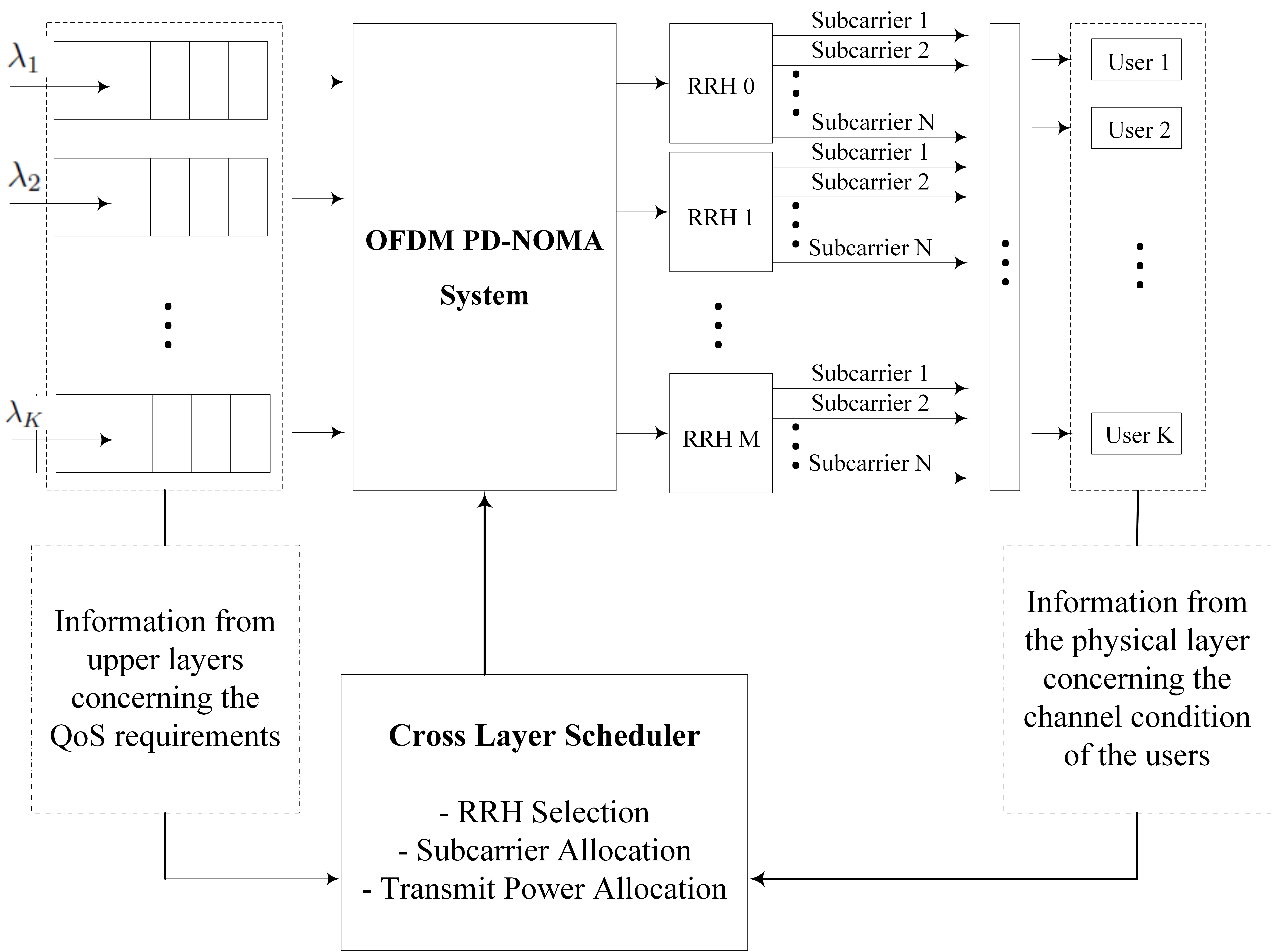
We consider a two tier downlink H-CRAN, where a typical illustration example of this network is presented in Fig. 1. As well, the proposed cross layer with RRH selection system in PD-NOMA H-CRANs is shown in Fig. 2. In this network, $M_{f}$ LPN RRHs and one HPN RRH cover the desired coverage area sharing the available radio spectrum. Table I summarizes the parameters and symbols used in the system model and problem formulation.

The RRHs set is denoted by $\mathcal{M}=\{0,1,2,...,M_{f}\}$, where $0$ is the index of the HPN RRH and $\mathcal{M}_{f}=\{1,2,...,M_{f}\}$ is the set of the LPN RRHs. $M=M_{f}+1$ is the number of all RRHs. We denote the set of all users by $\mathcal{K}=\{1,2,...,K\}$. The users set is split into two sets: 1) streaming users set $\mathcal{K}^{s}=\{1,2,...,K^{s}\}$ and 2) elastic users set $\mathcal{K}^{e}=\{1,2,...,K^{e}\}$. The number of streaming users and elastic users are equal to $K^{s}=|\mathcal{K}^{s}|$ and $K^{e}=|\mathcal{K}^{e}|$, respectively. Therefore, $\mathcal{K}=\mathcal{K}^{e}\cup\mathcal{K}^{s}$ and the number of all users is $K=K^{s}+K^{e}$. Due to the PD-NOMA technique, over each subcarrier in RRH $m$, $l$ users can be allocated where $l\leq K$.

In this system model, we suppose the system bandwidth is equal to $B$ partitioned to $N$ subcarriers with bandwidth $B_{n}=B/N$ and the subcarriers set is denoted by $\mathcal{N}=\{1,2,...,N\}$. $h_{m,k}^{(n)}$ denotes the channel gain from RRH $m$ to user $k$ over subcarrier $n$ and $\Gamma_{m,k}^{(n)}=|h_{m,k}^{(n)}|^{2}$. Due to using the PD-NOMA technique, signals of users with better channel condition is considered as noise while the signals of users with weaker channel condition can be successfully decoded and removed during the decoding process [27, 28, 29]. Then, the RRH $m$ transmits $\sum_{k\in\mathcal{K}}A_{m,k}^{(n)}\rho_{m,k}^{(n)}\sqrt{p_{m,k}^{(n)}}s_{m,k}^{(n)}$ over subcarrier $n$ where $s_{m,k}^{(n)}$ is the information signal for the $k^{th}$ user from RRH $m$ over subcarrier $n$, $p_{m,k}^{(n)}$ represents the transmit power from RRH $m$ to user $k$ over subcarrier $n$ and $\rho_{m,k}^{(n)}$ is a binary variable as user and subcarrier allocation indicator where $\rho_{m,k}^{(n)}=1$ if user $k$ is allocated over the subcarrier $n$ in RRH $m$ and equal to zero otherwise.

As well, $A_{m,k}$ is a binary variable as user and RRH allocation indicator where $A_{m,k}=1$ if user $k$ is served by RRH $m$ and equal to zero otherwise. Then we denote $\boldsymbol{\rho}_{m,k}=[\rho_{m,k}^{(1)},\rho_{m,k}^{(2)},...,\rho_{m,k}^{(N)}]$, $\boldsymbol{\rho}_{m}=[\boldsymbol{\rho}_{m,1},\boldsymbol{\rho}_{m,2},...,\boldsymbol{\rho}_{m,K}]$ and $\boldsymbol{\rho}=[\boldsymbol{\rho}_{0},\boldsymbol{\rho}_{1},...,\boldsymbol{\rho}_{M_{f}}]$. Moreover, we denote $\textbf{p}_{m}^{(n)}=[p_{m,0}^{(n)},p_{m,1}^{(n)},...,p_{m,K}^{(n)}]$, $\textbf{p}^{(n)}=[\textbf{p}_{0}^{(n)},\textbf{p}_{1}^{(n)},...,\textbf{p}_{M_{f}}^{(n)}]$, $\textbf{p}_{m,k}=[p_{m,k}^{(1)},p_{m,k}^{(2)},...,p_{m,k}^{(N)}]$, $\textbf{p}_{m}=[\textbf{p}_{m,1},\textbf{p}_{m,2},...,\textbf{p}_{m,K}]$ and $\textbf{p}=[\textbf{p}_{0},\textbf{p}_{1},...,\textbf{p}_{M_{f}}]$.

As such, the signal to interference plus noise ratio (SINR) of user $k$ over subcarrier $n$ in RRH $m$ after performing SIC is $\gamma_{m,k}^{(n)}=\frac{p_{m,k}^{(n)}\Gamma_{m,k}^{(n)}}{\sigma_{m,k}^{(n)}+I_{m,k}^{(n)}}$ where $\sigma_{m,k}^{(n)}$ is the noise power at user $k$ in RRH $m$ over subcarrier $n$ and $I_{m,k}^{(n)}=\sum_{i\in\mathcal{K},\Gamma_{m,k}^{(n)}\leq\Gamma_{m,i}^{(n)},i\neq k}A_{m,i}^{(n)}\rho_{m,i}^{(n)}p_{m,i}^{(n)}\Gamma_{m,k}^{(n)}+\sum_{j\in\mathcal{M}/{\{m\}}}\sum_{i\in\mathcal{K}}A_{j,i}^{(n)}\rho_{j,i}^{(n)}p_{j,i}^{(n)}\Gamma_{j,k}^{(n)}$ is the received interference power from the multiplexed users at the same subcarrier and other RRHs.

Based on information theory, in a PD-NOMA based system, user $k$ can successfully detect the signals of user $k^{\prime}$ which has less SINR than that of user $k$, if the SINR of user $k^{\prime}$ at user $k$ is higher than its own SINR [16, 30]. Therefore, mathematically we have $\gamma_{m,k}^{(n)}(k^{\prime})\geq\gamma_{m,k^{\prime}}^{(n)}(k^{\prime})$, where $\gamma_{m,k}^{(n)}(k^{\prime})$ is the SINR of user $k^{\prime}$ at user $k$ and $\gamma_{m,k^{\prime}}^{(n)}(k^{\prime})$ is the SINR of user $k^{\prime}$. Consequently, from the SINR definition, we have $\frac{p_{m,k^{\prime}}^{(n)}\Gamma_{m,k}^{(n)}}{\sigma_{m,k}^{(n)}+I_{m,k}^{(n)}}\geq\frac{p_{m,k^{\prime}}^{(n)}\Gamma_{m,k^{\prime}}^{(n)}}{\sigma_{m,k^{\prime}}^{(n)}+I_{m,k^{\prime}}^{(n)}}$, where it is equivalent to

The rate of user $k$ over subcarrier $n$ in RRH $m$ is adopted by $r_{m,k}^{(n)}(\textbf{p}^{(n)})=\log_{2}(1+\gamma_{m,k}^{(n)}(\textbf{p}^{(n)}))$. Then, the full achievable rate of the user $k$ is expressed as $r_{k}(\textbf{A},\boldsymbol{\rho},\textbf{p})=\sum_{m\in\mathcal{M}}A_{m,k}w_{m,k}\sum_{n\in\mathcal{N}}\rho_{m,k}^{(n)}r_{m,k}^{(n)}(\textbf{p}^{(n)})$, where $w_{m,k}\in[0,1]$ is a priority weight of the user $k$ in RRH $m$. By regulating these weights, the behavior of proportional fairness between users can be enforced and a trade-off between the user’s rate can be adopted and different QoSs or importance levels can be placed by the operator [31, 32, 33]. Therefore, the total weighted sum rate of the elastic users can be calculated by $R({\textbf{A},\boldsymbol{\rho},\textbf{p}})=\sum_{m\in\mathcal{M}}\sum_{k\in\mathcal{K}^{e}}A_{m,k}w_{m,k}\sum_{n\in\mathcal{N}}\rho_{m,k}^{(n)}r_{m,k}^{(n)}(\textbf{p}^{(n)})$.

The effect of the data rate change on the power consumption of the fronthaul and the circuit power consumption is neglected since it is rather small compared with the transmit power of RRHs, circuit power consumption and the power consumption in the fiber links. Moreover, the energy consumption of air conditioning is avoided. Therefore, we suppose that the power consumption in the fiber links and the circuit power consumption are fixed to constant values [34, 35, 36, 2, 37]. Thus, as mentioned before, the total power consumption of the system consists of three parts: 1) the power consumption of the fiber links where the power consumption of each LPN RRH and HPN RRH fiber links are equal to $P_{f}^{L}$ and $P_{f}^{H}$, respectively, 2) the power consumption at RRHs where the power consumption at each RRH $m$ is equal to $\eta_{m}\sum_{k\in\mathcal{K}}\sum_{n\in\mathcal{N}}\rho_{m,k}^{(n)}p_{m,k}^{(n)}$ where $\eta_{m}$ is the efficiency of the power amplifier in each RRH and 3) the circuit power consumption for each LPN RRH $m$ and HPN RRH is equal to $P_{c}^{L}$ and $P_{c}^{H}$, respectively [2]. Therefore, the total power consumption of the elastic users is expressed as $P({\textbf{A},\boldsymbol{\rho},\textbf{p}})=P_{f}^{H}+M_{f}P_{f}^{L}+\eta_{m}\sum_{m\in\mathcal{M}}\sum_{k\in\mathcal{K}^{e}}A_{m,k}\sum_{n\in\mathcal{N}}\rho_{m,k}^{(n)}p_{m,k}^{(n)}+M_{f}P_{c}^{L}+P_{c}^{H}$. Thus, the overall energy efficiency performance for the H-CRAN which consists of one HPN RRH and $M_{f}$ LPN RRHs is defined as $E=\frac{R({\textbf{A},\boldsymbol{\rho},\textbf{p}})}{P({\textbf{A},\boldsymbol{\rho},\textbf{p}})}$. Moreover, the packets for each user are first being queued temporarily where a separate queue is maintained for each user then passed to the radio resource allocator [38, 39, 40]. Thus, only one queue is required for each user. Therefore, corresponding to each user, we consider the M/G/1 queue model where it is sufficient for our work. This model contributes particular solutions that provides insights into the best model to be chosen for particular queuing situations [41], and as well, it is very reasonable for modelling different types of traffic with various QoS requirements and it is a single server queuing system with unlimited number of waiting positions, [15] and [42]. Hence, the QoS constraints are forced on the streaming users, where we assume that the arrival traffic for user $k\in\mathcal{K}_{s}$ has a Poisson distribution with arrival rate $\lambda_{k}$ and the desired maximum delay requirement of the streaming user $k\in\mathcal{K}_{s}$ is $T_{k}$. The maximum delay requirement corresponding to each packet arrival rate is $T_{k}=\frac{q_{k}}{\lambda_{k}}$ where $q_{k}$ is the average queue length, [43] and [15].

The cross layer EE maximization resource allocation and RRH selection problem in the downlink H-CRAN can be mathematically formulated as follows

where $O1$ represents the total energy efficiency for the elastic users. The constraints $C1$ and $C2$ guarantee the PD-NOMA technique assumption on each subcarrier. The constraint $C1$ indicates that maximum $l$ users can be allocated at the same subcarrier. Therefore, when $l=1$, the system will be equivalent to OFDMA system where at most one user can be allocated to each subcarrier. Then, for example if we have 3 users and $\rho_{m,1}^{(n)}=1$, $\rho_{m,2}^{(n)}=0$ and $\rho_{m,3}^{(n)}=1$, then only the users 1 and 2 are allocated on subcarrier $n$ in RRH $m$. The constraints $C3$ and $C4$ represent the total transmit power limits for each RRH and the transmit power spectral masks for each user, respectively where $p_{m}^{\text{max}}$ is the maximum allowable transmit power which can be transmitted by RRH $m$ and $p_{m,k}^{(n),\text{mask}}$ is the transmit power spectral mask for user $k$ served by RRH $m$ on subcarrier $n$. Furthermore, the constraints $C5$ and $C6$ ensure the RRH selection assumption. Constraint $C5$ ensures that each user can be served by only one RRH because if $A_{m,k}=1$ then $A_{m,k^{\prime}}$ will be equal to zero for any user $k^{\prime}\neq k$. Furthermore, each user can be allocated to various subcarriers where there is no constraint which limits that. The equation $C7$ defines the streaming users delay constraint where $\overline{X_{k}}$ is the average time that user $k$ waits in the queue in addition to the service time. Moreover, the constraint $C8$ ensures successful SIC if all $A_{m,k},A_{m,k^{\prime}},\rho_{m,k}^{(n)}$ and $\rho_{m,k^{\prime}}^{(n)}$ are equal to one. The constraints $C1-C6$, and $C8$ are system constraints while $C7$ is a service constraint.

In order to solve the considered cross layer EE resource allocation and RRH selection optimization problem (2), we convert the delay constraint $C7$ into another constraint which is in terms of physical-layer parameters. The relationship between the scheduled streaming user $k$ rate and its traffic characteristic ($T_{k}$, $\lambda_{k}$) is written as [43]

where $\overline{X_{k}}$ and $\overline{X_{k}^{2}}$ denote the average and second moment of the service time at the $k^{th}$ user, respectively [43].

Straightforward mathematical manipulation of (3) results in

Using the fact that $\overline{X_{k}^{2}}\geq(\overline{X_{k}})^{2}$ along with (4), we obtain

where the effect of the approximation $\overline{X_{k}^{2}}\geq(\overline{X_{k}})^{2}$ is tight and there is an ignorable gap between using $\overline{X_{k}^{2}}$ and $(\overline{X_{k}})^{2}$. Note that $\lambda_{k}>0$, therefore, the polynomial in the left hand side of (5) is always greater than or equal to zero for $\overline{X_{k}}\geq(\overline{X_{k}}^{*})_{2}$ and $\overline{X_{k}}\leq(\overline{X_{k}}^{*})_{1}$, where $(\overline{X_{k}}^{*})_{1}<(\overline{X_{k}}^{*})_{2}$ are the roots of the left hand side polynomial in (5). The roots are

As it is seen, both roots are positive. Since we would like that the average service time, i.e., $\overline{X_{k}}$ to be small, we choose the smaller root. Therefore, holding the inequality in (5) requires that

Let $\overline{z}$ be a random variable representing the packet size in bits, therefore, $\overline{X_{k}}=\frac{\overline{z}}{r_{k}\times B_{n}}$. Thus, (7) leads us to the following necessary condition [15]

where $\Psi(\overline{z},T_{k},\lambda_{k})=\hat{\Psi}(\overline{z},T_{k},\lambda_{k})/B_{n}$ and $\hat{\Psi}(\overline{z},T_{k},\lambda_{k})=\frac{2\lambda_{k}\overline{z}}{(2+2\lambda_{k}T_{k})-\sqrt{(2+2\lambda_{k}T_{k})^{2}-8\lambda_{k}T_{k}}}$.

Thus, the considered optimization problem (2) is reformulated as

The optimization problem (9) is a non-linear program containing both continuous and integer variables. As well, the optimization problem (9) is a NP-hard problem. Therefore, we transform it into an optimization problem with only continuous variables.

Clearly, from $C5$ and $C6$, we obtain that if $A_{m,k}=1$ then $A_{m^{\prime},k}=0$ $\forall m^{\prime}\neq m$. Thus, if $p_{m,k}^{(n)}\neq 0$ then $p_{m^{\prime},k}^{(n^{\prime})}=0$ $\forall m^{\prime}\neq m$. Therefore, the RRH selection constraints $C5$ and $C6$ are equivalent to

The constraint (10) ensures that each user can be at most served by one RRH, since if $p_{m,k}^{(n)}\neq 0$ for RRH $m$ then $p_{m^{\prime},k}^{(n^{\prime})}=0$ for any RRH $m^{\prime}\neq m$, but each user can be allocated to various subcarriers in the same RRH because we may have $p_{m,k}^{(n)}\neq 0$ and $p_{m,k}^{(n^{\prime})}\neq 0$ for $n\neq n^{\prime}$ which means that user $k$ is allocated to subcarriers $n$ and $n^{\prime}$, that is because constraint (10) holds only for different RRHs $m\neq m^{\prime}$. As well, for simplicity we suppose that at most three users can be allocated on the same subcarrier, $l=3$. Thus, from constraints $C1$ and $C2$, we obtain that if $p_{m,k}^{(n)}\neq 0$, $p_{m,i}^{(n)}\neq 0$ and $p_{m,j}^{(n)}\neq 0$ for users $k$, $i$ and $j$ then $p_{m,x}^{(n)}=0$ $\forall x\in K$ and $x\neq k\neq i\neq j$. Therefore, the subcarrier allocation constraints $C1$ and $C2$ are equivalent to

Moreover, the constraints (10) and (11) are not compatible with the SCALE method, then the constraints (10) and (11) are replaced by the following constraints

and

where $\varrho_{1}$ and $\varrho_{2}$ are two small positive numbers. Therefore, the optimization problem (9) can be transformed to

where ${R}({\textbf{p}})=\sum_{m\in\mathcal{M}}\sum_{k\in\mathcal{K}^{e}}w_{m,k}\sum_{n\in\mathcal{N}}{r}_{m,k}^{(n)}(\textbf{p}^{(n)})$, ${P}({\textbf{p}})=P_{f}^{H}+M_{f}P_{f}^{L}+\eta_{m}\sum_{m\in\mathcal{M}}\sum_{k\in\mathcal{K}^{e}}\sum_{n\in\mathcal{N}}p_{m,k}^{(n)}+M_{f}P_{c}^{L}+P_{c}^{H}$, $r_{k}(\textbf{p})=\sum_{m\in\mathcal{M}}w_{m,k}\sum_{n\in\mathcal{N}}{r}_{m,k}^{(n)}(\textbf{p}^{(n)})$,
${r}_{m,k}^{(n)}(\textbf{p}^{(n)})=\log_{2}(1+\gamma_{m,k}^{{}^{\prime\prime}(n)})$, $\gamma_{m,k}^{{}^{\prime\prime}(n)}=\frac{p_{m,k}^{(n)}\Gamma_{m,k}^{(n)}}{\sigma_{m,k}^{(n)}+\overline{I}_{m,k}^{(n)}}$,
$\overline{I}_{m,k}^{(n)}=\sum_{i\in\mathcal{K},\Gamma_{m,k}^{(n)}\leq\Gamma_{m,i}^{(n)},i\neq k}p_{m,i}^{(n)}\Gamma_{m,k}^{(n)}+\sum_{j\in\mathcal{M}/{\{m\}}}\sum_{i\in\mathcal{K}}p_{j,i}^{(n)}\Gamma_{j,k}^{(n)}$ and $\Omega_{m,k,k^{\prime}}^{(n)}(\textbf{p})=\Gamma_{m,k^{\prime}}^{(n)}\sigma_{m,k}^{(n)}-\Gamma_{m,k}^{(n)}\sigma_{m,k^{\prime}}^{(n)}+\Gamma_{m,k^{\prime}}^{(n)}\sum_{j\in\mathcal{M}/{\{m\}}}\sum_{i\in\mathcal{K}}p_{j,i}^{(n)}\Gamma_{j,k}^{(n)}-\Gamma_{m,k}^{(n)}\sum_{j\in\mathcal{M}/{\{m\}}}\sum_{i\in\mathcal{K}}p_{j,i}^{(n)}\Gamma_{j,k^{\prime}}^{(n)}$. The objective function $O2$ is not a concave function and is a fractional function. Hence, the optimization problem (14) is a non-convex intractable NP-hard optimization problem. Thus, we transform the fractional objective function $O2$ into a non-fractional subtractive function and then solve the transformed optimization problem.

References

- [1] N. DOCOMO, “5G radio access: Requirements, concept and technologies,” White Paper, July, 2014.
- [2] M. Peng, K. Zhang, J. Jiang, J. Wang, and W. Wang, “Energy-efficient resource assignment and power allocation in heterogeneous cloud radio access networks,” IEEE Transactions on Vehicular Technology, vol. 64, no. 11, pp. 5275–5287, 2015.
- [3] D. Poole, “Introduction to OpenACC directives,” in NVIDIA GPU technology conference, vol. 12, 2012.
- [4] S. Feki, A. Al-Jarro, A. Clo, and H. Bagci, “Porting an explicit time-domain volume-integral-equation solver on GPUs with OpenACC [open problems in cem],” IEEE Antennas and Propagation Magazine, vol. 56, no. 2, pp. 265–277, 2014.
- [5] T. T. Zygiridis, “High-order error-optimized FDTD algorithm with GPU implementation,” IEEE Transactions on Magnetics, vol. 49, no. 5, pp. 1809–1812, 2013.
- [6] K. Masumnia-Bisheh, M. Ghaffari-Miab, and B. Zakeri, “Evaluation of different approximations for correlation coefficients in stochastic FDTD to estimate SAR variance in a human head model,” IEEE Transactions on Electromagnetic Compatibility, 2016.
- [7] S. R. M. Rostami and M. Ghaffari-Miab, “Fast computation of finite difference generated time-domain green’s functions of layered media using OpenAcc on graphics processors,” in proc. IEEE Iranian Conference on Electrical Engineering (ICEE), pp. 1596–1599, 2017.
- [8] G.-J. Van Den Braak, C. Nugteren, B. Mesman, and H. Corporaal, “GPU-vote: a framework for accelerating voting algorithms on GPU,” in Proc. European Conference on Parallel Processing Springer, pp. 945–956, 2012.
- [9] S. Kumar and P. Baruah, “Communication optimization for multi GPU implementation of smith-waterman algorithm,” matrix, vol. 80, no. 12, 2013.
- [10] C. Sun, Y. Cen, and C. Yang, “Energy efficient OFDM relay systems,” IEEE Transactions on Communications, vol. 61, no. 5, pp. 1797–1809, 2013.
- [11] Y. Wang, W. Xu, K. Yang, and J. Lin, “Optimal energy-efficient power allocation for OFDM-based cognitive radio networks,” IEEE Communications Letters, vol. 16, no. 9, pp. 1420–1423, 2012.
- [12] L. Gao, X. Wang, G. Sun, and Y. Xu, “A game approach for cell selection and resource allocation in heterogeneous wireless networks,” in Proc. IEEE Communications Society Conference on Sensor, Mesh and Ad Hoc Communications and Networks (SECON), pp. 530–538, 2011.
- [13] D. Amzallag, R. Bar-Yehuda, D. Raz, and G. Scalosub, “Cell selection in 4G cellular networks,” IEEE Transactions on mobile computing, vol. 12, no. 7, pp. 1443–1455, 2013.
- [14] J.-H. Chu, K.-T. Feng, and T.-S. Chang, “Energy-efficient cell selection and resource allocation in LTE-A heterogeneous networks,” in Proc. IEEE 25th Annual International Symposium on Personal, Indoor, and Mobile Radio Communication (PIMRC), pp. 976–980, 2014.
- [15] N. Mokari, M. R. Javan, and K. Navaie, “Cross-layer resource allocation in OFDMA systems for heterogeneous traffic with imperfect CSI,” IEEE transactions on vehicular technology, vol. 59, no. 2, pp. 1011–1017, 2010.
- [16] Z. Ding, P. Fan, and H. V. Poor, “Impact of user pairing on 5G non-orthogonal multiple access downlink transmissions,” IEEE Transactions on Vehicular Technology, vol. 65, no. 8, pp. 6010–6014, 2016.
- [17] P. Parida and S. S. Das, “Power allocation in OFDM based NOMA systems: A DC programming approach,” in Proc. IEEE Globecom Workshops (GC Wkshps), pp. 1026–1031, 2014.
- [18] L. Lei, D. Yuan, C. K. Ho, and S. Sun, “Joint optimization of power and channel allocation with non-orthogonal multiple access for 5G cellular systems,” in Proc. IEEE Global Communications Conference (GLOBECOM), pp. 1–6, 2015.
- [19] A. Mokdad, P. Azmi, and N. Mokari, “Radio resource allocation for heterogeneous traffic in GFDM-NOMA heterogeneous cellular networks,” IET Communications, vol. 10, pp. 1444–1455, 2016.
- [20] M. Moltafet, A. Mokdad, P. Azmi, and N. Mokari, “Radio resource allocation in PD-NOMA based HCN system considering CoMP technology,” in Proc. IEEE International Conference on Electrical and Electronic Engineering, Telecommunication Engineering and Mechatronics (EEETEM), 2017.
- [21] Z. Ding, X. Lei, G. K. Karagiannidis, R. Schober, J. Yuan, and V. K. Bhargava, “A survey on non-orthogonal multiple access for 5g networks: Research challenges and future trends,” IEEE Journal on Selected Areas in Communications, vol. 35, no. 10, pp. 2181–2195, 2017.
- [22] A. Mokdad, M. Moltafet, P. Azmi, and N. Mokari, “Robust radio resource allocation for heterogeneous traffic in PD-NOMA-based cellular systems,” in Proc. IEEE Iranian Conference on Electrical Engineering (ICEE), 2017.
- [23] J. Papandriopoulos and J. S. Evans, “Scale: a low-complexity distributed protocol for spectrum balancing in multiuser DSL networks,” IEEE Transactions on Information Theory, vol. 55, no. 8, pp. 3711–3724, 2009.
- [24] A. Zappone, E. Björnson, L. Sanguinetti, and E. Jorswieck, “A framework for globally optimal energy-efficient resource allocation in wireless networks,” in Proc. IEEE International Conference on Acoustics, Speech and Signal Processing (ICASSP), pp. 3616–3620, IEEE, 2016.
- [25] A. Zappone, E. Björnson, L. Sanguinetti, and E. Jorswieck, “Globally optimal energy-efficient power control and receiver design in wireless networks,” IEEE Transactions on Signal Processing, vol. 65, no. 11, pp. 2844–2859, 2017.
- [26] M. Moltafet, P. Azmi, N. Mokari, M. R. Javan, and A. Mokdad, “Optimal and fair energy efficient resource allocation for energy harvesting enabled-pd-noma based hetnets,” IEEE Transactions on Wireless Communications, vol. 17, no. 3, pp. 2054–2067, 2018.
- [27] Z. Ding, M. Peng, and H. V. Poor, “Cooperative non-orthogonal multiple access in 5G systems,” IEEE Communications Letters, vol. 19, no. 8, pp. 1462–1465, 2015.
- [28] Y. Liu, Z. Ding, M. Eikashlan, and H. V. Poor, “Cooperative non-orthogonal multiple access in 5G systems with SWIPT,” in Proc. IEEE European Signal Processing Conference (EUSIPCO), pp. 1999–2003, 2015.
- [29] Z. Ding, Z. Yang, P. Fan, and H. V. Poor, “On the performance of non-orthogonal multiple access in 5G systems with randomly deployed users,” IEEE Signal Processing Letters, vol. 21, no. 12, pp. 1501–1505, 2014.
- [30] D. Tse and P. Viswanath, Fundamentals of wireless communication. Cambridge university press, 2005.
- [31] I. C. Wong and B. L. Evans, “Optimal downlink OFDMA resource allocation with linear complexity to maximize ergodic rates,” IEEE Transactions on Wireless Communications, vol. 7, no. 3, pp. 962–971, 2008.
- [32] G. Song and Y. G. Li, “Cross-layer optimization for OFDM wireless networks-part II: algorithm development,” IEEE Transactions on Wireless Communications, vol. 4, no. 2, pp. 625–634, 2005.
- [33] Y. Liu and E. Knightly, “Opportunistic fair scheduling over multiple wireless channels,” in Proc. IEEE Societies INFOCOM, vol. 2, pp. 1106–1115, 2003.
- [34] M. Peng, Y. Yu, H. Xiang, and H. V. Poor, “Energy-efficient resource allocation optimization for multimedia heterogeneous cloud radio access networks,” IEEE transactions on Multimedia, vol. 18, no. 5, pp. 879–892, 2016.
- [35] K. Wang, W. Zhou, and S. Mao, “On joint BBU/RRH resource allocation in heterogeneous cloud-RANs,” IEEE Internet of Things Journal, vol. 4, no. 3, pp. 749–759, 2017.
- [36] J. Li, M. Peng, Y. Yu, and Z. Ding, “Energy-efficient joint congestion control and resource optimization in heterogeneous cloud radio access networks,” IEEE Transactions on Vehicular Technology, vol. 65, no. 12, pp. 9873–9887, 2016.
- [37] M. A. Schimuneck, M. Kist, J. Rochol, A. C. Ribeiro-Teixeira, and C. B. Both, “Adaptive monte carlo algorithm to global radio resources optimization in H-CRAN,” in Proc. IEEE International Conference on Communications (ICC), pp. 1–6, 2017.
- [38] S. Shakkottai, T. S. Rappaport, and P. C. Karlsson, “Cross-layer design for wireless networks,” IEEE Communications magazine, vol. 41, no. 10, pp. 74–80, 2003.
- [39] A. Todini, M. Moretti, A. Valletta, and A. Baiocchi, “Wlc46-1: A modular cross-layer scheduling and resource allocation architecture for ofdma systems,” in Proc. IEEE Global Telecommunications Conference (GLOBECOM), pp. 1–6, 2006.
- [40] D. S. W. Hui, V. K. N. Lau, and W. H. Lam, “Cross-layer design for OFDMA wireless systems with heterogeneous delay requirements,” IEEE Transactions on Wireless Communications, vol. 6, no. 8, 2007.
- [41] C. C. Zarakovitis, Q. Ni, D. E. Skordoulis, and M. G. Hadjinicolaou, “Power-efficient cross-layer design for OFDMA systems with heterogeneous QoS, imperfect CSI, and outage considerations,” IEEE Transactions on Vehicular Technology, vol. 61, no. 2, pp. 781–798, 2012.
- [42] D. S. W. Hui and V. K. Lau, “Distributive delay-sensitive cross-layer design for OFDMA systems,” in Proc. IEEE International Conference on Communications, pp. 3542–3546, 2008.
- [43] L. Kleinrock, Queuing Systems. Hoboken, NJ: Wiley, 1975.
- [44] W. Dinkelbach, “On nonlinear fractional programming,” Management Science, vol. 13, no. 7, pp. 492–498, 1967.
- [45] N. Mokari, F. Alavi, S. Parsaeefard, and T. Le-Ngoc, “Limited-feedback resource allocation in heterogeneous cellular networks,” IEEE Transactions on Vehicular Technology, vol. 65, no. 4, pp. 2509–2521, 2016.
- [46] D. T. Ngo, S. Khakurel, and T. Le-Ngoc, “Joint subchannel assignment and power allocation for OFDMA femtocell networks,” IEEE Transactions on Wireless Communications, vol. 13, no. 1, pp. 342–355, 2014.
- [47] S. Boyd and L. Vandenberghe, Convex optimization. Cambridge university press, 2004.
- [48] L. Venturino, N. Prasad, and X. Wang, “Coordinated scheduling and power allocation in downlink multicell OFDMA networks,” IEEE Transactions on Vehicular Technology, vol. 58, no. 6, pp. 2835–2848, 2009.
- [49] OpenACC Working Group, The OpenACC Application Programming Interface. Version 2.5, 2015.
- [50] A. Goldsmith, Wireless communications. Cambridge university press, 2005.
![[Uncaptioned image]](1803.07772v1/Mokdad.jpg) |
Ali Mokdad received the B.Eng. degree in computer and communication engineering from Islamic University of Lebanon, Beirut, Lebanon, in 2008, the M.Eng. degree in Electrical Engineering - Communication Systems from Shahed University, Tehran, Iran, in 2013 and the Ph.D degree in Electrical Engineering - Communication Systems from Tarbiat Modares University, Tehran, Iran, in 2017. His research interests include wireless communications, radio resource allocations and spectrum sharing. |
![[Uncaptioned image]](1803.07772v1/Azmi.jpg) |
Paeiz Azmi (M’05-SM’10) received the B.Sc., M.Sc., and Ph.D. degrees in electrical engineering from Sharif University of Technology (SUT), TehranIran, in 1996, 1998, and 2002, respectively. Since September 2002, he has been with the Electrical and Computer Engineering Department of Tarbiat Modares University, Tehran-Iran, where he became an associate professor on January 2006 and he is a full professor now. His current research interests include modulation and coding techniques, digital signal processing, wireless communications, and estimation and detection theories. |
![[Uncaptioned image]](1803.07772v1/Mokari.jpg) |
Nader Mokari received the Ph.D. degree in electrical engineering from Tarbiat Modares University, Tehran, Iran, in 2014. He joined the Department of Electrical and Computer Engineering, Tarbiat Modares University, as an Assistant Professor, in 2015. He has been involved in a number of large scale network design and consulting projects in the telecom industry. His research interests include design, analysis, and optimization of communication networks. |
![[Uncaptioned image]](1803.07772v1/Moltafet.jpg) |
Mohammad Moltafet received his M.Sc. degree from Tarbiat Modares University, Tehran, Iran, in Electrical and Computer Engineering in 2015. He is currently working toward the PhD degree in the Department of Electrical and Computer Engineering, Tarbiat Modares University, Tehran, Iran. His current research interests include wireless communication networks with emphasis on non-orthogonal multiple access (NOMA), and radio resource allocation. |
![[Uncaptioned image]](1803.07772v1/ghaf.jpg) |
Mohsen Ghaffari-Miab (S’06-M’13) received the B.Sc., M.S., and Ph.D. degrees all in electrical engineering from the University of Tehran, Tehran, Iran, in 2005, 2007, and 2012, respectively. From 2010 to 2011, he was a Visiting Scholar at the University of Michigan, Ann Arbor, MI, USA. From 2012 to 2013 he was a Postdoctoral Fellow at the University of Tehran. From 2013 to 2014, he was an Assistant Professor at the Department of Engineering Science, University of Tehran. In 2014, he joined the Department of Electrical and Computer Engineering, Tarbiat Modares University as Assistant Professor. His research interests include theoretical and computational electromagnetics, with focus on frequency- and time-domain integral equation-based methods, finite difference-based methods, GPU-based parallel computing, analysis of layered media, scattering and antenna analysis. |