Update 05/2021: Gradient system requirement

Tropical Tree Cover in a Heterogeneous Environment: a Reaction-diffusion Model

Bert Wuyts^1,2,3,*, Alan R. Champneys³, Nicolas Verschueren^1,3, Jo I. House⁴,

1 College of Engineering, Mathematics and Physical Sciences, University of Exeter, Exeter 44QF, United Kingdom

2 Bristol Centre for Complexity Sciences, University of Bristol, Bristol BS28BB, United Kingdom

3 Applied Nonlinear Mathematics, University of Bristol, Bristol BS81UB, United Kingdom

4 School of Geography, University of Bristol, Bristol BS81SS, United Kingdom

^*Corresponding author; e-mail: b.wuyts@ex.ac.uk

Manuscript elements: Figure 1, Figure 2, Figure 3, Figure 4, Table 1, Supporting Information A, and B (including Figure A1, Figure A2 and Table A1).

Keywords: tropical ecology, forest, savanna, bistability, reaction-diffusion system, spatial heterogeneity, spatiotemporal modeling

Update 05/2021: Gradient system requirement

We describe here briefly the general conditions under which front pinning is expected to occur in the reaction-diffusion system with weakly heterogeneous forcing and show how this applies to the forest-savanna reaction-diffusion model. A reaction-diffusion system will have travelling front solutions if it is a gradient system, i.e. it can be derived from a free energy in the following manner:

\partial_{t}\mathbb{u}=\mathbb{f}(\mathbb{u};p)+\mathbb{D}\nabla^{2}\mathbb{u}=-\boldsymbol{\nabla}_{\delta}{\cal F}[\mathbb{u};p],

(1)

where $\mathbb{u}$ is an $n$ -dimensional vector and $\boldsymbol{\nabla}_{\delta}=(\delta/\delta u_{1},...,\delta/\delta u_{n})$ is the functional gradient. For scalar systems ( $n=1$ ), (1) is always fulfilled. When $n>1$ , condition (1) is usually too strong, as it implies a symmetric Jacobian. However, if (1) is fulfilled for a subsystem of the reaction-diffusion system, this subsystem is a gradient system, while the whole system is not.

Writing the forest-savanna model as follows,

	$\displaystyle\partial_{t}S$	$\displaystyle=r_{s}GT-\omega\left[G+\gamma(S+T)\right]S-m_{S}S-r_{F}SF+D_{S}\nabla^{2}S,$
	$\displaystyle\partial_{t}T$	$\displaystyle=\omega\left[G+\gamma(S+T)\right]S-m_{T}T-r_{F}TF,$
	$\displaystyle\partial_{t}F$	$\displaystyle=r_{F}(G+S+T)F-b\phi\left[G+\gamma(S+T)\right]F-m_{F}F-cF+D_{F}\nabla^{2}F,$

where we used the original notation of [10] for the fire occurrence and savanna tree recruitment functions $\phi$ and $\omega$ and further added their $\gamma$ parameter, which indicates to which extent areas with savanna trees also conduce fires. We also wrote the parameters in lower case for easier legibility. When substituting $G=1-S-T-F$ and choosing $\gamma=1$ , we obtain

	$\displaystyle\partial_{t}S$	$\displaystyle=r_{s}(1-S-T-F)T-\omega\left[1-F\right]S-m_{S}S-r_{F}SF+D_{S}\nabla^{2}S,$
	$\displaystyle\partial_{t}T$	$\displaystyle=\omega\left[1-F\right]S-m_{T}T-r_{F}TF,$
	$\displaystyle\partial_{t}F$	$\displaystyle=r_{F}(1-F)F-b\phi\left[1-F\right]F-m_{F}F-cF+D_{F}\nabla^{2}F.$

We can now see that the forest equation does not depend on any other species than forest, making it a scalar reaction-diffusion equation, such that

\partial_{t}F=-\delta{\cal F}\left[F\right]/\delta F,

i.e., there exists a free energy function from which the dynamics of $F$ can be derived. This free energy function is

{\cal F}[F]=\int_{\Omega}[\frac{D_{F}}{2}|\nabla F|^{2}+V(F;p)]d^{2}\mathbf{x},

where $V(F;p)$ is the potential energy function of the forest-grass model derived in this paper (also known as the free energy density in physics) and $p$ is the set of parameters.

Hence, when $\gamma=1$ , we can use the Maxwell point of the forest-grass system to predict the forest-nonforest front. When $\gamma\neq 1$ , the Maxwell point will only predict the forest-nonforest front when savanna tree cover near the forest front is sufficiently low, as described in this paper.

Abstract

Observed bimodal tree cover distributions at particular environmental conditions and theoretical models indicate that some areas in the tropics can be in either of the alternative stable vegetation states forest or savanna. However, when including spatial interaction in nonspatial differential equation models of a bistable quantity, only the state with the lowest potential energy remains stable. Our recent reaction-diffusion model of Amazonian tree cover confirmed this and was able to reproduce the observed spatial distribution of forest versus savanna satisfactorily when forced by heterogeneous environmental and anthropogenic variables, even though bistability was underestimated. These conclusions were solely based on simulation results for one set of parameters. Here, we perform an analytical and numerical analysis of the model. We derive the Maxwell point (MP) of the homogeneous reaction-diffusion equation without savanna trees as a function of rainfall and human impact and show that the front between forest and nonforest settles at this point as long as savanna tree cover near the front remains sufficiently low. For parameters resulting in higher savanna tree cover near the front, we also find irregular forest-savanna cycles and woodland-savanna bistability, which can both explain the remaining observed bimodality.

Introduction

First analyses of the satellite-derived MODIS Vegetation Continuous Fields (VCF) tree cover product [1] found strong evidence for the bistability hypothesis [2, 3]. They did this by showing that tropical tree cover data are multimodal at intermediate rainfall values, i.e. they have multiple maxima in their empirical probability distribution function. When taking the plausible assumption that more frequently observed tree cover values are more stable, such multimodality implies multistability. [3] found forest-savanna bistability, from the observation that the tree cover data has a bimodal distribution in a rainfall range of intermediate rainfall, with as modes savanna (about 20% tree cover) and forest (about 80% tree cover). Similarly, [2] found forest-savanna-treeless tristability, with an extra treeless state (about 0%). The treeless state was not found by [3], most likely because they excluded areas with bare soil. A scatterplot of tree cover versus rainfall revealed how the stability of the states depends on rainfall. In such a scatterplot, the modes - stable states according to the dynamical interpretation - show up as regions with high point density. With increasing mean annual rainfall, the inferred probability of being in a higher tree cover mode increases. Hence it was concluded that rainfall can be seen as the bifurcation parameter in a dynamical system with a hysteresis loop. From here, we restrict our focus to forest-savanna bistability.

If the bistability model is valid, the low density regions between the modes indicate instability due to positive feedbacks. To explore the potential mechanisms driving the positive feedback between savanna and forest and to check whether there are additional forcing variables, [3] set up a nonlinear statistical model of tree cover with as predictors mean annual rainfall, dry season length, soil sand content and fire occurrence. They found that both savanna and forest can exist in a regime with mild seasonality ( $<$ 7 dry months) and intermediate rainfall (1000-2500mm/y). In this regime, forest occurrence is highly predictable from recent fire occurrence, suggesting that fire is an important factor that can explain the positive feedback between the savanna and forest states. The hypothesized mechanism in savannas involves a feedback between grassy cover and fire spread. Fire spread requires a spatially well-connected grassy fuel layer that occurs only below a certain tree cover threshold; below this threshold, fire spread opens up the canopy more, promoting yet better fire spread. Such a mechanism is consistent with previous theoretical and empirical research [4, and the references therein]. The existence of bistability implies that shocks such as forest clearance or drought could lead to a dramatic increase of fire occurrence and tip an area of forest into a savanna state. This area of savanna would then remain locked until large enough increases of rainfall or release of human pressures allow forests to grow back faster than they are lost by intermittent fires.

However, because the empirical studies that support the bistability hypothesis [3, 2] only rely on spatial data, bimodality could be a result of confounding factors related to spatial heterogeneity of climate, plant physiology, soils, human impact, etc. [5, 6, 7]. Indeed, in our recent work [8], we showed that, at least in the Amazon region, much of the bimodality is most likely not a consequence of bistability but of spatial heterogeneity due to factors other than rainfall, including rainfall seasonality, soils and human impact. Nonetheless, some bimodality remained in the data, which might still indicate existence of bistability, albeit on smaller scales than claimed previously. One earlier empirical study [9] explored the possibility of more limited bistability than initially inferred. That they still found wide bistability ranges is most likely because they only considered the separate instead of the joint effect of rainfall and seasonality and because they controlled for fewer confounding factors.

Models of tropical tree cover bistability have remained nonspatial [10, 7, 11]. However, interaction between patches is known to be important in tropical forests and savannas, via processes such as seed dispersal, fire spread and water recycling. When allowing spatial interaction under the form of diffusion in single-species reaction-diffusion models with a bistable reaction term, hysteresis and bimodality disappear; instead, there is an environmentally determined point that separates both states [12, 13, 14]. Only under the environmental conditions at this point, coined the Maxwell point (MP), can both states coexist. The MP is a well-understood concept in phase transitions theory [15], used in e.g. materials science, plasma physics and mathematical biology. In such applications, it is the point of external conditions (e.g. pressure or temperature) where two separate equilibrium phases of the considered system have the same free energy. Away from the MP, there is always one state that has lower free energy. If the system is spatially homogeneous, perturbations (either diffusion or stochastic effects) will cause invasion fronts by which the state with the lowest free energy will perpetuate throughout the domain. When there is a gradient of external conditions, the front between the stable steady states pins (i.e. it settles) at the MP [12, 8]. This is exactly what we found in our recently developed spatiotemporal model for Amazonian tree cover [8], which consists of a system of equations for several vegetation cover types, including forest and savanna tree cover. While the model without diffusion produces bistability between tree cover states, the spatial model did not produce bistability, but a sharp forest-savanna front, being a function of mean annual rainfall, rainfall seasonality, soils and human impact. Taken together with the limited bimodality in the Amazonian data, this suggests that Amazonian tree cover dynamics can be modeled reasonably well with a single reaction-diffusion equation exposed to heterogeneous external conditions. Nonetheless, the limited amount of remaining bimodality in the data indicates that global bistability, i.e. bistability despite spatial interaction, may still play a role. Alternatively, bimodality can also have arisen from endogenously generated cyclic behavior [16, 10], with cycle periods up to centuries or millennia, posing a real challenge to falsification of the model [16], not least because climatic forcing changes on the same time scales.

Here, we present an analysis of our reaction-diffusion model of tropical tree cover first used in the simulations of [8]. We did not include noise terms as noise was treated extensively in [16]. This model is an expansion of the nonspatial bistability model by [10] through inclusion of spatial effects (diffusion and heterogeneity) and human intervention. In this paper, we refer to the model without savanna trees [ $S,T=0;F\neq 0$ in (2)] as the forest model and to the full model with savanna trees [ $S,T,F\neq 0$ in (2)] as the forest-savanna model. We focus in this work on the analytical derivation of the MP in the homogeneous forest model and its comparison to the front location in the heterogeneous forest model and to simulation results of the heterogeneous forest and forest-savana models. We will show that the MP of the homogeneous forest model is a good predictor of the front between forest and nonforest in the heterogeneous forest-savanna model when savanna tree presence is low. With increasing savanna tree presence, the MP becomes decreasingly accurate at predicting the front. In this regime, savanna-woodland bistability and forest-savanna cycles occur, as shown earlier by [16]. We further show that in the spatial model, the savanna-woodland bistability persists and the forest-savanna cycles can turn irregular.

Methods

Forest-savanna model

The full system of partial differential equations representing cover types as a function of space and time, hereafter referred to as the forest-savanna model, can be written as

$\displaystyle\partial_{t}S$	$\displaystyle=$	$\displaystyle R_{s}(1-S-T-F)T-Q_{0}[1-h\Phi(T,F)]S-M_{S}S-R_{F}SF+D_{S}\nabla^{2}S,$
$\displaystyle\partial_{t}T$	$\displaystyle=$	$\displaystyle Q_{0}[1-h\Phi(T,F)]S-M_{T}T-R_{F}TF,$
$\displaystyle\partial_{t}F$	$\displaystyle=$	$\displaystyle R_{F}(1-F)F-b\Phi(T,F)F-M_{F}F-CF+D_{F}\nabla^{2}F,$	(2)

where

\displaystyle\Phi(T,F)

\displaystyle=

\displaystyle\frac{\tau^{-1}Y_{c}^{4}}{Y_{c}^{4}+(T+F)^{4}},

(3)

and $S$ is savanna sapling cover, $T$ savanna adult tree cover, $F$ forest tree cover, and $\Phi$ fraction of area burnt. This model can be obtained by starting from the model of [10] and adding diffusion terms and human impact. $R_{Y},M_{Y}$ are growth and mortality rates for $Y\in\{S,T,F\}$ . $Y_{c}$ is the critical value below which fire spread occurs and $\tau$ the maximum fire return time. $Q_{0}(1-h\Phi)$ is the recruitment rate of savanna saplings into adult savanna trees; a linearly decreasing function of burnt area fraction $\Phi$ . $b$ is the sensitivity of forest tree cover to fire, which we choose to be constant here. The forest removal rate $C$ is a function of distance from human cultivation $z$ , or $C=C(z)$ . $\Phi$ is burnt area fraction, which is a monotonic decreasing and sigmoid-shaped function of nonherbaceous cover $1-G-S=T+F$ .

We show a systematic way for deriving the model (2) in Supporting Information A. In our previous treatment, we included spatial heterogeneity by letting $R_{Y},M_{Y}$ and $Y_{c}$ be functions of natural environmental forcing variables, such as climate and soils (Table A1), which in turn depend on space. In this work, we strive to make mathematical analysis as simple as possible, while keeping the model’s essential features. Therefore, we keep rainfall seasonality and soils fixed at their average values, leading to parameters that are only a function of mean annual rainfall $P$ or distance to human cultivation $z$ . The resulting simplified functional forms and parameter values are shown in Table 1. By assuming that growth rate saturates to a constant maximum $r_{Y}$ and mortality stabilizes to a constant minimum $m_{0,Y}$ where water limitation is less severe, we have chosen

	$\displaystyle R_{Y}(P)$	$\displaystyle=$	$\displaystyle\max[0,r_{Y}(1-e^{-k_{R_{Y}}P+a_{R_{Y}}})],$
	$\displaystyle M_{Y}(P)$	$\displaystyle=$	$\displaystyle m_{o,Y}+e^{-k_{M_{Y}}P+a_{M_{Y}}},$

where for $R_{Y}$ , $Y\in\{S,F\}$ and for $M_{Y}$ , $Y\in\{S,T,F\}$ . $k_{i}$ controls the steepness of the functions and $a_{i}$ the horizontal position on the $P$ axis. Finally, we took

Y_{c}(P)=\text{max}[0,Y_{c,0}+k_{c}P],

where $Y_{c,0}>0$ and $k_{c}<0$ . $Y_{c}(P)$ captures the assumed decreasing percolation threshold (critical value of $T+F$ ) with rainfall. In drier environments, the effective connectivity between areas in space is higher, leading to a higher value of tree cover where fire spread becomes important.

To introduce spatial heterogeneity, and having already chosen how $R_{Y},M_{Y}$ and $Y_{c}$ depend on $P$ , we still have to choose how $P$ depends on space. We do this by taking

P(x)=x.

(4)

The resulting rainfall gradient of $1\text{mm/km}$ lies in the range of what can be expected in the tropics.

process and equation

parameter

value

units

cover expansion rate

r_{S},r_{F}

0.09,0.20

\text{y}^{-1}

R_{Y}(P)=\max[0,r_{Y}(1-e^{-k_{R_{Y}}P+a_{R_{Y}}})]

k_{R_{S}},k_{R_{F}}

0.005,0.003

\text{mm}^{-1}

a_{R_{S}},a_{R_{F}}

0.25,1.54

cover reduction rate by drought

m_{S,o}=m_{T,o},m_{F,o}

0.023,0.041

\text{y}^{-1}

M_{Y}(P)=m_{Y,o}+e^{-k_{M_{Y}}P+a_{M_{Y}}}

a_{M_{S}}=a_{M_{T}},a_{M_{F}}

-,-2.15

k_{M_{S}}=k_{M_{T}},k_{M_{F}}

0.008,0.008

\text{mm}^{-1}

savanna tree cover recruitment rate

Q(\Phi)=Q_{0}(1-h\Phi)

Q_{0},h

0.04,0.85

\text{y}^{-1},\text{-}

burnt area fraction

\Phi(T,F;P)=\frac{1}{\tau}\frac{Y_{c}^{n}}{Y_{c}^{n}+(T+F)^{n}},

\tau,n

2.7,4

\text{y},\text{-}

critical cover value for fire spread

Y_{c,0}

0.56

Y_{c}(P)=\text{max}[0,Y_{c,0}+k_{c}P]

k_{c}

-1.43e-04

\text{mm}^{-1}

forest cover fire sensitivity

b

0.46

deforestation rate

C(z)=ce^{-k_{C}z}

c,k_{C}

0.092,0.0015

\text{m}^{-1}

diffusion coefficient of

S,F

D_{S},D_{F}

0.2,0.1

\text{km}^{2}\text{y}^{-1}

Table 1: Model parameters and functional forms of the forest-savanna model when fixing rainfall seasonality and soils at their average (2). These were obtained by filling in the average for rainfall seasonality and soils in the equations of Table A1.

Forest model (S,T=0)

We now set up the spatial model of forest cover (and its complement $1-T$ , grass cover). This is done by setting $S=T=0$ in (2), leading to

\partial_{t}F=R_{F}(P)F(1-F)-M_{F}(P)F-bF\Phi(F)-C(z)F+D_{F}\nabla^{2}F.

(5)

It will be helpful in the analysis that follows to produce a nondimensional version of this model. We first take $u=F$ and rescale $t\rightarrow bt/\tau$ . We take as nondimensional constants (see Table 1),

\rho=\frac{r_{F}}{b}\tau,\mu=\frac{e^{a_{M_{Y}}}}{b}\tau,\mu_{0}=\frac{m_{F,o}}{b}\tau,\gamma=\frac{c}{b}\tau,\delta_{F}=\frac{D_{F}}{b}\tau,

and replace $\kappa_{r}=k_{R_{F}},\kappa_{m}=k_{M_{F}},a=a_{R_{Y}},u_{c,0}=Y_{c,0}$ for lighter notation. We further take as nondimensional functions

$\displaystyle r(P)$	$\displaystyle=$	$\displaystyle 1-e^{-\kappa_{r}P+a},$
$\displaystyle m(P)$	$\displaystyle=$	$\displaystyle e^{-\kappa_{m}P},$
$\displaystyle f(u;P)$	$\displaystyle=$	$\displaystyle\frac{u_{c}(P)^{4}}{u_{c}(P)^{4}+u{}^{4}},$
$\displaystyle u_{c}(P)$	$\displaystyle=$	$\displaystyle\max[0,u_{c,0}+k_{c}P],$
$\displaystyle c(z)$	$\displaystyle=$	$\displaystyle e^{-k_{C}z}.$

When putting everything together, the following dimensionless form of the PDE is obtained,

\partial_{t}u=\rho r(P)(1-u)u-\mu m(P)u-uf(u;P)-\gamma c(z)u-\mu_{0}u+\delta_{F}\nabla^{2}u.

With rescaling $x\rightarrow\sqrt{\delta_{F}}x$ we then obtain

\partial_{t}u=\rho r(P)(1-u)u-\mu m(P)u-uf(u;P)-\gamma c(z)u-\mu_{0}u+\nabla^{2}u.

When making the further substitutions,

	$\displaystyle\alpha(P,z)$	$\displaystyle=$	$\displaystyle\rho r(P)-\mu m(P)-\gamma c(z)-\mu_{0},$
	$\displaystyle\beta(P)$	$\displaystyle=$	$\displaystyle\rho r(P),$

we obtain

\partial_{t}u=\alpha(P,z)u-\beta(P)u^{2}-uf(u;P)+\nabla^{2}u.

(6)

We will show that the front between forest and grassland as a function of the forcing variables can be found analytically. While this model does not include savanna tree cover, we can compare the forest-savanna model with this one to see how the presence of savanna trees affects the results.

Parameters, simulation and figures

All parameter values have roughly the same values as those in [8]. Table A1 summarizes the parameters and functions used in the model. The forest growth rate can be easily inferred from the data (see Supporting Information B). We ran the 1D model in MATLAB [17] with the ode45 algorithm based on Runge-Kutta 4th and 5th order temporal discretization (variable $\Delta$ t) and central difference spatial discretization ( $\Delta x=0.67$ ), no-flux boundary conditions and random initial conditions. The chosen left and right boundaries are $0\text{km}$ and $3000\text{km}$ .

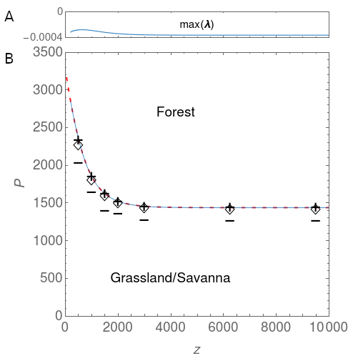
We made two types of figures: a phase plot with the front location in parameter space (Figure 1), and, scatterplots of cover types versus rainfall in the heterogeneous models (Figures 2 and 3). To create the phase plot of the heterogeneous models in Figure 1, we needed to extract the rainfall value at the front from the model output. For the simulations (markers in Figure 1), we did this via a robust curve fitting method, fitting the logistic function (goodness of fit $R^{2}>.9$ ),

F^{*}(P)=\frac{A}{1+\exp[-k(P-P_{f})]},

(7)

and extracting $P_{f}$ , with the MATLAB [17] curve fitting tool. In the numerical continuation of the heterogeneous forest model (solid blue line in Figure 1), we did this via

P_{f}=\arg\max F_{x}^{*}(P),

(8)

where $F_{x}^{*}$ is the spatial derivative of the front solution. We used (7) instead of (8) in the simulations because in the forest-savanna model, savanna species can induce gradients of $F$ away from the front. The two methods give the same results when there are no savanna trees (compare $+$ and solid blue line in Figure 1).

The analysis of the homogeneous model almost exclusively required symbolic analysis, which we did with Mathematica [18].

Results

In the first section below, we derive the MP of the homogeneous forest model. In the second section, the front pinning location in the heterogeneous forest model is derived via a numerical continuation. The third section shows simulation results of the heterogeneous forest and forest-savanna models.

Maxwell point of the homogeneous forest model

For simplicity we shall consider one spatial dimension, which gives rise to scalar fronts rather than domain boundaries in the form of line fronts. While the approach in 2D is identical once one chooses a direction of propagation of any invasion front, front dynamics will, unlike in 1D, be influenced by front curvature, but this is minimal for the spatial scales considered [19, 8]. Because we first assume forcing to be homogeneous, we can further treat $p$ and $z$ as parameters. We further also assume that the front width is very small compared to the domain size, such that it is justified to take the domain size as approximately infinite.

When starting from (6), hiding the dependence on $p$ and $z$ , grouping common factors, and indicating further $\partial_{t}u$ by $u_{t}$ and $\partial^{2}u/\partial x^{2}$ by $u_{xx}$ , we obtain

u_{t}=[\alpha-\beta u-f(u)]u+u_{xx}.

(9)

As the nonlinear term causes bistability, we expect traveling front solutions [see e.g. [20, 14, 13]] between the stable steady states of the form $u(\xi)$ with $\xi=x-ct$ and $c$ the wave speed, with boundary conditions $u(-\infty)=u_{-}$ and $u(\infty)=u_{+}$ such that we can rewrite our equation as

-cu^{\prime}=[\alpha-\beta u-f(u)]u+u^{\prime\prime},

where $u^{\prime}=du/d\xi$ and $u^{\prime\prime}=d^{2}u/d\xi^{2}$ . When multiplying by $u^{\prime}$ , we obtain

-c(u^{\prime})^{2}=[\alpha-\beta u-f(u)]uu^{\prime}+u^{\prime\prime}u^{\prime}.

Integrating this with respect to $\xi$ over the real axis, we further obtain

$\displaystyle-c\int_{-\infty}^{\infty}(u^{\prime})^{2}d\xi$	$\displaystyle=$	$\displaystyle\int_{-\infty}^{\infty}[\alpha-\beta u-f(u)]uu^{\prime}d\xi+\int_{-\infty}^{\infty}u^{\prime\prime}u^{\prime}d\xi,$
	$\displaystyle=$	$\displaystyle\int_{u_{-}}^{u_{+}}[\alpha-\beta u-f(u)]udu-\int_{u_{-}}^{u_{+}}u^{\prime}du^{\prime},$
	$\displaystyle=$	$\displaystyle\int_{u_{-}}^{u_{+}}[\alpha-\beta u-f(u)]udu-[\frac{1}{2}u^{\prime 2}]_{u_{-}}^{u_{+}}.$

As the solution is flat at the boundaries, we have $[\frac{1}{2}u^{\prime 2}]_{u_{-}}^{u_{+}}=0$ , such that

-c\int_{-\infty}^{\infty}(u^{\prime})^{2}d\xi=\int_{u_{-}}^{u_{+}}[\alpha-\beta u-f(u)]udu.

As the integrand of the left hand side of this expression is always positive, we have

\text{sign}(c)=\text{-sign}\{\int_{u_{-}}^{u_{+}}[\alpha-\beta u-f(u)]udu\}=\text{sign}(\Delta V),

(10)

where we have defined,

	$\displaystyle\Delta V$	$\displaystyle\equiv$	$\displaystyle-\int_{u_{-}}^{u_{+}}[\alpha-\beta u-f(u)]udu$
		$\displaystyle=$	$\displaystyle[-\alpha u^{2}/2+\beta u^{3}/3]_{u_{-}}^{u_{+}}+\int_{u_{-}}^{u_{+}}f(u)udu.$

Hence, we see that the dynamics can be derived from the potential by

u_{t}=-V_{u}+\nabla^{2}u.

At the MP, the front is stationary, i.e. $c=0$ , such that according to (10),

\Delta V=[-\alpha u^{2}/2+\beta u^{3}/3]_{u_{-}}^{u_{+}}+\int_{u_{-}}^{u_{+}}f(u)udu=0.

This allows calculation of an expression for the MP as a function of the parameters $\alpha$ and $\beta$ . These parameters, in turn, are a function of the external forcings of the model.

If we choose $f(u)$ as in (A1) with $Y=u$ ,

f(u)=\frac{u_{c}^{4}}{u_{c}^{4}+u{}^{4}},

(11)

then $\int f(u)du$ can be calculated analytically as

\int f(u)du=\frac{u_{c}^{2}}{2}\text{arctan}[\left(u/u_{c}\right)^{2}],

such that

V(u)=\frac{\beta u^{3}}{3}-\frac{\alpha u^{2}}{2}+\frac{u_{c}^{2}}{2}\text{arctan}[\left(u/u_{c}\right)^{2}].

$\Delta V=V(u_{+})-V(u_{-})$ can be found analytically if $u_{+}$ and $u_{-}$ can be found analytically. However, $u_{+},u_{-}$ can only be found analytically when the (integer) exponent in (A1) is $1\leq n\leq 3.$ As we chose $n=4$ , this step has to be done numerically. From here, the MP can be calculated by finding the root of $\Delta V$ as a function of its parameter(s). Also this is only possible numerically. The result of this calculation is shown as the dashed red line in Figure 1. For the parameters shown in Table 1, without human impact, and, at average rainfall seasonality and soils, the MP of the forest model lies at a mean annual rainfall of 1438mm. Areas receiving $P>1438\text{mm}$ will experience an invasion of forest while areas receiving $P<1438\text{mm}$ will experience loss of forest. When including human impact, forest is only considerably affected by human impact when it is less than $z\approx 2\text{km}$ away from agricultural areas.

Refer to caption — Fig 1: Maxwell point in the homogeneous forest model and pinning rainfall in the heterogeneous models. (A) Maximum eigenvalue of (14) for a range of $z$ values in the heterogeneous forest model (i.e. along the solid blue line in panel B). (B) Front between forest and savanna/grassland in $(P,z)$ space for different models. The dashed red line shows the theoretically derived MP from the homogeneous forest model and the solid blue line the location of the forest front in the heterogeneous forest model obtained by a numerical continuation. Markers show at which rainfall value the front settles in the heterogeneous models for given $z$ values: ( $+$ ) forest model (5), ( $\diamondsuit$ ) forest-savanna model (2) with $r_{S}=0.09$ and $Q_{0}=0.04$ , ( $-$ ) forest-savanna model (2) with $r_{S}=0.13$ and $Q_{0}=0.09$ .

Without spatial interaction in the forest model, there is a wide range where forest is bistable with grassland ( $\sim$ 1200-3500mm, upper branch and lower zero branch indicated with solid lines in Figure A1). Hence, we showed here that including spatial interaction causes the bistability range to collapse into one point - the MP. Note that when there are $N$ forcing variables, the MP is not a point but a $N-1$ dimensional surface in phase space. Away from the MP, the only stable state is the one with lowest potential energy $V$ . The alternative state with lower potential energy is now metastable. It can persist when: (1) the whole spatial domain is homogeneously in that state, and (2) that this homogeneous state is not sufficiently perturbed. Nonetheless, neither of these conditions are easily met in reality.

Front pinning in the heterogeneous forest model

When external conditions are heterogeneous, the parameters $p,z$ and the solutions $u_{+},u_{-}$ are functions of $x$ and the approach in the previous section cannot be used any more. However, one can expect that when the spatial dependence is weak, it can still be used as an approximation. It can then be expected that in the limit of $t\rightarrow\infty,$ areas receiving $P>P_{MP}$ will have forest while areas receiving $P<P_{MP}$ will not have forest, with the front pinned at $P_{MP}$ . The stability of the pinned front solution can be verified via a linear stability analysis. When writing the reaction term of (9) as ${\cal R}[u;P]$ , we have

u_{t}={\cal R}[u(x);P(x)]+u_{xx}.

(12)

At the front solution $u=u^{*}(x)$ , we perturb the solution with $\delta u(x,t)\ll 1$ and see how this perturbation grows by substituting $u^{*}(x)+\delta u(x,t)$ and neglecting higher order terms in $\delta u$ ,

$\displaystyle[u^{*}(x)+\delta u(x,t)]_{t}$	$\displaystyle=$	$\displaystyle{\cal R}[u^{}(x)+\delta u(x,t);P(x)]+[u^{}(x)+\delta u(x,t)]_{xx},$
$\displaystyle{}[\delta u(x,t)]_{t}$	$\displaystyle=$	$\displaystyle{\cal R}[u^{}(x);P(x)]+\frac{\partial{\cal R}}{\partial u}[u^{}(x),P(x)][\delta u(x,t)]+[u^{*}(x)+\delta u(x,t)]_{xx},$
$\displaystyle{}[\delta u(x,t)]_{t}$	$\displaystyle=$	$\displaystyle\frac{\partial{\cal R}}{\partial u}[u^{*}(x),P(x)][\delta u(x,t)]+[\delta u(x,t)]_{xx},$

where the second step is possible because ${\cal R}(u^{*};P)+u_{xx}^{*}=0$ as $u^{*}$ is a solution of (12). Therefore, the front solution is only stable with respect to perturbation when all eigenvalues of the operator,

{\cal L}(x)=\frac{\partial R}{\partial u}[u^{*}(x),P(x)]+\partial_{xx},

(13)

have negative real parts. In our case, it is not possible to obtain the front solution $u^{*}(x)$ analytically. Therefore, linear stability can be evaluated numerically, by calculating the eigenvalues of the discretized form of (13), which is the $n\times n$ matrix

\boldsymbol{{\cal L}}=\frac{\partial{\cal R}}{\partial u}(\mathbf{u}^{*},\mathbf{P})\mathbf{I}+\frac{\mathbf{L}}{\Delta x^{2}},

(14)

where $\mathbf{u}^{*}=[u(x_{0}),u(x_{1}),...,u(x_{n-1})]$ and $\mathbf{P}=[P(x_{0}),P(x_{1}),...,P(x_{n-1})]$ are the discretized front solution and rainfall values as a function of space, with $x_{k}=x_{0}+k\Delta x$ , $\mathbf{L}/\Delta x^{2}$ the discretized Laplacian, and $\mathbf{I}$ the identity matrix. If we define $\max\mathbf{v}$ as the maximum of a vector $\mathbf{v}$ ’s elements and $\boldsymbol{\lambda}$ as the vector with $n$ eigenvalues of (14), the condition for stability is hence

\max\Re(\boldsymbol{\lambda})<0,

(15)

where $\Re$ indicates that we take the real part. Because the front solution $\mathbf{u}^{*}$ depends on all the parameters, $\boldsymbol{{\cal L}}$ is calculated for only one point in parameter space. To obtain information on the stability of all front solutions in a given parameter range, one needs to obtain the solution for a set of points in that range and evaluate $\boldsymbol{{\cal L}}$ for each of them. Starting from a known front solution, pseudo-arclength continuation [21, 22, 23] allowed us to find other front solutions of (12) in parameter space. To compare the results with those of the previous section, we plot the rainfall value at which the front pins in the heterogeneous equation as a function of $z$ (distance from human cultivation). We extracted the location of the front via (8) for each value of $z$ . Our analysis shows that the front solution of the heterogeneous forest model (solid blue line in Figure 1) is indistinguishable from the MP of the homogeneous forest model (dashed red line in Figure 1). Moreover, we found that all for each value of $z$ considered (15) is satisfied (solid red line in Figure 1), indicating that each front solution is a stable steady state, or more specifically, a stable node, as all eigenvalues of (14) are real. It can hence be concluded that, at least for our setup with weak spatial dependence, the front of the heterogeneous forest equation pins at the MP of the homogeneous forest equation.

Simulation of the heterogeneous models

Here we show steady state profiles of vegetation by the heterogeneously forced models. We remind the reader that the used forcing is a linear relation between distance from the origin and rainfall (4) such that at the chosen left and right boundaries $P(0\text{km})=0\text{mm}$ and $P(3000\text{km})=3000\text{mm}$ , respectively. Therefore, the x-axis of the plots in Figure 2 and 3 is both distance from the origin in km or mean annual rainfall in mm.

Figure 2 shows the steady states of $F$ as a function of rainfall by the forest model (6) and of $S,T$ and $F$ by the forest-savanna model (2) for parameters leading to low savanna tree presence ( $r_{s}=0.09$ , $Q_{0}=0.04$ , $\tau=2.7$ ), with and without human impact. Without human impact, all models have their forest front pinned at a rainfall value of about 1400mm [Figure 2A (green), B (green)], with forest occurring above and grassland or savanna below this value. Adding human impact results in a shift of the forest front to higher rainfall values (2A blue versus green; 2C vs 2B). In the forest model, the MP obtained from the analysis of the homogeneous model (Figure 2, dashed lines without human impact and dash-dotted line with human impact) accurately predicts the location of the forest front (Figure 2A). The model with savanna trees (forest-savanna model) has its forest front at slightly lower rainfall values than the model without savanna trees (Figure 2C vs Figure 2B). The rainfall value at which the front pins is indicated by markers in Figure 1 for a wider range of $z$ values, confirming the good match [perfect match for the forest model ( $+$ ) and small bias for the forest-savanna model ( $\diamondsuit$ )] between the rainfall value at which the front pins and the MP of the homogeneous forest model for the parameters chosen here.

Figure 3A shows the cover types versus rainfall when we choose parameters leading to higher savanna tree cover ( $r_{s}=0.13$ , $Q_{0}=0.09$ ). As before, there is forest on the wet side and savanna on the dry side of the x axis. However, now adult savanna trees reach higher cover values and there is a larger difference between the MP and the location of the front (see $-$ markers in Figure 1 for a wider range of $z$ values). The MP becomes decreasingly accurate as predictor of the forest front with increasing savanna tree cover (Figure 3B versus 3A and 2D). Moreover, beyond the point where savanna cover decreases, there is a range of rainfall values below the forest front where forest and savanna tree cover show high variation due to irregular oscillations of forest and savanna tree cover (Figure 3D). Figure 3B shows that when savanna tree recruitment is increased further ( $Q_{0}=0.2$ ) and when also the fire return interval is decreased ( $\tau=1)$ , savanna tree cover becomes bistable below a rainfall of about 1000mm and the range of rainfall with forest-savanna cycles widens. We will further refer to the low savanna tree cover state as the savanna state and to the high savanna tree cover state the woodland state. Note that the savanna tree cover bistability also occurs (for the same parameters) without forest trees (Figure 3C,F), but up to a rainfall of about 2500mm.

In Figure 4, we show the forest-savanna cycles in more detail. During the cycles, forest tree cover lags behind savanna tree cover. The changes between states occur over decades, but the periods of stability between the transitions can persist for several centuries (or longer, depending on the parameters). The nonspatial system only produces a regular cycle (Figure 4A) while the spatially homogeneous system with diffusion (Figure 4B) has irregular cycles. The spatially heterogeneous system has similar irregular cycles (Figure 4C). The irregularity of these cycles can hence be induced by diffusion alone.

Discussion

In this paper, we have provided a first analytical and numerical analysis of our spatially heterogeneous reaction-diffusion model of tropical tree cover. We have treated this model before with a more realistic set-up [8] (in 2D, with noise and forced by observed climate, soil and human impact), but we formulated it here in an as simple as possible form (in 1D, deterministic and forced by linear rainfall) for easier mathematical analysis. The heterogeneity was captured with the relation (4), such that low x values represent dry and high x values represent wet areas. From the homogeneous system without savanna trees/saplings [ $S=T=0$ , (6)], a Maxwell point was derived. We showed via a numerical continuation and linear stability analysis of the spatially heterogeneous forest model that this MP is still of use for the spatially heterogeneous case because here, it is the parameter value at which the forest front pins. The MP of the homogeneous forest model and the rainfall value at which the forest model’s front pins as a function of external parameters (the dashed red line and the solid blue line in Figure 1 respectively) are indistinguishable and have the same shape as what was obtained in [8] by simulation. Existence of a MP in reaction-diffusion equation with a bistable reaction term [14, 20, 13] and pinning under heterogeneity [12] is consistent with previous work. For parameters that lead to low cover of savanna trees, the MP of (6) is also a good predictor of the forest-savanna model’s forest front [ $S,T\neq 0$ , (2)] (Figure 2C-F). This is because the effect of savanna trees on forest trees, mediated by burnt area [see (2)], remains negligible when savanna tree cover near the forest front stays below the threshold where fire spread is inhibited, i.e. $T<Y_{c}$ . Choosing parameters such that savanna tree cover near the forest front exceeds this threshold ( $T\apprge Y_{c}$ ) makes the forest front shift away from the MP of (6), towards drier areas (Figure 3A,B). In this regime where savanna tree cover affects forest tree cover, we also found forest-savanna cycles and savanna-woodland bistability, which both can lead to bimodal tree cover distributions under the same external forcings. These cycles are consistent with the existence of Hopf bifurcations in the nonspatial system [16] above a certain value of the parameters equivalent to $P$ and $r_{s}$ . For an explanation of the physical mechanism behind the cycles, we refer to [16]. We found that the cycles can turn irregular by diffusion. That the irregular cycles are produced endogenously suggests that close to the forest front, sudden and unpredictable loss of forest can occur without climatic or anthropogenic perturbations. We speculate that the irregularity is due to spatiotemporal chaos, which is known occur in the wake of traveling fronts [24, 25]. To prove this, it would need to be shown additionally that the cycles produced by the deterministic system are truly aperiodic and that there is sensitivity to initial conditions [26]. We further showed via simulation that bistability of a savanna and a woodland state can arise in the savanna model (i.e. the model without forest trees) under a regime of high sapling recruitment and high fire occurrence (Figure 3C,F). When introducing forest trees (under the same conditions), the savanna-woodland bistability does not survive at higher rainfall, due to competition between savanna and forest trees (Figure 3B). Instead, the irregular cycle discussed above appears. Where it is too dry for forest, savanna tree cover bistability does survive. To obtain a complete picture of the behavior of the spatial model and how it differs from the nonspatial model, its bifurcation diagrams need to be made. A step towards increased realism is then the consideration of two spatial dimensions instead of one, with a further step towards increased realism being the verification of how this diagram is affected by spatial heterogeneity.

Taking our results reported here together with the simulation results in our previous work [8] and other recent work [16], the forest-savanna model can produce bimodal tree cover distributions in a range of external parameters due to: (i) bistability between savanna and woodland, (ii) existence of forest-savanna cycles, (iii) spatial heterogeneity of forcings other than rainfall. Fitting our model for separate regions to data in empirically justified parameter ranges might reveal differences between different regions or suggest which model components are not adequately captured. That much of the tree cover bimodality in the Amazon region can be attributed to spatial heterogeneity, leaving little remaining bimodality [8], indicates on one hand that bistability and cyclic behavior play at most a small role in Amazonia. Nonetheless, dry forests in Amazonia and elsewhere might still exist as an alternative state to moist forest and/or savanna. In Africa, where there exist large areas of high tree cover savannas [27] and where fire occurrence is higher [11], bistability and cyclic behavior can be expected to play a larger role. A possibility other than the ones hitherto mentioned is that the observed bimodality is an artifact, resulting from data algorithms [28] or preprocessing methods [29]. Therefore, the multistability hypothesis should be tested on tree cover data produced with methods that are less likely to generate such artifacts.

Finally, there exist other types of feedbacks than assumed here and which can induce multistability. These include feedbacks between soil fertility and vegetation [30], rainfall and vegetation [31, 32, 33, 34], and, herbivore presence and vegetation. As all existing feedbacks may interact on various scales [35], there is no doubt that tropical vegetation is not just complex but also complicated. Nevertheless, the insight from complexity science that complicated dynamics can emerge from simple rules suggests that they might be less complicated than we currently think. In the search for such simple rules, spatiotemporal conceptual models like the one developed here will be indispensable. On the other hand, even if the rules turn out to be simpler than expected initially, their resulting dynamics may only be captured realistically when they are implemented in models that are sufficiently individual based.

Acknowledgments

We thank Jan Sieber for comments and Daniele Avitabile for sharing and explaining the MATLAB code for numerical continuation. For funding, BW and ARC acknowledge the UK EPSRC (BW: grant EP/N023544/1). JIH acknowledges the UK NERC (GGR Programme) and the EU FP7 (project LU4C).

Supporting Information

Appendix A Model construction

General overview

The model in space and time can be written as a system of stochastic partial differential equations of the reaction-diffusion type. In ecological context, one describes the dynamics of a species density as the sum of a reaction term, representing local demography, and a diffusion term, representing migration of the species through space from areas with high to areas with low density. Our model can be most compactly expressed in vector form

\displaystyle\partial_{t}\mathbf{Y}

\displaystyle=

\displaystyle\mathbf{J}(\mathbf{Y};\mathbf{A})+\mathbf{D}\nabla^{2}\mathbf{Y},

where $\mathbf{Y}=(S,T,F,G)$ with $S$ representing savanna sapling cover density, $T$ savanna tree cover density, $F$ forest tree cover density, and $G$ grass cover density. $\mathbf{A}$ is a vector of exogenous environmental variables or parameters that force the system, such as mean rainfall, rainfall seasonality and soils [8]. These forcing variables are in general all heterogeneous in space, but in the main text we kept rainfall seasonality and soils constant, and took mean annual rainfall as the only heterogeneous forcing. $\mathbf{J}$ is a vector of reaction terms representing local population dynamics involving both gains and losses and contains nonlinear terms in both $\mathbf{Y}$ and $\mathbf{A}$ . Note that one other forcing variable is contained in $\mathbf{J}$ , being human impact. With regards to qualitative dynamics and steady state distributions, the particular choices of the functional forms of $\mathbf{J}$ are arbitrary to some extent. As long as we choose the right shape, the phase portrait should be topologically equivalent to the true functional form. $\mathbf{D}$ is a diagonal matrix with diffusion constants. We take the forcing variables as constant in time. This is done by replacing $\mathbf{A}(\mathbf{x},t)$ by its long-term mean, which is only a function of space. We denote it further as $\mathbf{A}(\boldsymbol{x})=\mathbf{A}$ . We only consider 1D space here. Hence, $\nabla^{2}=\partial_{x}^{2}$ , $\mathbf{x}=x$ and $\mathbf{y}=y$ . In 2D, front dynamics will be influenced by front curvature but this is minimal for the spatial scales considered [19].

Local rates of change

Here, we show how the local rates of change $J_{Y}$ for $Y$ any of the cover types ( $S,T,F,G$ ) are chosen. As in any population model, we have

change

\displaystyle=

\displaystyle\text{gain}-\text{loss}

Below, the set of gain processes ${\cal P}_{G}$ contains recruitment and growth, while that of the loss processes ${\cal P}_{L}$ contains mortality from competition for resources, drought, fire and human impact. Each of those processes can be captured with a different term, such that the equations of the cover types $S,T,F$ and $G$ take the form

\dot{Y}=J_{Y}(\mathbf{Y};\mathbf{A})=\sum_{i\in{\cal P}_{G}}G_{Y,i}(\mathbf{Y};\mathbf{A})-\sum_{i\in{\cal P}_{L}}L_{Y,i}(\mathbf{Y};\mathbf{A},z).

As external climatic/edaphic forcing we choose

\mathbf{A}=(MAR,MSI,EFS),

where $MAR$ stands for the observed multi-annual mean of rainfall, $MSI$ Markham’s seasonality index and $EFS$ the edaphic suitability for forest [this lets our model agree with that of [8] but using a more compact notation]. $Y$ refers to any of the cover types. Functions $G_{Y,i}$ and $L_{Y,i}$ are respectively, total gains and total losses per time of species $Y$ by process $i$ . The functional forms will be chosen inspired by an understanding of the effect of all relevant processes.

Gain functions consist of

	$\displaystyle\sum_{i\in{\cal P}_{G}}G_{Y,i}(\mathbf{Y};\mathbf{A})$	$\displaystyle=$	$\displaystyle G_{Y,e}(\mathbf{Y};\mathbf{A})+G_{Y,r}(\mathbf{Y};\mathbf{A})+G_{Y,m}(\mathbf{Y};\mathbf{A}),$
			expansion, recruitment, mortality other types

Gains can occur due to local (subgrid) expansion of vegetation ( $i=e$ ), or, in case of an age-structured species, due to recruitment from a younger stage ( $i=r$ ), or due to increased availability of space after mortality of other cover types ( $i=m$ ). Loss functions consist of

	$\displaystyle\sum_{i\in{\cal P}_{L}}L_{Y,i}(\mathbf{Y};\mathbf{A})$	$\displaystyle=$	$\displaystyle L_{Y,r}(\mathbf{Y};\mathbf{A})+L_{Y,c}(\mathbf{Y};\mathbf{A})+L_{Y,d}(\mathbf{Y};\mathbf{A})+L_{Y,f}(\mathbf{Y};\mathbf{A})+L_{Y,h}(\mathbf{Y},z)+L_{Y,o}(\mathbf{Y})$
			recruitment, competition, drought, fire, humans, other

They can occur due to: recruitment to an older stage ( $i=r$ ), interspecific competition ( $i=c$ ), drought ( $i=d$ ), human impact ( $i=h$ ) or other causes ( $i=o$ ). Below, each of the gain/loss terms are discussed.

•

Cover gains and losses due to expansion. Gains due to expansion involve increase of cover area of a more competitive cover type at cost of the cover area of a less competitive type. Hence,

G_{Y,e}(\mathbf{Y};\mathbf{A})=R_{Y}(\mathbf{A})Y\mathbf{Y}.\mathbf{v}_{c,Y},

with $Y$ the species that expands its cover and $\mathbf{v}_{c,Y}$ the competitiveness vector for cover type $Y$ , which has ones at its elements where the corresponding cover type is less competitive than, and can be colonized by, $Y$ . The rationale is that colonization by a species occurs due to an interaction of the space that is occupied by that species with the space that can be colonized by it. Having chosen the competitive hierarchy $F>T>S>G$ [10] in absence of water limitation, we have

	$\displaystyle G_{F,e}(\mathbf{Y};\mathbf{A})$	$\displaystyle=$	$\displaystyle R_{S}(\mathbf{A})T\mathbf{Y}.\mathbf{v}_{c,S}=R_{F}(\mathbf{A})F(G+S+T),$
	$\displaystyle G_{S,e}(\mathbf{Y};\mathbf{A})$	$\displaystyle=$	$\displaystyle R_{F}(\mathbf{A})F\mathbf{Y}.\mathbf{v}_{c,F}=R_{S}(\mathbf{A})TG,$

These are removed from the areas of the less competitive types. Hence, losses due to expansion of competing types are

$\displaystyle L_{T,c}(\mathbf{Y};\mathbf{A})$	$\displaystyle=$	$\displaystyle R_{F}(\mathbf{A})TF$
$\displaystyle L_{S,c}(\mathbf{Y};\mathbf{A})$	$\displaystyle=$	$\displaystyle R_{F}(\mathbf{A})SF$
$\displaystyle L_{G,c}(\mathbf{Y};\mathbf{A})$	$\displaystyle=$	$\displaystyle R_{F}(\mathbf{A})GF+R_{T}(\mathbf{A})GT$

The only age-structured part of our model is that of savanna saplings $S$ and savanna (adult) trees $T.$ Note therefore that $G_{S,e}$ has $TG$ instead of $SG$ because expansion only comes from interaction of adult species $T$ with places that saplings $S$ can colonize ( $G$ ). The dependence of $R_{Y}$ on $\mathbf{A}$ captures the effect of water availability on growth, which we choose as

R_{Y}(\mathbf{A})=\max[0,r_{Y}(1-e^{-\mathbf{k_{R_{Y}}}.\mathbf{A}+a_{Y}})],

with $r_{Y}$ the maximal growth rate, $\mathbf{k_{R_{Y}}}$ as growth rate increase for every component of $\mathbf{A}$ and $a_{Y}$ fixing the rate for $\mathbf{A}=\boldsymbol{0}$ . This function captures saturation of growth rate where water limitation is less severe, which is supported by empirical work (e.g. saturation of NDVI as a function of rainfall and high temporal correlations between rainfall and NDVI below saturation; [36, 35]].

•

Gains and losses due to recruitment. Saplings will recruit into adults, such that,

$G_{T,r}(\mathbf{Y};\mathbf{A})=-L_{S,r}(\mathbf{Y};\mathbf{A})=Q(\Phi)S,$

where recruitment rate $Q$ is a function of burnt area fraction $\Phi$ ,

$Q(\Phi)=Q_{0}(1-h\Phi).$

$Q_{0}$ is the recruitment rate in absence of fire and $Q_{0}(1-h)$ the recruitment rate in presence of fire for a particular year, with $0\leq h\leq 1$ . Hence, in agreement with previous empirical work, fire affects the establishment rather than the mortality of savanna trees.
•

Base mortality. This is the base mortality in absence of fire, drought, competition or human impact. As is common in ecology, we choose this mortality linear in $Y$ ,

$L_{Y,o}=m_{Y,o}Y$

with $m_{Y,o}$ the base mortality rate of $Y$ .
•

Losses due to drought. Drought-related mortality rate $M_{Y}(\mathbf{A})$ will be chosen such that drought effects cause increased mortality below a certain threshold of $\mathbf{A}$ . We choose

$L_{Y,d}(Y;\mathbf{A})=M_{Y}(\mathbf{A})Y,$

with

$M_{Y}(\mathbf{A})=e^{-\mathbf{k_{M_{Y}}}.\mathbf{A}+a_{M_{Y}}},$

or when absorbing the base mortality rate into this term,

$M_{Y}(\mathbf{A})=m_{Y,o}+e^{-\mathbf{k}_{M_{Y}}.\mathbf{A}+a_{M_{Y}}}.$

Such nonlinear increase of mortality with dryness is assumed to be a consequence of exceedance of thresholds related to tree water availability.
•

Losses due to fire. $\Phi$ is burnt area fraction per year. Grasses and savanna tree saplings resprout very rapidly so they are assumed to be unaffected by fire on the considered time scale. Savanna trees are fire adapted so also they are also assumed to be unaffected by fire [10]. Hence, in this model, only forest trees experience direct mortality due to fire. This mortality is chosen proportional to burnt area and burning is assumed to occur in a homogeneously distributed fashion over the pixel. Thus

$L_{F,f}(\mathbf{Y};\mathbf{A})=b\Phi F,$

where $b$ is the fraction of fire affected forest that dies, also the fire sensitivity of forest cover. Previous research shows that fire in the tropics is determined by climate on large scales and by tree cover on small scales [4, and the references therein]. On the other hand, local-scale forest distribution affects fire occurrence. This means that forest and fire interact on local scales. Hence, a positive feedback can arise if this interaction occurs in a nonlinear fashion and if it reinforces changes. There exists evidence from independent lines of research for such positive feedbacks [4]. A fire feedback operating on small spatial scales is crucial for producing the two stable states, savanna and forest [10, 7, 37]. We parameterized the fire feedback by choosing burnt area fraction $\mathbb{F}$ as a sigmoid-shaped function of fire-prone cover, consistent with fire percolation models. We let this function further also depend on climate. The double-striked notation is used to distinguish it from the functions and variables related to the cover types. The fundamental process responsible for the fire feedback is small-scale spatial fire percolation over a fire prone layer. Simulations have shown [37] that this process induces a sharp increase of fire-related mortality around the percolation threshold, which occurs when about 60% of the landscape is fire-prone. We do not intend to model this percolation process but take a mesoscale approach, where we choose $\Phi(Y;\mathbf{A})$ to have a sharp increase around a total nonherbaceous cover $1-G-S=T+F=Y_{c}$ . Instead of modeling a positive threshold response of fire on fire-conductive cover ( $S+G$ ), we choose to formulate the functional form as a negative threshold response of fire on non-fire-conductive cover ( $T+F$ ). This makes the analysis easier while keeping the model qualitatively the same. We hence choose

$\Phi(T,F;\mathbf{A})=\frac{1}{\tau}\frac{Y_{c}(\mathbf{A})^{n}}{Y_{c}(\mathbf{A})^{n}+(T+F)^{n}}.$ (A1)

The exponent $n$ is a positive integer that controls the steepness of increase of burnt area fraction at $Y\approx Y_{c}$ . We chose $n=4$ . $Y_{c}(\mathbf{A})$ captures the varying percolation threshold with hydrological conditions - a lower threshold in drier environments. This dependence is chosen to be piecewise linear,

$Y_{c}(\mathbf{A})=\text{max}[0,Y_{c,0}+\mathbf{k}_{c}.\mathbf{A}].$

Here, $\mathbf{k}_{c}$ is a constant vector and $Y_{c,0}$ a constant scalar. The elements of $\mathbf{k}_{c}$ represent the sensitivity of $Y_{c}(\mathbf{A})$ to the different components of $\mathbf{A}$ . $Y_{c}$ has a value of about 40% for common conditions, which is the tree cover value at which fire has been observed to increase [38, 39, 8].
•

Losses due to human impact. Deforestation of forest trees is chosen as

$L_{F,h}(F,z)=C(z)F,$

where $C(z)$ is the deforestation rate and $z$ distance from anthropogenically impacted areas. We choose

$C(z)=ce^{-k_{C}z},$

such that the deforestation rate decays with distance from impacted areas. $c$ is the the maximum deforestation rate, which occurs in agricultural areas ( $z=0$ ).
•

Gains due to mortality of other cover types. When any cover type loses space, it makes place for other cover types. When this does not occur due to competition or recruitment, grass is the default cover type that gains ground. This agrees with taking the assumption that grass grows back instantly, which was also taken in [10]. Therefore,

$G_{G,m}(\mathbf{Y};\mathbf{A})=\sum_{\begin{array}[]{c}Y\in\{S,T,F\}\\ i\in\{d,f,h,o\}\end{array}}L_{Y,i}(\mathbf{Y};\mathbf{A}),$

of which the terms are defined above.

The system of equations locally obeys the aforementioned mathematical constraint for every point in time

\sum_{Y\in\{S,T,F,G\}}Y=1.

Differentiation of the above equation with respect to time yields

	$\displaystyle\sum_{Y\in\{S,T,F,G\}}\partial_{t}Y$	$\displaystyle=$	$\displaystyle 0,$
	$\displaystyle\sum_{Y\in\{S,T,F,G\}}J_{Y}(\mathbf{Y};\mathbf{A})$	$\displaystyle=$	$\displaystyle 0.$		(A2)

The conservation equation A2 implies that the sum of all loss and gain terms should be zero. We can see that this is the case because: (i) total expansion due to successful competition is at the cost of total loss due to unsuccessful competition, (ii) recruitment lost by $S$ is gained by $T$ , (iii) tree cover losses due to fire, drought and human impact are gained by grass cover.

Spatial dependence

Thus far, we have only treated the dynamics as spatially independent [ $\mathbf{Y}=\mathbf{Y}(t)$ ], for particular parameter values of hydrology $\mathbf{A}$ and distance to human impacted areas $z$ . To run this model for a whole region [ $\mathbf{Y}=\mathbf{Y}(\mathbf{x},t)$ ], we need to take into account not only the spatial heterogeneity of these variables but also the relevant spatial interactions.

1.

Spatial heterogeneity. Climatic, edaphic and anthropogenic spatial heterogeneity can be included by taking $\mathbf{A}$ and $z$ as functions of space $\mathbf{A}(\mathbf{x})$ and $z(\mathbf{x})$ .
2.

Spatial interaction. We assume that diffusion of cover types only occurs due to spread of seeds. We do not model seed dispersal but approximate it by dispersal of saplings. Hence the diffusion coefficient of savanna adult tree cover is zero. That of forest cover is not zero because part of its population is in the sapling stage. Hence,

$\mathbf{D}=(D_{S},0,D_{F},0).$

The cover types that diffuse from neighboring areas settle in the areas that are taken by grasses. Therefore, in the spatial model, the diffusion terms are also grass cover loss terms due to unsuccessful competition, or

$L_{G,c}(\mathbf{Y};\mathbf{A})=R_{F}(\mathbf{A})GF+R_{T}(\mathbf{A})GT+D_{S}\nabla^{2}S+D_{F}\nabla^{2}F.$

Spatial interaction can also occur due to spread of fire. While analysis of the model with fire spread is less straight forward [19], the conclusions are the same.

Forest-savanna model

Here, we develop the forest-savanna model with all previously mentioned cover types. Note that we do not write the explicit dependence on space and time. Hence, this means that all cover types are a function of space $\mathbf{x}$ and time $t$ . The forcings are only a function of space, i.e. $\mathbf{A}=\mathbf{A}(\mathbf{x})$ and $z=z(\mathbf{x})$ . Based on the previous sections, we have

$\displaystyle\partial_{t}S$	$\displaystyle=$	$\displaystyle G_{S,e}(\mathbf{Y};\mathbf{A})-L_{S,r}(\mathbf{Y};\mathbf{A})-L_{S,d}(S;\mathbf{A})-L_{S,c}(\mathbf{Y};\mathbf{A})+D_{S}\nabla^{2}S,$
$\displaystyle\partial_{t}T$	$\displaystyle=$	$\displaystyle G_{T,r}(\mathbf{Y};\mathbf{A})-L_{T,d}(T;\mathbf{A})-L_{T,c}(\mathbf{Y};\mathbf{A}),$
$\displaystyle\partial_{t}F$	$\displaystyle=$	$\displaystyle G_{F,e}(\mathbf{Y};\mathbf{A})-L_{F,d}(F;\mathbf{A})-L_{F,f}(\mathbf{Y};\mathbf{A})-L_{F,h}(F,z)+D_{F}\nabla^{2}F,$
$\displaystyle\partial_{t}G$	$\displaystyle=$	$\displaystyle-L_{G,c}(\mathbf{Y};\mathbf{A})+G_{G,m}(\mathbf{Y};\mathbf{A}),$

Filling in the gains and losses and making use of $G=1-S-T-F$ , we obtain

$\displaystyle\partial_{t}S$	$\displaystyle=$	$\displaystyle R_{s}(\mathbf{A})(1-S-T-F)T-Q[\Phi(T,F;\mathbf{A})]S-M_{S}(\mathbf{A})S-R_{F}(\mathbf{A})SF,$
$\displaystyle\partial_{t}T$	$\displaystyle=$	$\displaystyle Q(\Phi)S-M_{T}(\mathbf{A})T-R_{F}(\mathbf{A})TF,$
$\displaystyle\partial_{t}F$	$\displaystyle=$	$\displaystyle R_{F}(\mathbf{A})(1-F)F-b\Phi(T,F;\mathbf{A})F-M_{F}(\mathbf{A})F-C(z)F+D_{F}\nabla^{2}F,$

We briefly remind the reader of some of the model parameters shown here. This model is forced by the spatial distribution of $\mathbf{A}$ and the distance to human impact $z$ . $b$ is the (constant) sensitivity of forest cover to fire. $Q$ represents sapling recruitment into adults and is a linearly decreasing function of burnt area fraction. $C(z)$ is the deforestation rate which decays with $z$ . Note that the simulation model used to produce Figure 1A has no deforestation term in the equation of $\partial_{t}T$ . When hiding the dependence on $\mathbf{A}$ , we have

$\displaystyle\partial_{t}S$	$\displaystyle=$	$\displaystyle R_{s}(1-S-T-F)T-Q[\Phi(T,F)]S-M_{S}S-R_{F}SF+D_{S}\nabla^{2}S,$
$\displaystyle\partial_{t}T$	$\displaystyle=$	$\displaystyle Q[\Phi(T,F)]S-M_{T}T-R_{F}TF,$
$\displaystyle\partial_{t}F$	$\displaystyle=$	$\displaystyle R_{F}(1-F)F-b\Phi(T,F)F-M_{F}F-C(z)F+D_{F}\nabla^{2}F,$	(A3)

Appendix B Forest growth rate $r_{F}$

Here, we will show how we derived the maximum forest growth rate. We do this to set the time scale of the model dynamics (other parameters were initially estimated relative to $r_{F}$ ). The steady state forest cover value under sufficiently moist conditions is about 80%. Therefore, we made sure that this also occurs in the model by first seeing that in moist conditions far from human-impacted areas, $C_{F}=0$ , $\Phi=0$ , $R_{F}=r_{F}$ and $M_{F}=m_{F,o}$ such that

\displaystyle\frac{dF}{dt}

\displaystyle=

\displaystyle r_{F}(1-F)F-m_{F,o}F.

We will further set $m_{F,o}\equiv m$ and $r_{F}\equiv r$ . The ODE can be solved by separation of variables using partial fractions such that the time that forest needs to grow from $F_{0}$ to $F_{1}>F_{0}$ is

t_{1}-t_{0}=\frac{1}{r(1-m)}\text{log}(\frac{\left|1-m-F_{0}\right|F_{1}}{\left|1-m-F_{1}\right|F_{0}}).

(A4)

If we take as initial tree cover a small value that could result from noise and as final tree cover the carrying capacity, we have

\displaystyle F_{0}

\displaystyle=

\displaystyle 0.01,\;F_{1}=0.8.

At carrying capacity, we have $r(1-F)F-mF=0,$ such that

F^{*}=1-\frac{m}{r},\;F^{*}=0.

of which only the first is stable. As the data shows that $F^{*}$ has to be equal to $0.8$ , such that $m=0.2r$ . Substituting this and the values for $F_{0},F_{1}$ , we obtain

t_{1}-t_{0}=\frac{1}{r(1-0.2r)}\text{log}(400\frac{0.99-0.2r}{1-r}).

(A5)

This function is plotted in Figure A2. In a recent study on recovery of secondary forests [40], it was found that moist forests regain the median value of old-growth forests after about at least 30 years. Therefore, we chose the $r$ value consistent with this time, which is

r\approx 0.2.

Supplementary Table

process and equation

value

parameter

units

cover expansion rate

0.09,0.20

r_{S},r_{F}

\text{y}^{-1}

R_{Y}(\mathbf{A})=\max[0,r_{Y}(1-e^{-\mathbf{k_{R_{Y}}}.\mathbf{A}+a_{R_{Y}}})]

(0.005,-,-)

\mathbf{k}_{R_{S}}

(\text{mm${}^{-1}$},\text{-,-})

(0.003,3.26,-)

\mathbf{k}_{R_{F}}

(\text{mm${}^{-1}$},\text{-,-})

0.25,0.196

a_{R_{S}},a_{R_{F}}

cover reduction rate by drought

0.023,0.041

m_{S,o}=m_{T,o},m_{F,o}

y^{-1}

M_{Y}(\mathbf{A})=m_{Y,o}+e^{-\mathbf{k}_{M_{Y}}.\mathbf{A}+a_{M_{Y}}}

-,-2.15

a_{M_{S}}=a_{M_{T}},a_{M_{F}}

(0.008,-,-)

\mathbf{k}_{M_{S}}=\mathbf{k}_{M_{T}}

(\text{mm${}^{-1}$},\text{-,-})

(0.008,-4.66,1.5)

\mathbf{k}_{M_{F}}

(\text{mm${}^{-1}$},\text{-,-})

savanna tree cover recruitment rate

Q(\Phi)=Q_{0}(1-h\Phi)

0.04,0.85

Q_{0},h

\text{y}^{-1},\text{-}

local burnt area fraction

\Phi(T,F;\mathbf{A})=\frac{1}{\tau}\frac{Y_{c}(\mathbf{A})^{n}}{Y_{c}(\mathbf{A})^{n}+(T+F)^{n}},

2.7,4

\tau,n

\text{y}^{-1},\text{-}

with:

Y_{c}(\mathbf{A})=\text{max}[0,Y_{c,0}+\mathbf{k}_{c}.\mathbf{A}]

0.484

Y_{c,0}

(-1.43e-04,.2,-.1)

\mathbf{k}_{c}

(\text{mm${}^{-1}$},\text{-,-})

forest cover fire sensitivity

0.46

b

deforestation rate

C(z)=ce^{-k_{C}z}

0.092,0.0015

c,k_{C}

\text{m}^{-1}

diffusion coefficient of

F,S

0.1,0.2

D_{F},D_{S}

\text{km}^{2}\text{y}^{-1}

Table A1: Model parameters of the forest-savanna model [equation (A3)].

\mathbf{A}=\mathbf{A}(\mathbf{x})

. The components of are:

A_{1}=P

(mean annual rainfall),

A_{2}=M

(Markham’s seasonality index),

A_{3}=\pi-\bar{\pi}

(edaphic forest suitability).

\pi

captures the effect of soils on forest occurrence and is taken from [8], i.e.

A_{3}=0.00238\varphi_{s}-0.188\varphi_{c}-5.99\rho-0.183\varphi_{c}\rho+6.39

, where

\rho

is topsoil bulk density,

\varphi_{s}

topsoil sand fraction, and

\varphi_{c}

topsoil clay fraction. The components of the vectors

\boldsymbol{k}_{i}

multiply the components of

\mathbf{A}

. If a component is indicated as ’-’, the considered equation is not a function of the corresponding component of

\mathbf{A}

Supplementary Figures

Literature Cited

1. Townshend JRG, Carroll ML, DiMiceli CM, Sohlberg RA, Hansen MC, DeFries R. type [; 2011]Available from: https://lpdaac.usgs.gov/dataset_discovery/modis/modis_products_table/mod44b.
2. Hirota M, Holmgren M, van Nes EH, Scheffer M. Global Resilience of Tropical Forest and Savanna to Critical Transitions. Science. 2011;334(6053):232–235. doi:10.1126/science.1210657.
3. Staver AC, Archibald S, Levin SA. The Global Extent and Determinants of Savanna and Forest as Alternative Biome States. Science. 2011;334(6053):230–232. doi:10.1126/science.1210465.
4. Pausas JG, Dantas VdL. Scale matters: fire–vegetation feedbacks are needed to explain tropical tree cover at the local scale. Global Ecology and Biogeography. 2017;26(4):395–399. doi:10.1111/geb.12562.
5. Ratajczak Z, Nippert JB. Comment on “Global Resilience of Tropical Forest and Savanna to Critical Transitions”. Science. 2012;336(6081).
6. Good P, Harper A, Meesters A, Robertson E, Betts R. Are strong fire-vegetation feedbacks needed to explain the spatial distribution of tropical tree cover? Global Ecology and Biogeography. 2016;25(1):16–25. doi:10.1111/geb.12380.
7. van Nes EH, Hirota M, Holmgren M, Scheffer M. Tipping points in tropical tree cover: linking theory to data. Global Change Biology. 2014;20(3):1016–1021. doi:10.1111/gcb.12398.
8. Wuyts B, Champneys AR, House JI. Amazonian forest-savanna bistability and human impact. Nature Communications. 2017;8(May):15519. doi:10.1038/ncomms15519.
9. Staal A, Dekker SC, Xu C, van Nes EH. Bistability, Spatial Interaction, and the Distribution of Tropical Forests and Savannas. Ecosystems. 2016;19(6):1080–1091.
10. Staver AC, Levin SA. Integrating theoretical climate and fire effects on savanna and forest systems. The American Naturalist. 2012;180(2):211–224.
11. van Nes EH, Staal A, Hantson S, Holmgren M, Pueyo S, Bernardi RE, et al. Fire forbids fifty-fifty forest. PloS One. 2018;13(1):e0191027. doi:10.1371/journal.pone.0191027.
12. Van De Leemput IA, van Nes EH, Scheffer M. Resilience of alternative states in spatially extended ecosystems. PloS one. 2015;10(2):1–17. doi:10.1371/journal.pone.0116859.
13. Meron E. Nonlinear physics of ecosystems. CRC Press; 2015.
14. Murray JD. Mathematical biology. I: An Introduction, volume 17 of Interdisciplinary Applied Mathematics. Springer-Verlag, New York; 2002.
15. Huang K. Introduction to statistical physics. CRC press; 2009.
16. Touboul JD, Staver AC, Levin SA. On the complex dynamics of savanna landscapes. Proceedings of the National Academy of Sciences. 2018; p. 201712356. doi:10.1073/pnas.1712356115.
17. MathWorks. type [; 2012]Available from: uk.mathworks.com.
18. Wolfram Research Inc. type [; 2018].
19. Wuyts B, Champneys AR, House JI. Bistability of Tropical Vegetation in a Heterogeneous Environment [PhD thesis]. University of Bristol; 2017.
20. Pismen LM. Patterns and interfaces in dissipative dynamics. Springer Science & Business Media; 2006.
21. Avitabile D. Numerical calculation of coherent structures in spatially-extended neural networks; 2016. Available from: https://icmns2016.inria.fr/pre-conference-workshop/.
22. Rankin J, Avitabile D, Baladron J, Faye G, Lloyd DJB. Continuation of localised coherent structures in nonlocal neural field equations. SIAM Journal on Scientific Computing. 2013;36(1):B70–B93. doi:10.1137/130918721.
23. Beyn WJ, Champneys A, Doedel E, Govaerts W. Numerical continuation, and computation of normal forms. Handbook of Dynamical Systems. 2000;.
24. Sherratt JA, Lewis MA, Fowler AC. Ecological chaos in the wake of invasion. Proceedings of the National Academy of Sciences of the United States of America. 1995;92(7):2524–8.
25. Sherratt JA, Smith MJ. Periodic travelling waves in cyclic populations: field studies and reaction-diffusion models. Journal of the Royal Society, Interface. 2008;5(22):483–505. doi:10.1098/rsif.2007.1327.
26. Strogatz SH. Nonlinear dynamics and chaos: with applications to physics, biology, chemistry, and engineering. Westview press; 2014.
27. Grainger A. Constraints on modelling the deforestation and degradation of tropical open woodlands; 1999. Available from: http://www.jstor.org/stable/2997881.
28. Hanan NP, Tredennick AT, Prihodko L, Bucini G, Dohn J. Analysis of stable states in global savannas: is the CART pulling the horse? Global Ecology and Biogeography. 2014;23(3):259–263. doi:10.1111/geb.12122.
29. Gerard F, Hooftman D, van Langevelde F, Veenendaal E, White SM, Lloyd J. MODIS VCF should not be used to detect discontinuities in tree cover due to binning bias. A comment on Hanan et al. (2014) and Staver and Hansen (2015). Global Ecology and Biogeography. 2017;26(7):854–859. doi:10.1111/geb.12592.
30. Paiva AO, Silva LCR, Haridasan M. Productivity-efficiency tradeoffs in tropical gallery forest-savanna transitions: linking plant and soil processes through litter input and composition. Plant Ecology. 2015;216(6):775–787. doi:10.1007/s11258-015-0466-8.
31. Eltahir EAB, Bras RL. Precipitation recycling in the Amazon basin. Quarterly Journal of the Royal Meteorological Society. 1994;120(518):861–880. doi:10.1002/qj.49712051806.
32. Pielke RA. Influence of the spatial distribution of vegetation and soils on the prediction of cumulus Convective rainfall. Reviews of Geophysics. 2001;39(2):151–177. doi:10.1029/1999RG000072.
33. Pöschl U, Martin ST, Sinha B, Chen Q, Gunthe SS, Huffman JA, et al. Rainforest aerosols as biogenic nuclei of clouds and precipitation in the Amazon. Science (New York, NY). 2010;329(5998):1513–6. doi:10.1126/science.1191056.
34. Zemp DC, Schleussner CF, Barbosa HMJ, Hirota M, Montade V, Sampaio G, et al. Self-amplified Amazon forest loss due to vegetation-atmosphere feedbacks. Nature Communications. 2017;8:14681. doi:10.1038/ncomms14681.
35. Scheffer M, Holmgren M, Brovkin V, Claussen M. Synergy between small-and large-scale feedbacks of vegetation on the water cycle. Global Change Biology. 2005;11(7):1003–1012. doi:10.1111/j.1365-2486.2005.00962.x.
36. Wuyts B, Govers G. A System Perspective on Sahel Greening [MSc Thesis]. University of Leuven; 2012.
37. Schertzer E, Staver AC, Levin SA. Implications of the spatial dynamics of fire spread for the bistability of savanna and forest. Journal of Mathematical Biology. 2015;70(1-2):329–341. doi:10.1007/s00285-014-0757-z.
38. Archibald S, Roy DP, van Wilgen BW, Scholes RJ. What limits fire? An examination of drivers of burnt area in Southern Africa. Global Change Biology. 2009;15(3):613–630. doi:10.1111/j.1365-2486.2008.01754.x.
39. Staver AC, Archibald S, Levin S. Tree cover in sub-Saharan Africa: Rainfall and fire constrain forest and savanna as alternative stable states. Ecology. 2011;92(5):1063–1072. doi:10.1890/i0012-9658-92-5-1063.
40. Poorter L, Bongers F, Aide TM. Biomass Resilience of Neotropical Secondary Forests. Nature. 2016;530(7589):211–227.

Update 05/2021: Gradient system requirement

Abstract

Introduction

Methods

Forest-savanna model

Forest model (S,T=0)

Parameters, simulation and figures

Results

Maxwell point of the homogeneous forest model

Front pinning in the heterogeneous forest model

Simulation of the heterogeneous models

Discussion

Acknowledgments

Appendix A Model construction

General overview

Local rates of change

Spatial dependence

Forest-savanna model

Appendix B Forest growth rate rFr_{F}

Supplementary Table

Supplementary Figures

Literature Cited

Appendix B Forest growth rate $r_{F}$