Discrete Potts Model for Generating Superpixels on Noisy Images

The main tools for denoising are variational methods like the approach with Potts priors [10], which was designed to preserve sharp discontinuities (edges) in images while removing noises. While in this paper, we point out that the discrete Potts model can be also applied for image segmentation.

Denote the input intensity values (color or gray-scale value) of pixels as $Y=(y_{ij})$. Since we are working on a grid graph, we denote the $i$-th row of $Y$ by $Y^{r}_{i}$ and the $j$-th column by $Y^{c}_{j}$. Let $W=(w_{ij})\in\mathbb{R}^{m\times n}$ be the fitting (denoised) value of pixels (Similarly we have $W^{r}_{i}$ and $W^{c}_{j}$). We divide $E=E^{r}\cup E^{c}$ into its horizontal (row) edges $E^{r}$ and its vertical (column) edges $E^{c}$. The classical (discrete) Potts model has the form

where the first two terms measure the $\ell_{k}$ norm difference between every row and column vector of $W$ and $Y$, and the further terms measure the number of oscillations in $W$ per row and column. Recall that the discrete first derivative $\nabla^{1}\mathbf{w}$ of a vector $\mathbf{w}\in\mathbb{R}^{n}$ is defined as the $n-1$ dimensional vector $(w_{2}-w_{1},w_{3}-w_{2},\ldots,w_{n}-w_{n-1})$ and the $\ell_{0}$ norm of a vector gives the number of its nonzero entries. The scalar $\lambda$ is a parameter for regularization.

In general, solving the discrete Potts model (1) is $\mathcal{NP}$-hard, and [11] uses local greedy methods. Recently, a MILP formulation is applied in [12] to deal with the $\ell_{0}$ norm for a similar problem in statistics called the best subset selection problem.

Since $G$ in $2$D is a grid graph, $E^{r}=\{E^{r}_{1},E^{r}_{2},\ldots,E^{r}_{m}\}$, where $E^{r}_{i}$ is the set of horizontal edges in the $i$-th row. Similarly, we have $E^{c}=\{E^{c}_{1},E^{c}_{2},\ldots,E^{c}_{n}\}$. We propose to formulate problem (1) as a MILP by introducing $m\cdot(n-1)+(m-1)\cdot n$ binary edge variables $x_{e}$. We would like the following properties to hold

where $\nabla^{1}w_{e}:=w_{h_{e}}-w_{t_{e}}$, and $h_{e}$, $t_{e}$ denotes the two end nodes of any edge $e\in E$. We call an edge $e\in E$ active if $x_{e}=1$, otherwise it is dormant.

In $1$D, if the above condition holds, nodes within two active edges will have the same intensity, while the two end nodes of an active edge have different. It thus corresponds to a piecewise linear constant fitting problem, see left part of Fig. 2 for an example.

A mixed integer programming (MIP) formulation for (1) that satisfies properties (2) reads

where $[m]$ denotes the discrete set $\{1,\ldots,m\}$ and $M$ should be big enough so that (a,b) are always valid when $|\nabla^{1}w_{e}|\neq 0$. Note that we use the $\ell_{1}$ norm over $\ell_{2}$ because it is more robust to outliers. Secondly, it is easier to model the $\ell_{1}$ with linear constraints, where constraint (a) is replaced by the two constraints $\nabla^{1}w_{e}\leq Mx_{e}$ and $-\nabla^{1}w_{e}\leq Mx_{e}$. The term $|w_{ij}-y_{ij}|$ is replaced by $\varepsilon_{ij}^{+}+\varepsilon_{ij}^{-}$ where $w_{ij}-y_{ij}=\varepsilon^{+}_{ij}-\varepsilon^{-}_{ij}$ and $\varepsilon_{ij}^{+},\varepsilon_{ij}^{-}\geq 0.$ In this paper, for simplicity, we will just specify models in form (3).

The proof can be found in the supplementary materials.

The multicut problem (Multicuts) in [13] formulates the image segmentation problem as an edge labeling problem. For a partition ${\cal V}=\{V_{1},V_{2},\ldots,V_{k}\}$ of $V$, the edge set $\psi(V_{1},V_{2},\ldots,V_{k})=\{uv\in E\mid\exists i\neq j\text{ with }u\in V_{i}\text{ and }v\in V_{j}\}$ is called the multicut induced by $\cal V$. Similar to the previous section, we introduce binary edge variables $x_{e}$ and the multicut is just a set of active edges.

With edge weights $c:E\rightarrow\mathbb{R}$ typically representing differences between pixels’ intensities, the multicut problem for the unsupervised image segmentation [14] can be formulated as the following integer linear program (ILP)

where $\lambda$ serves as the penalty term for the number of active edges. Constraints (a) are called the multicut constraints and they enforce the consecutiveness of the active edges, and thus the connectedness of each segment. Thus, a segment is composed with the maximal set of vertices induced only by the dormant edges. See the right part of Fig. 2, where the dashed edges form the multicut.

It is well known that if a cycle $C\in G$ is chordless, then the corresponding constraint (a) is facet-defining for the multicut polytope [14]. However, the number of such inequalities is exponentially in $|V|$, and they are usually added iteratively using a cutting plane method.

It is common practice to add additional constraints to a MIP for computational efficiency. A violating constraint “cuts off” feasible solutions of a formulation, which are not optimal. A constraint is redundant if it is not necessarily needed for a formulation to be valid. However, they may be useful because they forbid some fractional solutions during the branch-and-bound approach, where the MIP solver iteratively solves the linear programming (LP) relaxation.

Let $S:=\{(\mathbf{w},\mathbf{x})\;|\;(\mathbf{w},\mathbf{x})\text{ is feasible to problem~\eqref{eq:Pott_1D2}}\}$ be the set of all feasible solutions to (3), and $S_{I}:=\{\mathbf{x}\subset(\mathbf{w},\mathbf{x})\;|\;(\mathbf{w},\mathbf{x})\in S\}$ denotes its projection to $\mathbf{x}$. Denote $S^{o}\subseteq S$, where $(\mathbf{w},\mathbf{x})\in S^{o}$ satisfies property 2, and we let $S_{I}^{o}$ be the projection of $S^{o}$ to $\mathbf{x}$.

The proof can be found in the supplementary materials.

Note that the multicut constraints (a) are not always valid for the feasible set of (3), one example is shown in the supplementary materials. Since we know the multicut uniquely defines an image segmentation, we can now conclude that the optimal solution of the discrete Potts model (3) also defines a unique segmentation.

The proof can again be found in the supplementary materials.

Inspired by the multicut problem (4), in a grid graph, although the number of multicut constraints is still exponential, it may be advantageous to add the following $4$-edge chordless cycle (e.g., cycle $e_{0}$-$e_{1}$-$e_{2}$-$e_{3}$ in Fig. 2) constraints

to (3). Because it is the simplest (in terms of the number of edges) chordless cycle in a grid graph, plus the number of such constraints is only linear in $|E|$.

Of course, there exists more complicated strategy on selecting such cuts, which is beyond the focus of this paper. Interested readers may refer to [15, 16, 17] for more information. We will show experiments in Sec. 3 on the effects of adding the above constraints.

The main formulation (PMcut) is obtained by adding (5) into (3), which could be seen as an extension of [18] from discrete to continuous labeling space (if we treat $w_{i}$ as the label of node $i$). Note that by placing penalty term $\lambda$ on each actives edge, it in turn penalizes the length of segment boundary, thus encouraging compact shape of the segmentation. Upon solving (3), variable $x_{e}$ gives the boundaries of each segment, and $w_{ij}$ is the denoised value for every pixel. Thus, we get both segmentation and denoising of the input image.

PMcut is then solved using any standard off-the-shelf MIP solver, where advanced branch-and-cut methods are employed. One can set limits on the running time or the MIP gap. The MIP solver could return the best feasible solution found and the MIP gap upon termination.

All the computational experiments in this paper were performed using a commercial MIP solver Gurobi $7.5.1$, on an Intel i5-4570 quad-core desktop, with 16GB RAM. If the input image is RGB, we first transform it into gray-scale valued image, and normalize the intensity of each pixel to $[0,1]$.

Note that we choose to work on gray-scale mainly due to computational reasons. In theory, PMcut can be easily adapted to RGB images, by introducing continuous fitting variables $w$ for every channel. But this will trigger $O(mn)$ more variables and constraints.

For visualization, we take an image from [19], resize it to $40\times 40$, and add Gaussian and Salt and Pepper (S&P) noise with a time limit of $50$ secs.

Parameter setting. We simply set the constant $M$ to be $1$, so that (a,b) are always valid. We compute the average intensity of each $5\times 5$ pixel block of the image, and then calculate the absolute difference of their maximum and minimum value, denoted $Y^{*}$. So $Y^{*}$ somehow represents the global contrast of the image. Since we assume the input image contains noise, the regularization parameter is set to $\lambda=\frac{1}{4}\sigma Y^{*}$, where $\sigma$ is a user-defined parameter. When there exists an outlier, PMcuts will not treat the outlier as a one-pixel segment, since doing so would incur the penalty $4\lambda$ (equals $\sigma Y^{*}$).

Multicuts VS PMcut. The right part of Fig. 3 shows the input image, the detailed setting of the parameters and segmentation results. The first two columns are Multicuts with different $\lambda$. The third column represents PMcut. The number of segments is reported in Fig. 3. Multicuts takes less than one sec in all three instances. Although found optimal solution of the first instance in less than 6 sec, PMcut did not converge in the second instance with the time limit. The MIP gap is $1.91\%$.

With and without constraints (5). We report that with (5), PMcut saves $0.9$ secs in the first instance, and narrows down $23.5\%$ of the MIP gap in the second one, compared to without (5). We conduct $10$ more experiments (size $40\times 50$, with $5\%$ $S\&P$ noise, time limit $50$ secs), and report that these constraints help reduce the MIP gap from $66\%$ to $37\%$ on average.

We can conclude that it is hard to control the desired number of segments for Multicuts. On the other hand, although requiring more computational time, PMcut is robust to noise, easier to control parameters, and give better segmentation results. Also, it is clearly beneficial to add constraints (5) to the Potts (3), as we did in PMcut.

Our superpixel algorithm is quite straightforward. We begin by first decomposing the input image into $K$ rectangular patches, where $K$ is a user defined parameter approximating the number of desired superpixels. We then apply PMcut within each image patch. The superpixel is also upper bounded by the size of the patch.

Since PMcut is $\mathcal{NP}$-hard, smaller patches are desired for the sake of computational efficiency. In practice, we notice that with the increase of the number of patches, the overall computational time decreases since the patch size shrinks.

Note also that every image patch can be computed separately, thus parallelism can be fully adopted. In practice, one can also set a MIP gap threshold for PMcut within each patch. As a matter of fact, we often notice the segmentation results are already quite good even though it has not reached the optimal solution. Hence it makes sense to create a stopping criterion when PMcut either hits a time limit or it finds a solution within a certain MIP gap. We set the threshold of MIP gap to $2\%$ in later experiments.

Among other metrics, the Under-segmentation Error (UE), Boundary Recall (Rec) and Compactness (CO) [20, 3] are probably the most widely used ones. The former two are standard measures for segmentation boundary adherence.

Given a superpixel segmentation and a ground truth, UE measures the fraction of superpixels that “leak” across the boundary of a ground truth segment. We adopt the updated formulation of UE in [3], that does not over-penalize superpixels which only overlap slightly with ground truth segment. Overall, under any formulation of UE, the lower score is better.

Rec measures what fraction of the ground truth edges fall within a local neighborhood of size $k\cdot k$ of a superpixel boundary. Like in [3], we set $k=3$. As superpixels are expected to adhere to boundaries, high Rec score is desirable.

CO was introduced to evaluate the compactness of superpixels. It compares the area $A(S_{i})$ of each superpixel $S_{i}$ with the area of a circle with the same perimeter $P(S_{i})$. The higher CO is better.

The detailed formulations of the UE, Rec and CO scores can be found in the supplementary materials. It is shown in [3] that there is a trade-off between Rec and CO, and higher CO usually results in lower Rec.

For the sake of fair comparison, we optimized parameters for the competing algorithms on $100$ training images where half are added with Gaussian noise and another half with $S\&P$ noise. The noise level is the same with testing images. We conduct discrete grid search, jointly optimizing UE, Rec and CO, i.e., OP=$0.4*$UE+$0.4*$Rec+$0.2*$CO. For implementation details, please refer to [3].

Since some superpixel algorithms do not ensure connectivity, a connected component algorithm is designed by [3], which results in many tiny superpixels. Hence additional merging algorithm is designed to merge tiny superpixels into larger neighboring ones. We set the minimum threshold (number of pixels in any superpixel) to be $10$.

We adopt the code from [3] for both parameter optimization and post-processing, for implementation details, please refer to [3]. While PMcut did not train the parameter $\sigma$ (since it is computationally very expensive, and we set it to $0.5$), and it works on the gray-scale level, we show that it already achieves the best $OP$ score on all experiments.

Rec and UE offer a ground truth dependent overview to evaluate the performance of superpixel algorithms, while CO is independent of ground truth. For the former two, the superpixel results are compared with the provided five ground truth segmentations per image, and we choose the best and average out of $5$. We then compute the average score of all test images.

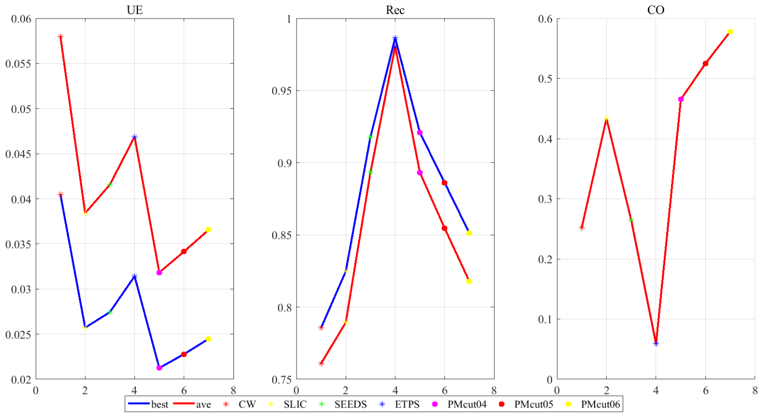
UE. Top $2$ rows of Fig. 4 plots the UE score of each method against the increasing number of superpixels. The first row depicts results on the $100$ images with $S\&P$ noise, and the second row another $100$ images with Gaussian noise. PMcut is the clear winner on UE score with SLIC comes next place, while CW is the clear loser. There is a clear tread that with increasing number of superpixels, UE score gets better.

Rec. Rec score of each method is plotted similarly in the bottom $2$ rows of Fig. 4. On both kinds of noisy images, we can easily identify ETPS is the top performing method. SEEDS and PMcut come the next places, while there is no clear loser. There is also a tread that with increasing number of superpixels, REC score gets better, with the exception on SEEDS.

CO. Fig. 5 shows the CO score. In comparison with other algorithms, PMcut shows a significant advantage, and ETPS has the worst score. While ETPS has the best Rec score, this again demonstrates the trade-off between Rec and CO.

OP. Since all the competing algorithms are trained towards OP, it is thus the most important score in this paper. We report that PMcut achieves the $1st$ place on all $24$ scenarios. We depict one table of OP scores that contains $1$ (out of $2$) noise type, $1$ (out of $4$) superpixel size and $3$ ways of computing score in the supplementary materials. Table 1 shows the average OP score amongst all.

Time. While all the other superpixel algorithm takes less than $1$ second, the run time of PMcuts is doomed by the $\mathcal{NP}$-hard nature of the MILP. Among all, CW and PB are the fastest, on average take only $0.01$ sec.

We set a time limit of each rectangular patch of PMcut to be $2$, $0.5$, $0.1$ and $0.05$ sec, for the desired superpixel size (also the number of MILPs) of $600$, $1200$, $1800$ and $2400$ respectively. The corresponding total average running time for the whole image is $272$, $134$, $40$ and $27$ secs. Finally, the average Gurobi MIP gap is $12.2\%$, $9.8\%$, $10.3\%$ and $9.8\%$, respectively.

One can imagine that as the number of rectangular patches increases, the total time as well as the average MIP gap would decrease. In addition, parallelism can be fully adopted to speed up computation.

Visual quality can be determined by considering compactness, regularity and smoothness. Here, regularity corresponds to both the size and the arrangement of each superpixel, and smoothness refers to the superpixel’s boundary. Fig. 6 shows superpixel results on $3$ images (with two kinds of noises) using all methods, with approximate superpixel number equals $600$ and $1200$. Note that these images are intended to be representative, but superpixel segmentations may vary across different images.

Most of the algorithms provide solid adherence to salient image boundaries, especially when the number of superpixels is large. Compactness and smoothness vary a lot across algorithms and a compactness parameter is beneficial to control the degree of compactness which allows to trade boundary adherence for CO. Ideally, compactness should be increased while only slightly sacrificing Rec.

At a first glance, the superpixels generated by PMcut, SLIC are visually more appealing. Superpixels of PMcut are initialized and bounded by each rectangular patch. Since most of them consist of only background, the resulting superpixel fill in the whole rectangular patch. Hence most of the superpixels are compact and regular in size. PMcut also benefits from the penalty term $\lambda$ on the boundary length, thus creating smooth superpixels. It happens that SLIC loses track of some boundary details, e.g., the helmet in the third image.

In contrast, although being able to capture most of the important boundaries (with high Rec), ETPS and SEEDS produce highly irregular and non-smooth superpixels. Their superpixel size varies a lot, with many tiny superpixels and yet huge ones. One can hardly recognize the original image, if the number of superpixel is large, e.g., ETPS in the second image.

In conclusion, we find that the evaluated ETPS and SEEDS show inferior visual quality. On the other hand, PMcut and SLIC demonstrate good visual quality at the expense of missing several boundaries. Overall, PMcut and SLIC achieve good balance between accuracy and visual appearance.

We conduct additional experiments by first applying [21] (we set the two parameters $\sigma_{s}=5$ and $h=0.55\sigma_{n}$, where $\sigma_{n}$ is the noise variance of $n$ pixels.) to denoise the $100$ images with Gaussian noise. The competing superpixel algorithms are then run on the $100$ denoised images, then being compared to PMcut directly applied to the noisy images. The result is shown in Fig. 7 against on the noisy images, where $\#=1200$ and only the best of $5$ ground-truth score is depicted. As one can notice, all algorithms actually performs worse on the Rec score, while better on the CO score. We think it may be due to the fact that the denoising algorithm smooths the boundary too much. The average running time for the sophisticated denoising algorithm is over $60$ secs per image, hence our running time is superior in this case.

Finally, we conduct experiments on adopting different values of regularization parameter $\sigma$ ($0.4$, $0.5$ and $0.6$) and time limit ($0.05$, $0.1$ and $0.15$ secs) within each patch of the image. Fig. 8 shows two experiments on images with two kinds of noises. It is obvious that when the regularization parameter $\sigma$ grows, Rec and UE become worse while CO better. Also, when the time limit increases, all three scores benefits, thus a trade-off between time and scores. We also report that the average MIP gap of adopting the $3$ time limits are $12.8\%$, $10.3\%$ and $9.5\%$.

References

- [1] Ren, X., Malik, J.: Learning a classification model for segmentation. International Conference on Computer Vision 1 (2003) 10–17
- [2] Achanta, R., Shaji, A., Smith, K., Lucchi, A., Fua, P., Susstrunk, S.: Slic superpixels compared to state-of-the-art superpixel methods. IEEE Transactions on Pattern Analysis and Machine Intelligence 34(11) (2012) 2274–2282
- [3] Stutz, D., Hermans, A., Leibe, B.: Superpixels: an evaluation of the state-of-the-art. Computer Vision and Image Understanding (2017) 1–32
- [4] Felzenszwalb, P.F., Huttenlocher, D.P.: Efficient graph-based image segmentation. International Journal of Computer Vision 59(2) (2004) 167–181
- [5] Shi, J., Malik, J.: Normalized cuts and image segmentation. IEEE Transactions on Pattern Analysis and Machine Intelligence 22(8) (2000) 888–905
- [6] Neubert, P., Protzel, P.: Compact watershed and preemptive slic: on improving trade-offs of superpixel segmentation algorithms. The 22nd International Conference on Pattern Recognition (2014) 996–1001
- [7] Meyer, F.: Color image segmentation. 1992 International Conference on Image Processing and its Applications (1992) 303–306
- [8] den Bergh, M.V., Boix, X., Roig, G., de Capitani, B., Gool, L.V.: Seeds: Superpixels extracted via energy-driven sampling. European Conference on Computer Vision (ECCV) (2012) 13–26
- [9] Yao, J., Boben, M., Fidler, S., Urtasun, R.: Real-time coarse-to-fine topologically preserving segmentation. IEEE Conference on Computer Vision and Pattern Recognition (CVPR) (2015) 2947–2955
- [10] Potts, R.B., Domb, C.: Some generalized order-disorder transformations. Proceedings of the Cambridge Philosophical Society 48 (1952) 106–109
- [11] Nguyen, R.M.H., Brown, M.S.: Fast and effective l0 gradient minimization by region fusion. International Conference on Computer Vision (2015) 208–216
- [12] Bertsimas, D., King, A., Mazumder, R.: Best subset selection via a modern optimization lens. The Annals of Statistics 44(2) (2016) 813–852
- [13] Andres, B., Kappes, J.H., Beier, T., Köthe, U., Hamprecht, F.A.: Probabilistic image segmentation with closedness constraints. International Conference on Computer Vision (2011) 2611–2618
- [14] Kappes, J.H., Speth, M., Andres, B., Reinelt, G., Schnörr, C.: Globally optimal image partitioning by multicuts. International Workshop on Energy Minimization Methods in Computer Vision and Pattern Recognition (2011) 31–44
- [15] Sontag, D., Choe, D., Li, Y.: Efficiently searching for frustrated cycles in map inference. In: Proceedings of the Twenty-Eighth Conference on Uncertainty in Artificial Intelligence. UAI’12, Arlington, Virginia, United States, AUAI Press (2012) 795–804
- [16] Johnson, J.: Convex Relaxation Methods for Graphical Models: Lagrangian and Maximum Entropy Approaches. PhD thesis, Cambridge, MA, USA (2008) AAI0821536.
- [17] Batra, D., S.Nowozin, P.Kohli: Tighter relaxations for map-mrf inference: A local primal-dual gap based separation algorithm. (November 2011)
- [18] Levinkov, E., Uhrig, J., Tang, S., Omran, M., Insafutdinov, E., Kirillov, A., Rother, C., Brox, T., Schiele, B., Andres, B.: Joint graph decomposition & node labeling: Problem, algorithms, applications. In: IEEE Conference on Computer Vision and Pattern Recognition (CVPR). (2017)
- [19] Storath, M., Weinmann, A.: Fast partitioning of vector-valued images. SIAM Journal on Imaging Sciences 7(3) (2014) 1826–1852
- [20] Schick, A., Fischer, M., Stiefelhagen, R.: Measuring and evaluating the compactness of superpixels. The 21st International Conference on Pattern Recognition (ICPR) 2 (2012) 930–934
- [21] Buades, A., Coll, B., Morel, J.M.: A non-local algorithm for image denoising. In: CVPR. (2005) 60–65
5 Appendix
5.1 Proof for Theorem
5.2 Proof for Theorem
Proof.
We prove this by stating that every satisfies the multicut constraints (a).
5.3 Proof for Theorem
Let be the set of all feasible solutions to the corresponding multicut problem (4) with respect to the Potts (3). Since the chordless multicut constraints (a) are facet-defining for the multicut polytope (convex hull of ), we just need to prove .
From Theorem , we know . We prove as follows. For any feasible solution of (4), it naturally defines a valid segmentation in the Potts model (3). We can then compute the corresponding by by fitting a linear function within each segment. Thus, we have constructed a feasible solution , which in turn implies the existence of . ∎