Optimizing Sponsored Search Ranking Strategy by Deep Reinforcement Learning
Abstract.
Sponsored search is an indispensable business model and a major revenue contributor of almost all the search engines. From the advertisers’ side, participating in ranking the search results by paying for the sponsored search advertisement to attract more awareness and purchase facilitates their commercial goal. From the users’ side, presenting personalized advertisement reflecting their propensity would make their online search experience more satisfactory. Sponsored search platforms rank the advertisements by a ranking function to determine the list of advertisements to show and the charging price for the advertisers. Hence, it is crucial to find a good ranking function which can simultaneously satisfy the platform, the users and the advertisers. Moreover, advertisements showing positions under different queries from different users may associate with advertisement candidates of different bid price distributions and click probability distributions, which requires the ranking functions to be optimized adaptively to the traffic characteristics. In this work, we proposed a generic framework to optimize the ranking functions by deep reinforcement learning methods. The framework is composed of two parts: an offline learning part which initializes the ranking functions by learning from a simulated advertising environment, allowing adequate exploration of the ranking function parameter space without hurting the performance of the commercial platform. An online learning part which further optimizes the ranking functions by adapting to the online data distribution. Experimental results on a large-scale sponsored search platform confirm the effectiveness of the proposed method.
Keywords:
Sponsored search, ranking strategy, reinforcement learning1. Introduction
Sponsored search is a multi-billion dollar business model which has been widely used in the industrial area (Haibin and Cantu-Paz, 2010; Chakrabarti et al., 2008). In the commonly employed pay-per-click model, advertisers are charged for users’ clicks on their advertisements. The sponsored search platform ranks the advertisements by a ranking function and select the top ranked ones to present to the users. The price charged from the advertisers of these presented advertisements is computed by the generalized second price (GSP) auction mechanism (Edelman et al., 2007; Myerson, 1981) as the smallest price which is sufficient to maintain their allocated advertisement showing positions. Traditionally, the ranking score of an advertisement is set to be its expected revenue to the sponsored search platform, computed as the product between the advertisers bid price and the predicted click-through rate (CTR) of the user.
The expected revenue based ranking function dominates the sponsored search area, and most of the existing methods focus on designing elaborate models to predict the CTR (Yu et al., 2012; Li et al., 2010; Haibin and Cantu-Paz, 2010; McMahan et al., 2013). In this work, instead of designing a CTR prediction model, we try an alternative way to add more flexibility in the ranking function for balancing the gain between users, advertisers and our advertisement platform. For the user experience, we recognize the engagement of users as their CTR on the advertisements and a term is added to the ranking function which are monotonic of the users’ CTR. To improve the advertisers’ return on their spending, we add a term related to the users’ expected purchase amount. The ranking function is then computed as the weighted sum of the two terms together with the expected revenue term.
Although the ranking function can well represent the benefits of the platform, user and advertisers, it may not be directly related to the benefits of these players. First of all, owing to the second price auction mechanism (Edelman et al., 2007), the advertisers are charged by the minimum amount of dollars they need to keep their advertisement position, not the amount of money they bid. The price is determined by the competitiveness of the underlying advertisement candidates. Second, the CTR and CVR (i.e., conversion rate, the ratio of buying behavior after each advertisement click) are predicted by a prediction model, which is generally biased and prone to noise because of being training on a biased distributed dataset (Joachims et al., 2017). To link the real world benefits of the users, advertisers and platform directly to the ranking function, we propose a reinforcement learning framework to learn the ranking functions based on the observed gain in a ‘trail-and-error’ manner. By treating the ranking function parameter tuning as a machine learning problem, we are able to deal with more complex problems including higher parameter space and traffic characteristic based tuning. Advertisement showing positions associated with different queries and different users exhibit diverse characteristics in terms of distribution of bid price and CTR/CVR. Tuning the parameters according to traffic characteristics would definitely improve the performance of the ranking function.
The reinforcement learning (Sutton and Barto, 1998) is generally used in sequential decision making, which follows an explore and exploit strategy to optimize the control functions of the agents. Starting from its proposal, it is mostly used in games and robotics applications (Mnih et al., 2015; Silver et al., [n. d.]; Li, 2017) where the exploration can be done in a simulated or artificial environment. When utilizing the algorithms in advertising platforms, we need to consider the cost for the exploration and try to perform exploration in a simulated environment. However, different from the games, simulating the advertisement serving and rewards (click, user purchase, etc.) is hard due to the large space of controlling factors like user intention, traffic distribution changes, advertisers budget limitation etc. In this work, we build a simulated sponsored search environment by making the historical advertisement serving replayable. Specifically, the simulated environment is composed of an advertisement replay dataset (state in the terminology of reinforcement learning), which for each advertisement showing chance, stores the full list of advertisement candidates together with their predicted CTR, CVR and the advertisers’ bidding prices, and a set of ‘virtual’ exploration agents which simulate the advertisement results and users’ response under different ranking functions (i.e., actions in reinforcement learning terminology). The reward for the exploration is computed by reward shaping methods (Ng et al., 1999).
However, there are two problems with the simulated environment: (1) the simulated state-action-reward tuple is temporally independent: it is hard to simulate the temporal correlation between the response of a user on one advertisement and the response on the next presented advertisement; (2) the simulated response is inconsistent with online user response to some extent. To solve problem (1), we employ an off-policy reinforcement learning architecture (Lillicrap et al., 2015) to optimize the advertisement ranking function, which does not require the observation of the next states’ action and reward. For problem (2), we use an offline calibration method to adjust the simulated rewards according to the online observed reward. Moreover, after the offline reinforcement learning, we employ an online learning module to further tune the reinforcement learning model to better fit the real-time market dynamics.
Contributions. In this work, we present our work of optimizing the advertisement ranking functions on a popular mobile sponsored search platform. The platform shows the search results to users in a streaming fashion, and the advertisements are plugged in fixed positions within the streaming contents. Our main contributions are summarized as follows:
- •
We introduce a new advertisement ranking strategy which involves more business factors like the user engagement and advertiser return, and a reinforcement learning framework to optimize the parameters of the new ranking function;
- •
We propose to initialize the ranking function by conducting reinforcement learning in a simulated sponsored search environment. In this way, the reinforcement learning can explore adequately without hurting the performance of the commercial platform;
- •
We further present an online learning module to optimize the ranking function adaptively to online data distribution.
2. Related Works
Auction mechanisms have been widely used in Internet companies like Google, Yahoo (Edelman et al., 2007) and Facebook (Vickrey, 1961) to allocate the advertisement showing positions for the advertisers. The Internet advertising auction generally works in the following procedure: an advertiser submit a bid price stating their willingness to pay for an advertisement response (click for a performance-based campaign, view for a branding campaign, etc.) The publisher ranks the advertisements according to their quality scores and bid prices, and presents the top ranked ones to the users together with the organic contents. The advertisers are then charged, for the response of the users, the minimum amount of dollars to keep the showing positions of their advertisements. The auction mechanism has been extensively studied in the literature both theoretically and empirically: Bejamin et al. in (Edelman et al., 2007) investigate the properties of generalized second price (GSP) and compare it with the VCG (Vickrey, 1961) mechanism in terms of the equilibrium behavior. In (Mehta et al., 2007), the authors formulate the advertisement allocation problem as a matching problem with budget constraints, and provide theoretical proof that the algorithm can achieve a higher competitive ratio than the greedy algorithm. To solve the ineffectiveness in next-price auction, the authors in (Aggarwal et al., 2006) designs a truth-telling keyword auction mechanism. In (Myerson, 1981) followed by (Edelman and Schwarz, 2010), the reserved price problem is studied, including its welfare effects and its relation to equilibrium selection criteria. A field analysis on setting reserve prices in sponsored search platforms of Internet companies is presented in (Ostrovsky and Schwarz, 2011). Existing work generally focuses on the revenue effect of the auction mechanism to make it efficient in the bidding process and capable of profiting more revenue. In our work, we use the generalized second price (GSP) auction for pricing. But since we are working on an industrial sponsored search platform, in consideration of long term return, instead of maximizing the platform revenue only, we also add the user experience and advertiser utility terms into the ranking function.
Reinforcement learning problem is basically modeled as a Markov Decision Process (Sutton and Barto, 1998), which concerns with how agents adjust their policy to interact with the environment so as to maximize certain cumulative rewards. Recently, with the combination of deep neural network (LeCun et al., 2015), the reinforcement learning methods are able to work in the environment with high-dimensional observations by feeding large-scale experience data and training with powerful computational machines (Li, 2017), and make breakthrough in many different areas including game of Go (Silver et al., [n. d.]), video games (Wu and Tian, 2017; Mnih et al., 2016), natural language processing systems (Wu et al., 2016; Su et al., 2016) and robotics (Schulman et al., 2015; Levine et al., 2016). However, most of the existing applications are conducted on simulated non-profitable platforms, where the experience data are easy to acquire and there is no restrict to try any agent policies and training schemes. In a commercial system, however, the exploration of the reinforcement learning may bring in uncertainty in the platform’s behavior, prone to loss of revenue, thus offline methods are a practical solution (Zhang et al., 2016). In (Li et al., 2016), Li and Lipton et al. design a user simulator under movie booking scenario. The simulator is designed on some rules and data observations. However, in our platform, there are far more factors (users, advertisers) to simulate. For online advertising with reinforcement learning, the authors in (Amin et al., 2012) first propose to tune sponsored search keyword bid price in an MDP framework, where the state space is represented by the auction information, the advertisement campaign’s remaining budgets and life-time, while the actions refer to the bid price to set. Then in (Cai et al., 2017), the authors formulate the sequential bid decision making process in the real-time bidding display advertising as a reinforcement learning problem. The method is based on assumptions that the winning rate depends only on the bid price and the actual clicks can be well estimated by the predicted CTR. Hence, enabling the best bidding strategy can be computed in an offline fashion. In our work, we initialize the reinforcement learning model using the offline simulated data, and combine the reward shaping method and online model update procedure to make the model consistent with the online data distribution.
3. System Overview
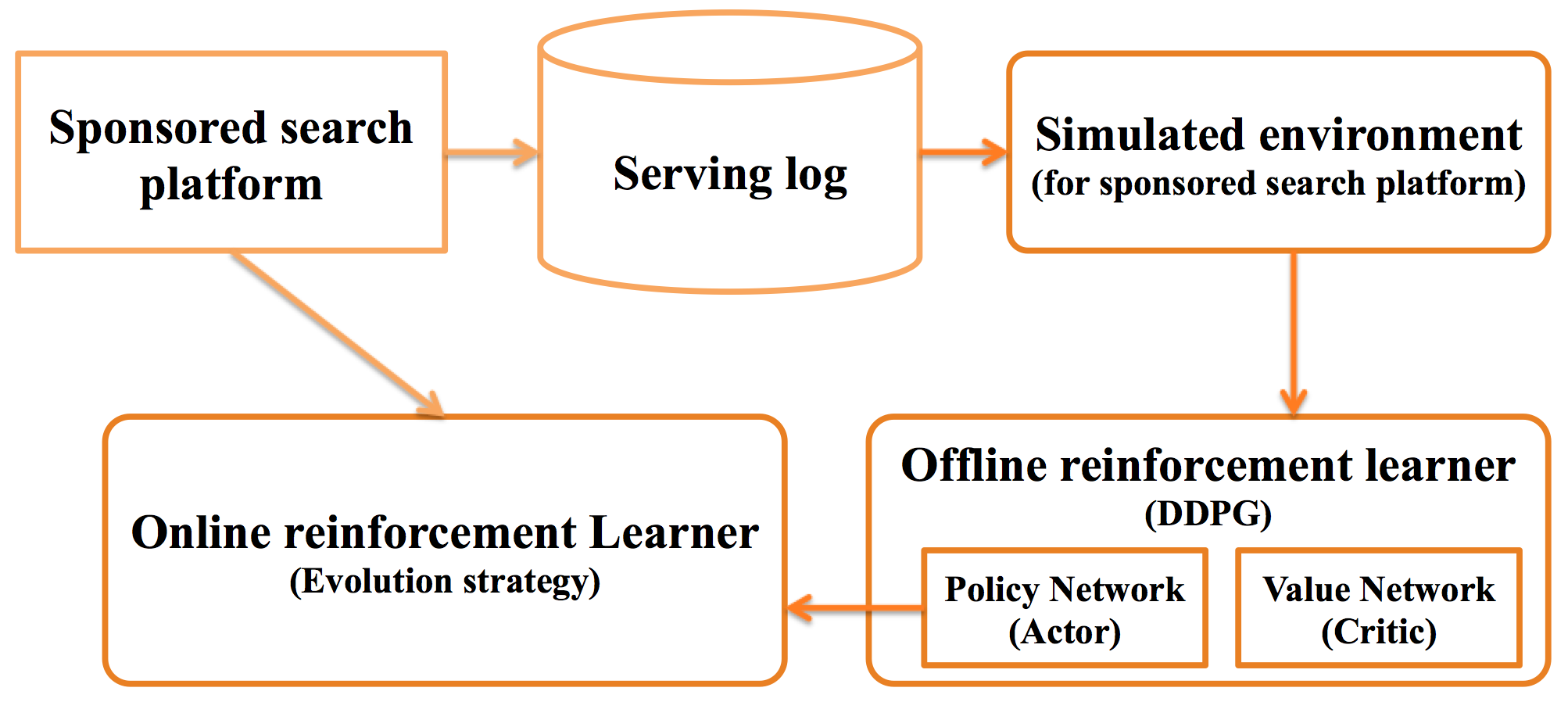
As shown in Fig. 1 (highlighted in orange), the whole system is composed of three modules: the offline sponsored search environment simulation module, the offline reinforcement learning module and the online reinforcement learning module. The environment simulation module is used to simulate the effect caused by changing the ranking function parameters, including re-ranking the advertisement candidates, showing the new top-ranked advertisement, and generating the users’ response with respect to such changes. To allow adequate exploration, the offline reinforcement learning module collects training data by deploying randomly generated ranking functions on the simulated environment. An actor-critic deep reinforcement learner (Lillicrap et al., 2015) is then trained on top of these training data. To bridge the gap between the offline simulated data and the online user-advertiser-platform interaction, we build an online learning module to update the model by the online serving results.
3.1. Ranking Strategy Formulation
We use the following ranking function to compute the rank score for advertisement
| (1) |
where represents the search context including the search query, user demographic information and status of advertisement candidates for the advertisement showing chance. and are the bid price and product price set by the advertiser for the advertisement on the current query. and of are predicted by the platform. performs nonlinear monotonic projection on and , and scalar are used to balance the weights between the three terms. Because our sponsored search platform charges the advertisers by ‘click’, the first term can be seen as the expected revenue of the platform. We refer the users’ preference to the presented advertisements as their response ratio (CTR and CVR). Hence, the second term indicates the engagement of the users. The third term computes the expected return (expected user purchase amount) of the advertiser by showing the advertisement, which measures the gain of the advertisers. According to the GSP rule, if the advertisement is shown, its advertiser is charged
| (2) |
where is the advertisement just ranked below . However, there is possibility that the numerator is a negative value. In our implementation, we solve this problem by imposing a lower bound on the , just like the reserve price (Ostrovsky and Schwarz, 2011), and since the platform revenue is always one of the optimization goal, the numerator is rarely negative in the experiments. Compared with the ranking function proposed in (Lahaie and McAfee, 2011), which is generally used by Google and Yahoo, our ranking function (1) involves more parameters and commercial factors to consider, which can be used to optimize for more comprehensive commercial goals.
The ranking function is parameterized by in consideration of the following issues: first, the predicted CTR and CVR are generally biased due to the imbalance training data, and need to be calibrated to make it consistent with the online user response; second, we charge the advertisers according to second price auction mechanism, which is lower than the bid price and computed according to the next ranked advertisement; third, the three terms may not be the same in numeric scale. The ranking function optimization problem can be formulated as to predict the best parameter given the search context as
| (3) |
where is the reward given the ranking function . The reward can be defined as the sum of purchase amount, number of click and platform revenue or any weighted combinations of the three terms during a certain period after the ranking function is operated, depending on the platform performance goal. Since in the reinforcement literature, is used to represent the action of the learning agent, we take this notation to align with the literature.
3.2. Long-term Reward Oriented Ranking Function Optimization
Reinforcement learning methods are designed to solve the sequential decision making problem, in order to maximize a cumulative reward. In the literature, it is generally formulated as optimizing a Markov decision process (MDP) which is composed of: a state space , an action space , a reward space with a reward function and a stationary transition dynamic distribution with conditional density which satisfies Markov property for any state-action transition process . The action decision is made through a policy function parameterized by . The reinforcement learning agent interacts with the environment according to giving rise to a state-action transition process , and the goal of the learning agent is to find a which maximizes the expected discounted cumulative reward where and represents the initial state distribution.
The ranking function learning of a sponsored search platform has many special characteristics making it suitable to be formulated under the reinforcement learning framework. First of all, during one user-search session, the sponsored search platform sequentially makes decisions on choosing ranking functions to presenting advertisements for the user. Second, during the interaction with users, the platform collects users’ response as rewards and balances between the exploration and exploitation to maximize the long term cumulative rewards. Third, since the data distribution chances during the time, it requires online learning for adaptation. In this work, we choose the reinforcement learning methodology to learn the ranking function in Eq. (3) for continuously improving the long term rewards. Specifically, in our scenario, the state is defined as the search context of a user query including the query terms, query categories, user demographic information and online behavior. The sponsored search platform (i.e., reinforcement learning agent in our scenario) uses the ranking function as an action to rank the advertisements and interacts with a user to get the reward as the combination of platform revenue, user engagement (quantified as user click, purchase, etc.) and advertiser’s sale amount. Then the environment transits to the next state . The reinforcement learning method optimizes the ranking function parameters through exploring and exploiting on the observed state-action-reward-state tuples.
4. Method
In the following sections, we will introduce the detail algorithms of the three modules in Fig. 1.
4.1. Environment Simulation Module
On one hand, the performance of the reinforcement learning is guaranteed by adequate exploration; on the other hand, the exploration may bring uncertainty in the ranking functions’ behavior and have performance cost. Since the algorithm is designed to run on a commercial sponsored search platform, we minimize the exploration cost by building a simulated sponsored search environment to training the reinforcement learning model in an offline manner.
The sponsored search procedure is effected by many factors including the advertisers’ budgets and bidding prices, the users’ propensity and intention, making the procedure hard to simulate from scratch. In this work, instead of generating the whole sponsored search procedure, we propose to do the simulation by replaying the existing advertisement serving processes and make them adjustable in terms of ranking function setting. Given a user query, the platform proceeds by retrieving a big set of advertisements according to semantic matching criterion, predicting the CTR and CVR for these advertisements, and computing the rank scores of them for advertisement selection and click price estimation. To make the advertisement ranking process replayable, for each advertisement showing chance, we store the bidding information and predicted CTR, CVR of all the associated advertisement candidates. According to Eqs.( 1) and (2), the ranking orders and click prices for these advertisement candidates can be computed out of these replay information. The reward for showing an advertisement is simulated by the reward shaping approach (Ng et al., 1999) as the user response (like clicking the advertisement or purchasing the product). For example, if our goal is to get more platform revenue and user clicks, the intermediate reward can be computed as
| (4) |
where is a manually tunable parameter to balance between the expectation of more user engagement (click behavior) or more platform revenue. To the best of our knowledge, most of the prediction algorithms concentrate on ordering the response rate of the advertisement instead of predicting the true value, and are trained on the biased data (Joachims et al., 2017). As a result, there is a gap between the ground truth user response rates and the predict ones. To guarantee the reinforcement learning method optimize towards the right direction, we minimize the gap by CTR and CVR calibration.
4.1.1. Reward Calibration

In Fig. 2, we illustrate the difference between the predicted CTR and groundtruth CTR on different device types and different advertisement showing positions. The advertisement showing chances (impressions) are grouped into bins by discretizing their predicted CTR values, and the groundtruth CTR of a bin is computed as the number of clicks achieved by the impressions in this bin divided by the number of impressions. It can be seen that, the predicted CTR and the groundtruth CTR exhibit diverse mapping relations on different context (e.g. device type, location). We manually select some context features which effect the mapping relations most, and calibrate the predicted CTR as
| (5) |
where refers to the manually selected feature fields like time and device type, is the averaged ground truth CTR. To maintain the ordering relations of the predicted CTR on the set of advertisements, we employ the Isotonic regression method (Best and Chakravarti, 1990) to compute the calibrated values for each combinations. The method can automatically divide the CTR values into bins, targeting at minimizing the least square error between the predicted CTRs and the calibrated ones. By grouping the advertisement showing results into bins according to the binned CTR values, the ground truth for a bin is computed as the number of observed clicks in this bin divided by the number of presented advertisements. CVR is calibrated in the same way.
4.2. Offline Reinforcement Learning for Ranking Function Initialization
In this section, we will introduce the reinforcement learning problem formulation, the model architecture and the training method based on the simulated environment introduced above. Regarding to the MDP representation in Section 3.2, for each advertisement showing chance, we define the state as the search context composed of three types of features: (1) query related features like query ID, query category ID; (2) user demographic and behavior features including age, gender and aggregated click number on certain advertisement; (3) advertisement related features, e.g. advertisement position. The action is the ranking function parameter vector in Eq. (1), and reward is defined as Eq. (4). Since user intention is difficult to model correctly, it is hard to predict whether a user would switch to another specific query after seeing current advertisement. Thus we focus on the state transitions in each search session and omit the inter-session ones. To generate the next state , we make simplification by assuming there is no change in query related features. The user behavior features are updated by adding the expected behavior calculated out of the predicted CTR and CVR with calibration (refer to Section 4.1.1). For the advertisement related features, we assume the user are continuously reading the streaming contents and advertisements one by one, and the advertisement related features are updated accordingly.
Learning from the simulated environment introduced above gives rise to many special requirements for the learning algorithm. First of all, the simulation method above could only generate temporally independent state-action pairs, while lacking the capability of simulating the interaction between search sessions. This is because the state-action sequence of user-platform interaction is tangled. The current user behavior is correlated with the previously presented advertisements and occurred user responses. The temporal independency of the training data requires the reinforcement learning method to support off-policy learning (Degris et al., 2012). Second, because the action space is continuous (refer to Eq. (3)), it is practical to define the deterministic policy function (Silver et al., 2014). Moreover, the learning method should be capable of dealing with the complex mapping relation between action and rewards caused by the discontinuously distributed bid price. Taking these requirements into consideration, we use the Deep Deterministic Policy Gradient (DDPG) learning method in (Lillicrap et al., 2015) as the learner to optimize our ranking function. The method supports off-policy learning, and combines the learning power of deep neural networks with the deterministic policy function property in Actor-Critic architecture.
The DDPG algorithm iterates between the value network (critic network) learning step and the policy network (actor network) learning step, the value network estimates the expectation of the discounted cumulative rewards from current time as (an example reward function is shown in Eq. (4))
| (6) |
and the policy network calculates the best ranking function strategy given the current search context as
| (7) |
The parameter and refer to the weights and bias terms in the deep networks.
4.2.1. DDPG Network Architecture
The architectures of the value network and policy networks in our DDPG based reinforcement learning model is shown in Fig. 3. Refer to Eqs. (6) and (7), both the two networks have the current state as input. We represent all the features of (refer to Section 4.2) as ID features, and use a shared embedding layer to convert each of these ID features into a fixed-length dense vector and concatenate them to form the feature representation of . The embedding vectors are initialized as random vectors and updated during the reinforcement learning process. For the policy network, we connect the embedding layer to a fully-connected hidden layer with the Exponential Linear Units (ELU) (Clevert et al., 2015) as activation function. In the experiment, we find that when using activation functions like Sigmoid and ReLU, the output of nodes are easily move to numeric ranges with zero gradients, hindering the propagation of gradients along the network. By employing the ELU as activation function, the networks converge much faster. The hidden layer in the policy network is then concatenated to the output layer by a sigmoid activation function. We also use clip method as (Mnih et al., 2015) to clip the output into a valid range to avoid over-learning.
For the value network, its inputs are composed of the state features () and the action features (ranking function parameter vector ). Different from the state features, the action features are continuous. We connect them each to an independent fully-connected hidden layer with ELU as activation function. The two hidden layers are of the same number of nodes and are connected together to a higher level fully-connected hidden layer. In the output layer, we utilize a dueling network architecture (Wang et al., 2015) which divides the value function () in Eq. (6) into the sum of a state value function () and a state-dependent action advantage function (), such that . According to the insight of (Wang et al., 2015), the dueling architecture makes the learning of the value network efficient by identifying the highly rewarded states and the states where the selected actions do not affect the rewards much. In our work, since our reward is defined on click prices (and product prices), it is highly varied for different states and discontinuous with the change of advertisement candidates ordering. The variance in the rewards poses a big challenge for learning a stable policy function. In our experiments (refer to Section 5.1 and Fig. 6), we observed that the dueling architecture makes the learning process converge more quickly. The observation coincides with the conclusion in (Williams, 1992). Parameter setups of the network will be discussed in experiments.
4.2.2. Learning the Ranking Function from Simulated Environment
We employ the asynchronous training strategy (Nair et al., 2015) to train the DDPG model introduced above. As shown in Fig. 4, the training data is sampled by multiple independent exploration agents. These training agents interact with the simulated sponsored search environment (Section 4.1) by sampling the advertisement serving replay data, trying different ranking functions (actions ’s) on the sampled replay data, and collecting the simulated rewards (Section 4.1.1) and state transitions (Section 4.2) for these actions to build training tuples in the form . The training tuples are then sent to local DDPG reinforcement learners to calculate the gradients of the value network parameters and policy network parameters and update these network parameters individually. The local learners also send their ‘local’ gradients to update the ‘global’ model parameters asynchronously. The algorithm is shown in Algorithm 1. To guarantee the independency and adequate exploration of the local reinforcement learners, we set the exploration agents to act by uniformly sampling from the ranking function parameter space.

In our implementation, we use a distributed computing platform with around 100 GPU machines, and 5 central parameter servers to store the global model parameters. For the distributed computing platform, each process maintains an asynchronous DDPG learner, an exploration agent and a local model (copied from the global model). After several rounds of gradients computation from the simulated training data, the gradients are sent asynchronously to the central parameter servers, and the updated model parameters are sent back to update the local learners’ copies.
4.3. Online Reinforcement Learning for Ranking Function Updating

Despite the effort of reward calibration, the offline simulated environment is still inconsistent with the real online environment due to the dynamic data distribution and sequential correlation between the continuous user behavior. This inconsistency poses the online update requirement for the learned ranking function. However, directly using the asynchronous training framework in Section 4.2.2 is not proper due to the speciality of the online updating: (1) the data distribution is different, where the online rewards are sparse and discrete (e.g. click or non-click, not the click expectation in simulated environment); (2) there are latency in reward collection, for instance, a user clicks an advertisement immediately, but the purchase behavior may be postponed for several days (chapelle2014modeling).
Regarding to these specialities, we introduce the evolution strategy (Salimans et al., 2017) to update the parameters of the policy model. The evolution strategy based online updating method is illustrated in Fig. 5. We perform the following steps to online update the policy networks : (i) stochastically perturb the parameters by a Gaussian noise generator with zero mean and variance . Denote the set of perturbed parameters as . (ii) Hash the the online traffic into bins according to dimensions like user ID and IP address. For each parameter , we deploy a policy network on a traffic bin and get the reward according to Eq. (4) as the weighted sum of platform revenue and the click number in this bin . However, in reality, the number of advertisement showing number should not be exactly the same for each bin. We compute the relative value of the reward by dividing it with the number of served advertisements as . (iii) Update the parameter by the weighted sum of the perturbations as
| (8) |
where is the learning rate. It should be noted that regard to the online stability, we only use a small percentage of traffic (totally 2% of the overall online traffic) for testing the performance of .
The evolution strategy based method has several merits under our scenario. First of all, it is derivative-free. Since the rewards are discrete, it is hard to compute the gradient from the reward to the policy network parameters. Second, by fixing the seed of the random number generator, we just need to communicate the reward (a scalar) between the policy networks in local traffic bins and the central parameter servers. Thirdly, the method does not have intermediate reward requirement due to the homogeneity of these online traffic bins. Thus it can be deployed to optimize conversion related performance.
5. Experimental Results
We conduct experiments on a popular commercial mobile sponsored search platform which serves hundreds of millions of active users monthly covering a wide range of search categories. To fully study the effectiveness of the proposed ranking function learning method, both analytical experiments on offline data and empirical experiments by deploying the learned ranking functions online are carried out. On the platform, the search results are presented in a streaming fashion, and the advertisements are allowed to be shown on fixed positions within the streamed content. Since the search results are tangled with the advertisements, besides the platform revenue, one important issue we need to deal with is the user experience. In the experiments, we design the immediate reward as
| (9) |
where is the amount we charge the advertisers according to generalized second price auction, and is a binary number indicating whether the advertisement is clicked (1) or not (0). is manually set according to the average to balance between the platform revenue goal and the user experience goal. We can also add the advertisers’ satisfactory term like purchase price. But because we test our model on a small percentage of traffic online (2% traffic), the purchase amount is highly varied according to our observation. In the current experiments, we do not show the purchase optimized results and leave it as a future work when we ramp up our test traffic amount.
5.1. Experiments on Offline Data
Since we are learning on a biased sampled data, the mapping relation between the reward and ranking function parameters is complex due to the highly varied distribution of bidding price. The convergence property of the proposed method is worthy of studying. In the offline experiments, we study the convergence property of the proposed method and the effect of using different architectures and different super parameters on the speed of convergence. We employ an analytical method to verify whether the proposed method can converge to the ‘right’ ranking function. In the experiment, a simple state representation (only query + advertisement position) is utilized such that from the simulated data, it is computational feasible to perform brute force search to find the best parameters of the ranking function (refer to Eq. (1)). The brute force method proceeds by uniformly sampling the parameters in at a fixed step size for each replay sample, computing the rewards (refer Eq. (9)) based on the method in Section 4.2.2, and finding the best parameter from these samples according to the aggregated rewards. For training the reinforcement learning model, we encode both the query IDs and advertisement position IDs into 8-dimension embedding vectors. As a result, our embedding layer consists of a 16-dimension feature vector. For the critic hidden layer, we utilize two full-connection units, each of which has 500 nodes, and ELU (Clevert et al., 2015) as the activation function. We use the same settings for the actor hidden layer except using 100 nodes in each layer. The learning rate for network parameter, target network parameter and regularization loss penalty factor are set to be 1.0e-5, 0.01 and 1.0e-5 respectively. The is set to be the average of the calculated out of the data log. Experimental results are presented in Fig. 6. The performance of the proposed method is measured by the squared error between the learnt ranking function parameters and the ‘best’ parameters found by brute force method. From the results, we can see, the proposed method could converge gradually to the best ranking function as the training process goes on.
We also evaluate the performance improvement brought by the dueling architecture in Fig. 6. Comparing the results of using the dueling architecture (annotated by ‘dueling’ in the figure) and not (‘without dueling’), it can be seen that, the dueling architecture improve the convergence speed dramatically. The intuition behind the results is the dueling architecture could help remove the reward variance of the same action under different states by , and guide the action-value network to focus more on differentiating between different actions. As a result, the policy network learning is accelerated. In Fig. 7, we evaluate the influences of different super parameters for training the model, including the learning rate, regularization penalties and batch sizes. The parameter setup is listed in Table 1. As can be observed, lower learning rate (‘base’ and ‘learning rate’) makes the learning method converge more smoothly and larger batch size (‘base’ and ‘batch size’) and lower regularization penalty (see ‘base’ and ‘regular’) make the learning method converge more closely to the optimal solution. This is because there is strong variance in the rewards. Lower learning rate and larger batch size helps to reduce the variance in the batched training data, and lower regularization penalty allows a larger searching space for variables.
| ID | Learning rate | Regularization | Batch size |
|---|---|---|---|
| base | 1.0e-5 | 1.0e-5 | 50k |
| learning rate | 1.0e-4 | 1.0e-5 | 50k |
| batch size | 1.0e-5 | 1.0e-5 | 10k |
| regular | 1.0e-5 | 1.0e-3 | 50k |
5.2. Online Serving Experiments
In this section, we present the experimental results of conducting a bucket experiment on a popular sponsored search platform. The sponsored search platform charge the advertisers for the click on their advertisements according to GSP auction mechanism. We split a small percentage (about 2%) of traffic from the whole online traffic by hashing the user IDs, IP addresses, etc., and deploy the learned ranking function online for advertisement selection and pricing. The following business metric are measured to see the improvement brought by the proposed method. (1) Revenue-Per-Mille (RPM): the revenue generated per thousand impressions; (2) Price-Per-Click (PPC): the average price per-click determined by the auction; (3) Click-through-rate (CTR). We employ the three business metrics because we are optimizing towards the platform revenue and user experience as in Eq. (9). RPM is determined by the product of CTR and PPC. From the change of CTR and PPC, we can also induce the improvements of the advertisers’ saling efficiency, i.e. increase in CTR and decrease in PPC means the advertisers can attract more customers by less spending on advertisement serving.
In this work, a new ranking function is proposed by adding the terms reflecting the user engagement and the advertisers’ gain, and a reinforcement learning method is presented for learning the optimal parameter of this term. In the online experiments, we want to verify the performance improvement brought by the new ranking function and the improvement from the reinforcement learning method. To evaluate the effectiveness of the new ranking function, we compare the proposed ranking function with the one proposed by Lahaie and McAfee (Lahaie and McAfee, 2011). The ranking function in (Lahaie and McAfee, 2011) has been employed by many companies and proved to be efficient in online advertising auctions. In the experiment, we use this ranking function as the baseline and set its parameter (the exponential term) by brute force searching in the same manner as Section 5.1. For the proposed method, we use both the ranking functions learned by the brute force method in Section 5.1 and the ranking function learned by the reinforcement learning method. The comparison results on two continuous days’ data are shown in Table 2. As is observed, compared to the method (Lahaie and McAfee, 2011), our ranking function with parameters searched by brute force method is capable of devlivering 2.5% of RPM growth with 1.1% of CTR increase and 1.4% of PPC increase. This observation confirms the effectiveness of the proposed ranking function in improving the platform’s performance. For the ranking function learned by reinforcement learning method, we observe a 2.5% RPM growth which is arisen majorly from the CTR increase (2.0% of CTR gain). We interpret the difference between the reinforcement learning method and ’brute force’ method by the fact that the reinforcement learning method dose not converge to the exact value of brute force method, and it use a more elaborate set of features for learning. From the business side, we can find that the new ranking function can improve more user engagement by attracting more user clickness on the presented advertisements. For the platform, the increase of RPM brings in more efficiency in earn platform profit, and for the advertisers, the RPM growth is driven by the CTR increase while there is a little increase in PPC (for the learned ranking function), this means, the advertisers only need pay a litter more money to attract more potential buyers.
Section 4.3 introduces the online evolution strategy method for tuning the policy networks based on online data. In this experiment, we evaluate the online performance changes in seven continuous days to confirm the performance increases brought by online learning method. To disturb strategy actions in , we add a gaussian noise with mean 0 and variance to the parameters of . We split the traffic of the test bucket into a number of splits and apply each perturbed policy networks to one of them. The buckets and the user feedback history are collected from the data logs to compute the updates in Eq. (8). The average performance of the test bucket are shown in Fig. 8. As can be seen, all the three business metrics improves during the days. Compared with the baseline ranking function (Lahaie and McAfee, 2011) (whose parameter stay unchanged during the days), the RPM grows from 2% to 4%, CTR grows from 2% to about 3%. The results indicate the effectiveness of the online updating method. We also find the PPC grows because there is no constraints added on it. In the future work, we will try to add constraints to limit PPC increase to generate more return for advertisers.
| Metrics (%) | |||
|---|---|---|---|
| McAfee (Lahaie and McAfee, 2011) | 0.00 | 0.00 | 0.00 |
| brute force | 2.55 | 1.12 | 1.45 |
| offline learning | 2.52 | 2.08 | 0.26 |
6. Conclusions
It is commonly accepted when building a commercial sponsored search platform, besides the intermediate platform revenue, the users’ engagement and the advertisers’ return are also important to the long-term profit of the commercial platform. In this work, we design a new ranking function by incorporating these factors together. However, these additional terms increase the complexity of the ranking function. In this work, we propose a reinforcement learning framework to optimize the ranking function towards the optimal long-term profit of the platform. As is known, the reinforcement learning works in a trail-and-error manner. To allow adequate exploration without hurting the performance of the commercial platform, we propose to initialize the ranking function by an offline learning procedure conducted in a simulated sponsored search environment, followed by an online learning module which updates the model adaptively to online data distribution. Experimental results confirms the effectiveness of the proposed method.
In the future, we will focus on the following directions: (1) Sequential user behavior simulation. The environment simulation method introduced in Section 4.1 is limited to one time advertisement serving without considering the correlation between sequential user behaviors. We plan to try generative models like GAN (Goodfellow et al., 2014) to model the continuous user behaviors. (2) The proposed method has the ability to improve advertisers’ return-per-cost by adding the purchase amount into the reward term. Due to traffic limitation, we did not investigate on this effect, in future work, we will increase the online testing traffic to measure the gain brought by adding the purchase amount reward.
References
- Aggarwal et al. (2006) Gagan Aggarwal, Ashish Goel, and Rajeev Motwani. 2006. Truthful auctions for pricing search keywords. In Proceedings of the 7th ACM conference on Electronic commerce.
- Amin et al. (2012) Kareem Amin, Michael Kearns, Peter Key, and Anton Schwaighofer. 2012. Budget optimization for sponsored search: Censored learning in MDPs. UAI (2012).
- Best and Chakravarti (1990) Michael Best and Nilotpal Chakravarti. 1990. Active set algorithms for isotonic regression: a unifying framework. Mathematical Programming 1–3 (1990), 425–429.
- Cai et al. (2017) Han Cai, Kan Ren, Weinan Zhang, Kleanthis Malialis, Jun Wang, Yong Yu, and Defeng Guo. 2017. Real-Time Bidding by Reinforcement Learning in Display Advertising. In Proceedings of the ACM International Conference on Web Search and Data Mining. 661–670.
- Chakrabarti et al. (2008) Deepayan Chakrabarti, Deepak Agarwal, and Vanja Josifovski. 2008. Contextual advertising by combining relevance with click feedback. In Proceedings of the International Conference on World Wide Web. 417–426.
- Clevert et al. (2015) Djork-Arné Clevert, Thomas Unterthiner, and Sepp Hochreiter. 2015. Fast and Accurate Deep Network Learning by Exponential Linear Units (ELUs). Computer Science (2015).
- Degris et al. (2012) Thomas Degris, Martha White, and Richard Sutton. 2012. Off-Policy Actor-Critic. In Proceedings of International Conference on Machine Learning.
- Edelman et al. (2007) Benjamin Edelman, Michael Ostrovsky, and Michael Schwarz. 2007. Internet Advertising and the Generalized Second-Price Auction: Selling Billions of Dollars Worth of Keywords. American Economic Review 97, 1 (2007), 242–259.
- Edelman and Schwarz (2010) Benjamin Edelman and Michael Schwarz. 2010. Optimal auction design and equilibrium selection in sponsored search auctions. The American Economic Review 100, 2 (2010), 597–602.
- Goodfellow et al. (2014) Ian Goodfellow, Jean Pouget-Abadie, Mehdi Mirza, Bing Xu, David Warde-Farley, Sherjil Ozair, Aaron Courville, and Yoshua Bengio. 2014. Generative adversarial nets. In Proceedings of Advances in Neural Information Processing Systems. 2672–2680.
- Haibin and Cantu-Paz (2010) Cheng Haibin and Erick Cantu-Paz. 2010. Personalized click prediction in sponsored search. In Proceedings of the ACM International Conference on Web Search and Data Mining.
- Joachims et al. (2017) Thorsten Joachims, Adith Swaminathan, and Tobias Schnabel. 2017. Unbiased learning-to-rank with biased feedback. In Proceedings of the ACM International Conference on Web Search and Data Mining.
- Lahaie and McAfee (2011) Sébastien Lahaie and R Preston McAfee. 2011. Efficient Ranking in Sponsored Search. (2011), 254–265.
- LeCun et al. (2015) Yann LeCun, Yoshua Bengio, and Geoffrey Hinton. 2015. Deep learning. Nature 521, 7553 (2015), 436–444.
- Levine et al. (2016) Sergey Levine, Chelsea Finn, Trevor Darrell, and Pieter Abbeel. 2016. End-to-end training of deep visuomotor policies. Journal of Machine Learning Research 17, 39 (2016), 1–40.
- Li et al. (2010) Wei Li, Xuerui Wang, Ruofei Zhang, Ying Cui, Jianchang Mao, and Rong Jin. 2010. Exploitation and exploration in a performance based contextual advertising system. In Proceedings of the ACM SIGKDD International Conference on Knowledge Discovery and Data Mining. 27–36.
- Li et al. (2016) Xiujun Li, Zachary C. Lipton, Bhuwan Dhingra, Lihong Li, Jianfeng Gao, and Yun-Nung Chen. 2016. A user simulator for task-completion dialogues. arXiv preprint arXiv:1612.05688 (2016).
- Li (2017) Yuxi Li. 2017. Deep Reinforcement Learning: An Overview. arXiv preprint arXiv:1701.07274 (2017).
- Lillicrap et al. (2015) Timothy P. Lillicrap, Jonathan J. Hunt, Alexander Pritzel, Nicolas Heess, Tom Erez, Yuval Tassa, David Silver, and Daan Wierstra. 2015. Continuous Control with Deep Reinforcement Learning. In Proceedings of International Conference on Learning Representations. 1–14.
- McMahan et al. (2013) H Brendan McMahan, Gary Holt, David Sculley, Michael Young, Dietmar Ebner, Julian Grady, Lan Nie, Todd Phillips, Eugene Davydov, Daniel Golovin, et al. 2013. Ad click prediction: a view from the trenches. In Proceedings of the 19th ACM SIGKDD international conference on Knowledge discovery and data mining. ACM, 1222–1230.
- Mehta et al. (2007) Aranyak Mehta, Amin Saberi, Umesh Vazirani, and Vijay Vazirani. 2007. Adwords and Generalized Online Matching. J. ACM 54, 5 (2007).
- Mnih et al. (2016) Volodymyr Mnih, Adria Puigdomenech Badia, Mehdi Mirza, Alex Graves, Timothy Lillicrap, Tim Harley, David Silver, and Koray Kavukcuoglu. 2016. Asynchronous methods for deep reinforcement learning. In Proceedings of International Conference on Machine learning. 1928–1937.
- Mnih et al. (2015) Volodymyr Mnih, Koray Kavukcuoglu, David Silver, Andrei A. Rusu, Joel Veness, Marc G. Bellemare, and Alex Graves et al. 2015. Human-level control through deep reinforcement learning. Nature 7540 (2015), 529–533.
- Myerson (1981) Roger Myerson. 1981. Optimal Auction Design. Mathematics of Operations Research 6, 1 (1981), 58–73.
- Nair et al. (2015) Arun Nair, Praveen Srinivasan, Sam Blackwell, Cagdas Alcicek, Rory Fearon, Alessandro De Maria, and Vedavyas Panneershelvam et. al. 2015. Massively Parallel Methods for Deep Reinforcement Learning. (2015).
- Ng et al. (1999) Andrew Ng, Daishi Harada, and Stuart Russell. 1999. Policy invariance under reward transformations: Theory and application to reward shaping. In Proceedings of International Conference on Machine Learning, Vol. 99.
- Ostrovsky and Schwarz (2011) Michael Ostrovsky and Michael Schwarz. 2011. Reserve prices in internet advertising auctions: A field experiment. (2011).
- Salimans et al. (2017) Tim Salimans, Jonathan Ho, Xi Chen, and Ilya Sutskever. 2017. Evolution strategies as a scalable alternative to reinforcement learning. arXiv preprint arXiv:1703.03864 (2017).
- Schulman et al. (2015) John Schulman, Sergey Levine, Pieter Abbeel, Michael Jordan, and Philipp Moritz. 2015. Trust region policy optimization. In Proceedings of the 32nd International Conference on Machine Learning. 1889–1897.
- Silver et al. ([n. d.]) D. Silver, A. Huang, C. J. Maddison, A. Guez, L. Sifre, G. Van Den Driessche, J. Schrittwieser, I. Antonoglou, V. Panneershelvam, and M. Lanctot. [n. d.]. Mastering the Game of Go with Deep Neural Networks and Tree Search. Nature 529, 7587 ([n. d.]), 484–489.
- Silver et al. (2014) David Silver, Guy Lever, Nicolas Heess, Thomas Degris, Daan Wierstra, and Martin Riedmiller. 2014. Deterministic policy gradient algorithms. In Proceedings of the 31st International Conference on Machine Learning. 387–395.
- Su et al. (2016) Pei-Hao Su, Milica Gasic, Nikola Mrksic, Lina Rojas-Barahona, Stefan Ultes, David Vandyke, Tsung-Hsien Wen, and Steve Young. 2016. On-line active reward learning for policy optimisation in spoken dialogue systems. arXiv preprint arXiv:1605.07669 (2016).
- Sutton and Barto (1998) Richard Sutton and Andrew Barto. 1998. Reinforcement Learning: An Introduction. Cambridge: MIT Press.
- Vickrey (1961) William Vickrey. 1961. Counterspeculation, auctions, and competitive sealed tenders. The Journal of finance 16, 1 (1961), 8–37.
- Wang et al. (2015) Ziyu Wang, Tom Schaul, Matteo Hessel, Hado Van Hasselt, Marc Lanctot, and Nando De Freitas. 2015. Dueling network architectures for deep reinforcement learning. (2015), 1995–2003.
- Williams (1992) Ronald Williams. 1992. Simple statistical gradient-following algorithms for connectionist reinforcement learning. Machine learning 8, 3–4 (1992), 229–256.
- Wu et al. (2016) Yonghui Wu, Mike Schuster, Zhifeng Chen, Quoc V. Le, Mohammad Norouzi, Wolfgang Macherey, and Maxim Krikun et al. 2016. Google’s neural machine translation system: Bridging the gap between human and machine translation. arXiv preprint arXiv:1609.08144 (2016).
- Wu and Tian (2017) Y. Wu and Y. Tian. 2017. Training Agent for First-person Shooter Game with Actor-Critic Curriculum Learning. In Proceedings of International Conference on Learning Representations. 1–8.
- Yu et al. (2012) H. Yu, C. Hsieh, and C. Lin K. Chang. 2012. Large linear classification when data cannot fit in memory. ACM Transactions on Knowledge Discovery from Data 4 (2012), 23–30.
- Zhang et al. (2016) Weinan Zhang, Ulrich Paquet, and Katja Hofmann. 2016. Collective Noise Contrastive Estimation for Policy Transfer Learning.. In AAAI. 1408–1414.