Intersecting branes, Higgs sector, and chirality from 𝒩=4 SYM with soft SUSY breaking

UWThPh-2018-13

Marcus Sperling¹¹ 1 marcus.sperling@univie.ac.at, Harold C. Steinacker²² 2 harold.steinacker@univie.ac.at

Faculty of Physics, University of Vienna
Boltzmanngasse 5, A-1090 Vienna, Austria

We consider $SU(N)$ ${\cal N}=4$ super Yang-Mills with cubic and quadratic soft SUSY breaking potential, such that the global $SU(4)_{R}$ is broken to $SU(3)$ or further. As shown recently, this set-up supports a rich set of non-trivial vacua with the geometry of self-intersecting $SU(3)$ branes in 6 extra dimensions. The zero modes on these branes can be interpreted as 3 generations of bosonic and chiral fermionic strings connecting the branes at their intersections. Here, we uncover a large class of exact solutions consisting of branes connected by Higgs condensates, leading to Yukawa couplings between the chiral fermionic zero modes. Under certain decoupling conditions, the backreaction of the Higgs on the branes vanishes exactly. The resulting physics is that of a spontaneously broken chiral gauge theory on branes with fluxes. In particular, we identify combined brane plus Higgs configurations which lead to gauge fields that couple to chiral fermions at low energy. This turns out to be quite close to the Standard Model and its constructions via branes in string theory. As a by-product, we construct a $G_{2}$ -brane solution corresponding to a squashed fuzzy coadjoint orbit of $G_{2}$ .

1 Introduction

Among all 4-dimensional supersymmetric gauge theories, ${\cal N}=4$ super Yang-Mills (SYM) is the most special and rigid model. Due to this rigidity, ${\cal N}=4$ SYM has remarkable properties as a quantum field theory, such as conformal invariance and UV-finiteness [1, 2]. It arises in various contexts including compactification of 10-dimensional SYM on $T^{6}$ , IIB string theory on D3 branes, and the AdS/CFT correspondence [3]. Its amplitudes exhibit a rich structure [4, 5], and powerful tools such as integrability provided many remarkable insights [6].

On the other hand, the special structure of ${\cal N}=4$ SYM limits its applicability to real-world physics. The SUSY vacua of ${\cal N}=4$ SYM with $SU(N)$ gauge group have a simple structure, parametrized by the three commuting vacuum expectation values (VEVs) of the ${\cal N}=1$ chiral superfields. However, deformed or softly broken versions of ${\cal N}=4$ SYM, for example via extra terms in the potential, may lead to more interesting vacua and low-energy physics. For instance, it is well-known that certain mass-deformations to the superpotential, which preserve ${\cal N}=1$ , have a much richer vacuum structure [7, 8, 9, 10, 11, 12], including stacks of fuzzy spheres which partially or completely break the gauge symmetry. The resulting low-energy effective theory around such vacua behaves like a 6-dimensional theory with two fuzzy extra dimensions and a finite tower of KK modes, cf. [13, 14, 15]. Adding suitable soft SUSY breaking terms to the potential can lead to vacua with even richer geometries, including $S^{2}\times S^{2}$ [16, 17, 18, 19], $S^{4}$ [20], and others. This generation of fuzzy extra dimensions is particularly interesting from the matrix model point of view. In fact, the IKKT matrix model on noncommutative D3-brane solutions reduces to the $U(N)$ ${\cal N}=4$ SYM [21], where space-time and fuzzy extra dimensions are treated on the samen footing. Here, we focus, however, on the familiar gauge theory setting on $\mathds{R}^{3,1}$ .

The above examples lead to two obvious questions: (i) Which other, more interesting fuzzy geometries can be realized as vacua of deformed or softly broken ${\cal N}=4$ SYM? (ii) What is the low-energy physics around these vacua? In particular, is it possible to obtain a gauge theory with chiral low-energy physics in some sense? More specifically, we have in mind a gauge theory where fermions with different chirality couple differently to the gauge fields, such as the Standard Model (SM) of particle physics.

The issue of chirality is particularly challenging, and one might be led to quickly dismiss this possibility. In the aforementioned examples, the low-energy effective theory exhibits the corresponding KK tower, but it typically results in a non-chiral theory [22]. On the other hand, according to [23], chiral fermions do appear on intersecting non-commutative brane solutions in the IKKT matrix model, if the intersecting branes span all six extra dimensions. This works nicely for flat branes, which cannot be realized in $SU(N)$ SYM, though. In contrast, intersecting configurations of curved fuzzy branes tend to be unstable, cf. [24].

Remarkably, intersecting compact brane solutions of softly broken ${\cal N}=4$ SYM without instabilities were found in [25, 26], by projecting coadjoint orbits ${\cal O}[\mu]$ of $SU(3)$ along the Cartan directions. This results in squashed orbits ${\cal C}[\mu]$ of dimension 4 and 6, but both types locally span all six internal directions at the intersections. Moreover, chiral fermionic zero modes arise at the intersections of (the sheets of) the branes. While it was shown that there are no negative modes around the vacua, there do exist numerous zero modes, which lead to Yukawa couplings between the fermionic zero modes.

These zero modes arising on such intersecting fuzzy branes ${\cal O}[\mu]$ are particularly interesting. The bosonic ones are denoted as Higgs sector here, and will be the main focus of the present paper. It had been argued in [26] that some of these Higgs modes may acquire a VEV, which in turn may lead to a chiral low-energy theory on $\mathds{R}^{1,3}\times{\cal C}[\mu]$ in suitable configurations. More specifically, some of the fermionic zero modes (a mirror sector) should become massive due to the Yukawa couplings, leaving a low-energy sector of fermions with index zero, but chiral coupling to the low-energy gauge fields. However, the existence of such non-trivial Higgs vacua had not been established up to now.

In the present paper, we study this Higgs sector in detail, and show that there exist exact solutions with non-vanishing Higgs VEV linking the ${\cal C}[\mu]$ branes at their intersections, leading to appropriate Yukawa couplings. We find a remarkably rich structure of such solutions, with many similarities, but also some differences to the case of supersymmetric gauge theories. In particular, the zero modes form a graded ring. We establish a class of exact solutions with vanishing backreaction to the branes, which is discussed and illustrated in a number of examples, including a brane with $G_{2}$ structure. For the simplest 6-dimensional (locally space-filling) branes, we find suitable Higgs solutions which link the 3+3 left and right-handed sheets, as required for a chiral gauge theory with 3 generations. This suggests that a low-energy behavior reminiscent of the Standard Model might be achieved for larger branes; however for generic branes we can only provide evidence for the existence of such Higgs solutions.

Summary.

Due to the length of the article, we provide a brief summary of the key points already at this stage. Our starting point is the ${\cal N}=4$ SYM Lagrangian for gauge group $SU(N)$ with the following cubic and quadratic soft SUSY breaking terms

V_{\mathrm{soft}}[X]=-4\,\mbox{tr}\left([X_{1}^{+},X_{2}^{+}]X_{3}^{+}+\mathrm{h.c.}\right)+4\sum_{i=1}^{3}M_{i}^{2}\,\mbox{tr}\left(X_{i}^{-}X_{i}^{+}\right)\,

(1.1)

with $X_{i}^{-}\coloneqq(X_{i}^{+})^{\dagger},\,i=1,2,3$ . We will focus on vacuum solutions $X_{i}^{\pm}\in\mathrm{Mat}(N,\mathds{C})$ . Our first new insight is the following observation: The second order, i.e. double commutator, equations of motion (eom) for $X$ admit first integral equations

\displaystyle\left[X_{i}^{+},X_{j}^{+}\right]=\sum_{k=1}^{3}\varepsilon_{ijk}X_{k}^{-}\,,\;\forall i,j\qquad\text{and}\qquad\sum_{i=1}^{3}\left[X_{i}^{+},X_{i}^{-}\right]=0\;.

(1.2)

The full equations of motion with arbitrary mass term $M\equiv M_{i}\in[0,\frac{1}{2}]$ are solved by a rescaling

\displaystyle\widetilde{X}_{i}^{+}=R(M)\cdot X_{i}^{+}\,,

(1.3)

with $R(M)=\frac{1}{2}(1+\sqrt{1-4M^{2}})$ and any $X_{i}^{+}$ that satisfy (1.2). As demonstrated in [25], this allows for vacua describing squashed fuzzy $SU(3)$ coadjoint orbits ${\cal C}[\mu]$ . The (bosonic and fermionic) fluctuations around such a background $X$ are governed by a matrix Laplacian ${\cal O}_{V}^{X}$ and a Dirac operator ${\not{D}}^{X}$ . For vanishing masses $M$ , the operator ${\cal O}_{V}^{X}$ on ${\cal C}[\mu]$ is positive semi-definite, and the zero modes split into regular and exceptional modes. The regular modes are fully classified by the representation theory origins of ${\cal C}[\mu]$ . Moreover, regular zero modes are characterized by the decoupling conditions

\left[X_{i}^{+},\phi_{j}^{+}\right]=0\,,\;\forall i\neq j\,,\qquad\text{and}\qquad\left[X_{i}^{-},\phi_{i}^{+}\right]=0\,\;\forall i\,,

(1.4)

between background $X$ and fluctuations $\phi$ . Our second new insight concerns properties of the regular zero modes: first, the set of regular zero modes, in the sense of (1.4), form a ring which is graded by the integral weights of $\mathfrak{s}\mathfrak{u}(3)$ . Second, the decoupling conditions between $X$ and $\phi$ are sufficient for a decoupling of the potential

	$V[X+\phi]=V[X]+V[\phi]$	(1.5a)
and the full equations of motion also decouple,
	$\mathrm{eom}(X+\phi)=\mathrm{eom}(X)+\mathrm{eom}(\phi)\,,$	(1.5b)

for arbitrary mass values.

Our third new insight lies in the following construction: starting from a background $X$ , we add regular zero modes $\phi$ which satisfy the equations of motion. Then $X+\phi$ is an exact solution due to (1.5b). Examples include (i) zero modes $\phi$ with maximal rank that reduce $X+\phi$ to the fuzzy 2-sphere, and (ii) zero modes $\phi$ with rank one such that $X+\phi$ is interpreted as ${\cal C}[\mu]$ brane plus string modes. The latter provide Yukawa couplings for the analogous fermionic zero modes at the brane intersections.

While the spectra of ${\cal O}_{V}^{X+\phi}$ and ${\not{D}}^{X+\phi}$ are not understood analytically, numerical studies show the existence of instabilities in the massless case. However, a surprising but simple observation shows that the full potential can be expressed in complete squares, such that it becomes positive semi-definite for $M\geq\frac{\sqrt{2}}{3}$ . While for $M>\frac{\sqrt{2}}{3}$ the solution with $V=0$ are trivial, for the particular mass $M^{*}=\frac{\sqrt{2}}{3}$ the solutions with $V=0$ are given precisely by (1.2), upon rescaling (1.3). Thus ${\cal O}_{V}^{X+\phi}$ has no instabilities, and moreover numerical studies indicate that the number of zero modes is drastically reduced in comparison to ${\cal O}_{V}^{X}$ , and independent of $N$ . This implies that our non-trivial (brane+Higgs) solutions are locally stable up to a compact moduli space, which is understood in several interesting cases.

These results are remarkable, because they point to the possibility to obtain interesting chiral low energy gauge theories from softly broken ${\cal N}=4$ SYM. The ${\cal C}[\mu]$ solutions behave as self-intersecting branes in extra dimensions, with chiral fermionic zero modes located at the intersections. In [25, 26] it has been argued that some Higgs moduli on the ${\cal C}[\mu]$ branes need to acquire VEVs in order to stabilize the system and to give masses to undesired fermions via Yukawa couplings. Here, we established the existence of such Higgs VEVs, which give masses not only to fermions, but also to most of the bosonic moduli, as shown by the spectrum of ${\cal O}_{V}^{X+\phi}$ .

There are two types of branes ${\cal C}[(N,0)]$ and ${\cal C}[(N_{1},N_{2})]$ with different chirality properties. The space-filling 6-dimensional ${\cal C}[(N_{1},N_{2})]$ have a built-in separation of chiral modes, as seen through a suitable gauge boson mode of $\chi$ (4.1). We focus on the simplest ${\cal C}[(1,1)]$ brane, for which we find an exact Higgs solution, and the more general rigged ${\cal C}[(N,1)]$ branes. These are the basis for our approach to the Standard Model. On the 4-dimensional counterparts ${\cal C}[(N,0)]$ , a chiral gauge theory would require a configuration of Higgs modes which is not supported by our results.

There is another interesting general message: the underlying models are gauge theories with a gauge group of large rank $N\gg 1$ . In the trivial vacuum, such large- $N$ gauge theories are governed by the t’Hooft coupling $\lambda=g^{2}N$ . In contrast, the ${\cal C}[(N_{1},N_{2})]$ vacua with large $N_{i}$ behave as semi-classical, large fuzzy branes. The fluctuation spectrum on these vacua consist of a tower of KK states with a finite mass gap (independent of $N$ ), as well as the Higgs sector of zero modes. As discussed in section 2.5, this Higgs sector consists of string-like modes, which link some sheets of these branes with coupling strength $g$ , as well as semi-classical modes, which are almost free. Moreover, most of the latter disappear as the string-like modes acquire some VEV. Hence, the large number of massless fluctuations in the original large- $N$ theory is reduced to a small sector of string-like modes, which acquire VEVs, and leave few remaining zero modes. This mean that the original large- $N$ gauge theory reduces to an effective low-energy theory with few modes and an interesting geometric structure. This certainly provides strong motivation to study such scenarios in more detail.

Outline.

The paper is organized as follows: We start by recalling ${\cal N}=4$ SYM in section 2, which is modified by cubic and quadratic soft breaking terms. The properties of the squashed coadjoint $SU(3)$ orbits and the classification of the bosonic zero modes are reviewed, and the potential is organized accordingly. In section 3, we focus on the exact (classical) ${\cal C}[\mu]$ solutions of 4-dimensional type, and study their zero mode sector. We find various exact solutions in the massless case, and show that all of these are free of instabilities in the presence of certain mass parameters. Moving on to 6-dimensional squashed orbits and their zero modes, we show in section 4 that chiral settings are simpler and more naturally obtained here, and identify the chirality observable $\chi$ , see (4.1). We find again exact solutions for the simplest 6-dimensional case ${\cal C}[(1,1)]$ , and comment on generalizations for larger branes and the issue of three generations. The fermionic zero modes and their Yukawa couplings are discussed in section 5. In section 6, we give a qualitative discussion how low-energy theories resembling the Standard Model might be obtained using the present framework. Finally, we conclude in section 7.

Two appendices complement this article, exemplifying solutions to the equations of motion in appendix A, and spelling out details of the novel combined solutions and the spectra of the vector Laplacian and the Dirac operator in appendix B.

2 Background, zero modes and Higgs potential

First we recall the setting from [25, 27, 26]. We start with the action of ${\cal N}=4$ $SU(N)$ SYM, which is organized most transparently in terms of 10-dimensional SYM reduced to 4 dimensions:

	$\displaystyle S_{\rm YM}=\int d^{4}y\ \frac{1}{4g^{2}}$	$\displaystyle\mbox{tr}\Big(-F^{\mu\nu}F_{\mu\nu}-2D^{\mu}\phi^{a}D_{\mu}\phi_{a}+[\phi^{a},\phi^{b}][\phi_{a},\phi_{b}]\Big)$		(2.1)
		$\displaystyle+\mbox{tr}\Big(\bar{\Psi}\gamma^{\mu}\mathrm{i}D_{\mu}\Psi+\bar{\Psi}\Gamma^{a}[\phi_{a},\Psi]\Big)\,.$		(2.1)

Here $F_{\mu\nu}$ is the field strength, $D_{\mu}=\partial_{\mu}-\mathrm{i}[A_{\mu},\cdot]$ the gauge covariant derivative, $\phi^{a},\ a\in\{1,2,4,5,6,7\}$ are 6 scalar fields, $\Psi$ is a matrix-valued Majorana-Weyl (MW) spinor of $SO(9,1)$ dimensionally reduced to 4-dimensions, and $\Gamma^{a}$ arise from the 10-dimensional gamma matrices. All fields transform take values in $\mathfrak{s}\mathfrak{u}(N)$ and transform in the adjoint of the $SU(N)$ gauge symmetry. The global $SO(6)_{R}$ symmetry is manifest.

It will be useful to work with the following complex linear combinations of dimensionless scalar fields

$\displaystyle mX_{1}^{\pm}$	$\displaystyle=\frac{1}{\sqrt{2}}\left(\phi_{4}\pm\mathrm{i}\phi_{5}\right),$	(2.2)
$\displaystyle mX_{2}^{\pm}$	$\displaystyle=\frac{1}{\sqrt{2}}\left(\phi_{6}\mp\mathrm{i}\phi_{7}\right),$
$\displaystyle mX_{3}^{\pm}$	$\displaystyle=\frac{1}{\sqrt{2}}\left(\phi_{1}\mp\mathrm{i}\phi_{2}\right)$

with $m$ having the dimension of a mass. For later, we also introduce the notation $X_{j}^{\pm}\equiv X_{\pm\alpha_{j}}$ with a normalization such that

\displaystyle X^{\alpha}=X_{-\alpha}\quad\forall\alpha\in{\cal I}=\left\{\pm\alpha_{j},\ j=1,2,3\right\}\,.

(2.3)

To introduce a scale and to allow non-trivial brane solutions, we add soft terms to the potential,

\displaystyle{\cal V}[\phi]

\displaystyle=\frac{m^{4}}{g^{2}}\big(V_{4}[X]+V_{\mathrm{soft}}[X]\big)\equiv\frac{m^{4}}{g^{2}}V[X]

(2.4)

where

$\displaystyle V_{4}[X]$	$\displaystyle=-\frac{1}{4}\mbox{tr}\sum_{\alpha,\beta\in{\cal I}}[X_{\alpha},X_{\beta}][X^{\alpha},X^{\beta}]$	(2.5)
	$\displaystyle=-\frac{1}{2}\mbox{tr}\sum_{i,j}[X_{i}^{+},X_{j}^{+}][X_{i}^{-},X_{j}^{-}]-\frac{1}{2}\mbox{tr}\sum_{i,j}[X_{i}^{+},X_{j}^{-}][X_{i}^{-},X_{j}^{+}],$
$\displaystyle V_{\rm soft}[X]$	$\displaystyle=4\,\mbox{tr}\big(-[X_{1}^{+},X_{2}^{+}]X_{3}^{+}-[X_{2}^{-},X_{1}^{-}]X_{3}^{-}+M_{i}^{2}X_{i}^{-}X_{i}^{+}\big)\equiv V_{3}[X]+V_{2}[X]\;,$	(2.6)

thereby fixing the scale $m$ . The cubic potential can be written as

\displaystyle V_{3}[X]=-\frac{4}{3}\mbox{tr}\left(\sum_{i,j,k}\varepsilon_{ijk}X_{i}^{+}X_{j}^{+}X_{k}^{+}+\text{h.c.}\right)\ \equiv\frac{\mathrm{i}}{3}\mbox{tr}\sum_{\alpha,\beta,\gamma\in{\cal I}}(g_{\alpha\beta\gamma}X^{\alpha}X^{\beta}X^{\gamma}),

(2.7)

corresponding to a holomorphic 3-form on $\mathds{C}^{3}$ . Rewritten in a real basis, this is recognized as the structure constants of $\mathfrak{s}\mathfrak{u}(3)$ projected to the root generators [25].

The cubic term breaks the global $SU(4)_{R}$ symmetry to $SU(3)_{R}$ , which is in a sense the minimal breaking possible. The mass terms $M_{i}$ may break this further: for equal $M_{i}\equiv M\geq 0$ , the $SU(3)_{R}$ is maintained. For $M_{1}=M_{2}\neq M_{3}$ (or permutations thereof) one has a global $(SU(2)\times U(1))_{R}$ , and if all masses are distinct there is only a $(U(1)\times U(1))_{R}$ left.

2.1 Preliminaries

In this section we perform some algebraic manipulations of the full potential, which allow to derive first integral equations. Also, we introduce notation for the treatment of perturbations.

Rewriting the potential.

We reconsider the full potential $V[X]=V_{4}[X]+V_{3}[X]+V_{2}[X]$ . To begin with, we rewrite the quartic potential by using the Jacobi identity of the commutator and cyclicity of the trace. This results in


	$\displaystyle V_{4}$	$\displaystyle=-\mbox{tr}\sum_{i,j}[X_{i}^{+},X_{j}^{+}][X_{i}^{-},X_{j}^{-}]+\frac{1}{2}\mbox{tr}\sum_{i}[X_{i}^{+},X_{i}^{-}]\sum_{j}[X_{j}^{+},X_{j}^{-}]\,.$	(2.8a)
The cubic potential (2.7) can be expressed as

	$\displaystyle V_{3}=-\frac{2}{3}\mbox{tr}\left(\sum_{i,j,k}\varepsilon_{ijk}[X_{i}^{+},X_{j}^{+}]X_{k}^{+}-\sum_{i,j,k}\varepsilon_{ijk}[X_{i}^{-},X_{j}^{-}]X_{k}^{-}\right)\,.$		(2.8b)

By completing the square, we arrive at the following expression for the total potential

	$\displaystyle V[X]=\mbox{tr}\bigg($	$\displaystyle\sum_{i,j}\Big([X_{i}^{+},X_{j}^{+}]-\frac{2}{3}\sum_{k}\varepsilon_{ijk}X_{k}^{-}\Big)\Big(-[X_{i}^{-},X_{j}^{-}]-\frac{2}{3}\sum_{k}\varepsilon_{ijk}X_{k}^{+}\Big)$		(2.9)
		$\displaystyle+\frac{1}{2}\sum_{i}[X_{i}^{+},X_{i}^{-}]\sum_{j}[X_{j}^{+},X_{j}^{-}]+4\sum_{i}\Big(M_{i}^{2}-\frac{2}{9}\Big)X_{i}^{-}X_{i}^{+}\bigg)\,.$		(2.9)

Next, we define the suggestive notation


$\displaystyle F_{l}$	$\displaystyle=\frac{1}{2}\sum_{i,j}\varepsilon_{lij}B_{ij}\,,\quad B_{ij}=[X_{i}^{+},X_{j}^{+}]-\frac{2}{3}\sum_{k}\varepsilon_{ijk}X_{k}^{-}\,,$	(2.10a)
$\displaystyle D$	$\displaystyle=\sum_{i}[X_{i}^{+},X_{i}^{-}]\,,$	(2.10b)

and arrive at

V[X]=2\mbox{tr}(F_{l}F_{l}^{\dagger})+\frac{1}{2}\mbox{tr}(DD^{\dagger})+4\sum_{i}(M_{i}^{2}-\tfrac{2}{9})\mbox{tr}(X_{i}^{-}X_{i}^{+})

(2.11)

It is apparent that $\mbox{tr}(F_{l}F_{l}^{\dagger}),\mbox{tr}(DD^{\dagger}),\mbox{tr}(X_{i}^{-}X_{i}^{+})\geq 0$ . Therefore, we conclude the following:

(i)

Solutions with $V<0$ can only exist if $0\leq M_{i}^{2}<\frac{2}{9}$ holds at least for one index $i$ .
(ii)

If $M_{i}^{2}>\frac{2}{9}$ for all $i$ , then the only solution with $V=0$ is the trivial one $X_{i}^{\pm}=0$ for all $i$ .

(iii)

For the special case $M_{i}=\frac{\sqrt{2}}{3}$ for all $i$ , the vacuum configurations with $V=0$ are characterized by the two simultaneous conditions

	$\displaystyle F_{l}$	$\displaystyle=0\,\quad\forall l$		$\displaystyle\Longleftrightarrow\quad$	$\displaystyle[X_{i}^{+},X_{j}^{+}]-\frac{2}{3}\sum_{k}\varepsilon_{ijk}X_{k}^{-}$	$\displaystyle=0\,\quad\forall i,j$		(2.12)
	$\displaystyle D$	$\displaystyle=0$		$\displaystyle\Longleftrightarrow$	$\displaystyle\sum_{i}[X_{i}^{+},X_{i}^{-}]$	$\displaystyle=0\;.$		(2.12)

Note that although the potential simplifies to $V=2\mbox{tr}(F_{l}F_{l}^{\dagger})+\frac{1}{2}\mbox{tr}(DD^{\dagger})$ , the $F_{l}$ are not F-terms in the usual sense, because they cannot be integrated to a superpotential. In other words, the would-be F-terms $F_{l}$ contain both the holomorphic as well as anti-holomorphic multiplets; therefore, they cannot originate from derivatives of a holomorphic superpotential. Nonetheless, $D$ behaves like the D-term for $\mathcal{N}=4$ SYM.

Relation to $\mathcal{N}=1^{*}$ SUSY.

Although SUSY is generically broken by the addition of soft terms, there is a special case $M_{1}=M_{2}=0,M_{3}=\sqrt{2}$ where the soft potential can be expressed as a mass deformation of an ${\cal N}=1$ superpotential. Suppose the superpotential is of the form

\displaystyle W=\mbox{tr}([X_{1}^{+},X_{2}^{+}]X_{3}^{-}-m_{1}X_{1}^{+}X_{1}^{+}-m_{2}X_{2}^{+}X_{2}^{+}-m_{3}X_{3}^{-}X_{3}^{-})\;.

(2.13)

Then the F-term contributions to the scalar potential are as follows:

$\displaystyle V_{F}=-\mbox{tr}\bigg($	$\displaystyle[X_{1}^{+},X_{2}^{+}][X_{1}^{-},X_{2}^{-}]+[X_{1}^{+},X_{3}^{-}][X_{1}^{-},X_{3}^{+}]+[X_{2}^{+},X_{3}^{-}][X_{2}^{-},X_{3}^{+}]$
	$\displaystyle+m_{1}([X_{2}^{+},X_{3}^{-}]X_{1}^{-}-[X_{2}^{-},X_{3}^{+}]X_{1}^{+})$
	$\displaystyle+m_{2}([X_{3}^{-},X_{1}^{+}]X_{2}^{-}-[X_{3}^{+},X_{1}^{-}]X_{2}^{-})$
	$\displaystyle+m_{3}([X_{1}^{+},X_{2}^{+}]X_{3}^{+}-[X_{1}^{-},X_{2}^{-}]X_{3}^{-})$
	$\displaystyle+m_{1}^{2}X_{1}^{+}X_{1}^{-}+m_{2}^{2}X_{2}^{+}X_{2}^{-}+m_{3}^{2}X_{3}^{+}X_{3}^{-}\bigg)$	(2.14)

to match the cubic potential (2.7), one is forced to set $m_{1}=m_{2}=0$ and $m_{3}=\sqrt{2}$ . Hence, this has an unbroken ${\cal N}=1$ SUSY and is known as ${\cal N}=1^{*}$ SUSY, see for instance [7, 8, 9, 10].

Perturbation of the background.

Let us add a perturbation $\phi^{\alpha}$ to a background $X^{\alpha}$ ,

\displaystyle Y^{\alpha}=X^{\alpha}+\phi^{\alpha}\,.

(2.15)

As discussed in [26], the perturbations imply further symmetry breaking and lead to interesting low-energy physics in the zero-mode sector of the background $X$ . The complete potential can be worked out,

	$\displaystyle V[X+\phi]$	$\displaystyle=V[X]+V[\phi]+\mbox{tr}\Big(\phi^{\alpha}\Box_{X}X_{\alpha}+X^{\alpha}\Box_{\phi}\phi_{\alpha}+\frac{1}{2}\phi^{\alpha}\big(\Box_{X}+2{\not{D}}_{ad}\big)\phi_{\alpha}-\frac{1}{2}f^{2}\Big)$
		$\displaystyle\ \ +4\mbox{tr}\big(-\varepsilon_{ijk}\phi_{i}^{+}X_{j}^{+}X_{k}^{+}-\varepsilon_{ijk}\phi_{i}^{+}\phi_{j}^{+}X_{k}^{+}+M_{i}^{2}\phi_{i}^{-}X_{i}^{+}+\text{h.c.}\big)\;.$		(2.16)

Here

\displaystyle f

\displaystyle=i[\phi_{\alpha},X^{\alpha}]

(2.17)

can be viewed as gauge-fixing function in extra dimensions, and, following [27], we define following operators

$\displaystyle\Box_{X}$	$\displaystyle=\sum_{a\in{\cal I}}[X_{\alpha},[X^{\alpha},\cdot]]=\sum_{j=1}^{3}[X_{j}^{+},[X_{j}^{-},\cdot]]+[X_{j}^{-},[X_{j}^{+},\cdot]],$	(2.18)
$\displaystyle({\not{D}}_{ad}\phi)_{\alpha}$	$\displaystyle=\sum_{\beta}[[X_{\alpha},X^{\beta}],\phi_{\beta}]=((\not{D}_{\rm mix}+\not{D}_{\rm diag})\phi)_{\alpha}$
$\displaystyle(\not{D}_{\rm mix}\phi)_{\alpha}$	$\displaystyle=\sum_{\beta\neq\alpha}[[X_{\alpha},X^{\beta}],\phi_{\beta}]$
$\displaystyle(\not{D}_{\rm diag}\phi)_{\alpha}$	$\displaystyle=[[X_{\alpha},X_{-\alpha}],\phi_{\alpha}]\qquad\mbox{(no sum)}\ .$	(2.19)

Equations of motion.

The equations of motion (eom) for the background $X$ can be written as

\displaystyle 0=\big(\Box_{4}+m^{2}(\Box_{X}+4M_{i}^{2})\big)X_{i}^{+}+4m^{2}\varepsilon_{ijk}X_{j}^{-}X_{k}^{-}

(2.20)

where $\Box_{4}=-D_{\mu}D^{\mu}$ is the 4-dimensional covariant d’Alembertian. For classical vacua, i.e. space-time independent $X$ , the eom reduce and can be cast in the following form:

\displaystyle 0=2\sum_{j}\left[\widetilde{B}_{ij},X_{j}^{-}\right]+\left[D,X_{i}^{+}\right]+4M_{i}^{2}X_{i}^{+}\quad\text{with }\quad\widetilde{B}_{ij}=[X_{i}^{+},X_{j}^{+}]-\sum_{k}\varepsilon_{ijk}X_{k}^{-}

(2.21)

with $D$ as in (2.10). We observe that $B_{ij}$ of (2.10) and $\widetilde{B}_{ij}$ are equivalent upon rescaling $X$ .

Homogeneity of potential.

The full potential exhibits a certain homogeneity pattern, which implies the relation $4V_{4}+3V_{3}+2V_{2}=0$ for solutions. Hence the potential value at a solution $X$ of the eom can be computed via

\displaystyle V[X]\big|_{\text{sol. eom}}=\frac{1}{4}V_{3}[X]+\frac{1}{2}V_{2}[X]\;.

(2.22)

2.2 Squashed $SU(3)$ brane solutions

It is well-known that the potential (2.4) with (2.6) has fuzzy sphere solutions $X_{i}^{\pm}\sim R_{i}^{\pm}J_{i}$ where $J_{i}$ are generators of $\mathfrak{s}\mathfrak{u}(2)$ [28, 7, 29, 10, 30, 31, 14, 13]. However as shown in [25], there are also solutions with much richer structure corresponding to (stacks of) squashed fuzzy coadjoint $SU(3)$ orbits ${\cal C}_{N}[\mu]$ , obtained by the following ansatz

\displaystyle\ X_{i}^{\pm}=R_{i}\pi(T_{i}^{\pm})\ .

(2.23)

We denote these as (squashed) $SU(3)$ branes, and they are the focus of this paper. Here

\displaystyle T_{1}^{\pm}

\displaystyle\equiv T_{\pm\alpha_{1}},\qquad T_{2}^{\pm}\equiv T_{\pm\alpha_{2}},\qquad T_{3}^{\pm}\equiv T_{\pm\alpha_{3}}

(2.24)

are root generators of $\mathfrak{s}\mathfrak{u}(3)_{X}\subset\mathfrak{s}\mathfrak{u}(N)$ , $\pi$ is any representation on ${\cal H}\cong\mathds{C}^{N}$ , and $\alpha_{1},\alpha_{2}$ are the simple roots with $\alpha_{3}=-(\alpha_{1}+\alpha_{2})$ . In these conventions³³ 3 We use field theory conventions, while in [25] group-theory friendly conventions were used. In particular, the $\alpha_{i}$ are related to the standard basis $\tilde{\alpha}_{i}$ of positive roots of $\mathfrak{s}\mathfrak{u}(3)$ used in group theory via $\alpha_{1}=\tilde{\alpha}_{1},\alpha_{2}=\tilde{\alpha}_{2},\alpha_{3}=-\tilde{\alpha}_{3}$ , such that $\alpha_{1}+\alpha_{2}+\alpha_{3}=0$ ; this is more natural here., the Lie algebra relations are

$\displaystyle[T_{\alpha},T_{\beta}]$	$\displaystyle=\pm T_{\alpha+\beta},\qquad 0\neq\alpha+\beta\in{\cal I}$
$\displaystyle[T_{\alpha_{i}},T_{-\alpha_{i}}]$	$\displaystyle=H_{i}\equiv H_{\alpha_{i}}$
$\displaystyle[H,T_{\alpha}]$	$\displaystyle=\alpha(H)T_{\alpha}\ ,$	(2.25)

and in particular


	$\displaystyle[T_{i}^{+},T_{j}^{+}]=\varepsilon_{ijk}T_{k}^{-}$	(2.26a)
and $\alpha_{i}(H_{i})=(\alpha_{i},\alpha_{i})=2$ where $(\cdot,\cdot)$ denotes the Killing form of $\mathfrak{s}\mathfrak{u}(3)$ . Note also that the choice of labeling of $\alpha_{3}=-\alpha_{1}-\alpha_{2}$ implies that

	$\displaystyle\sum_{j}[T_{j}^{+},T_{j}^{-}]=\sum_{j}H_{j}=0\,.$	(2.26b)

Using the Lie algebra relations, the equations of motion (2.20) become

$\displaystyle 0$	$\displaystyle=R_{1}\big(2R_{1}^{2}+R_{2}^{2}+R_{3}^{2}-4\frac{R_{2}R_{3}}{R_{1}}+4M_{1}^{2}\big)T_{1}^{+}$
$\displaystyle 0$	$\displaystyle=R_{2}\big(R_{1}^{2}+2R_{2}^{2}+R_{3}^{2}-4\frac{R_{1}R_{3}}{R_{2}}+4M_{2}^{2}\big)T_{2}^{+}$
$\displaystyle 0$	$\displaystyle=R_{3}\big(R_{1}^{2}+R_{2}^{2}+2R_{3}^{2}-4\frac{R_{1}R_{2}}{R_{3}}+4M_{3}^{2}\big)T_{3}^{+}.$	(2.27)

Assuming $M_{i}=0$ for simplicity, these equations have the non-trivial solution

\displaystyle R_{i}=1\equiv R\ .

(2.28)

This can be seen from (2.21), as for vanishing masses the eom are necessarily satisfied for any configuration with $\widetilde{B}_{ij}=0=D$ . Inspecting the relations (2.26) reveals that the ansatz (2.23) solves the eom for (2.28). Based on investigations with Mathematica presented in appendix A, we conclude that all $R_{i}$ must be equal (up to an irrelevant sign) if all $M_{i}^{2}$ are equal. In addition, we observe that there are no solution if one of the mass parameters satisfies $M_{i}^{2}\geq\frac{4}{3}$ , in agreement with earlier findings [26].

Let $\mu$ be the highest weight vector of an $SU(3)$ irrep $\pi_{\mu}$ , which enters the definition (2.23) of the squashed orbit ${\cal C}[\mu]$ . The highest weight $\mu$ has associated Dynkin labels $n_{i}=2\frac{(\mu,\alpha_{i})}{(\alpha_{i},\alpha_{i})}\in\mathbb{N}$ ( $\alpha_{i}$ , $i=1,2$ are the simple roots), and we simply write $\mu=(n_{1},n_{2})$ instead of $\mu=n_{1}\Lambda_{1}+n_{2}\Lambda_{2}$ , with $\Lambda_{i}$ the fundamental weights. Generically the ${\cal C}_{N}[\mu]$ are 6-dimensional (fuzzy) varieties, while for $\mu=(n,0)$ and $\mu=(0,n)$ they are 4-dimensional projections of (fuzzy) $\mathds{C}P^{2}$ . Such a squashed $\mathds{C}P^{2}$ has a triple self-intersection at the origin, as visualized in figure 1(a).

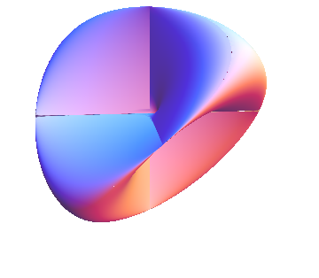
The ${\cal C}_{N}[\mu]$ backgrounds $X$ break $SU(3)_{R}$ to $(U(1)\times U(1))_{K}$ generated by

\displaystyle K_{i}=2\tau_{i}-[H_{\alpha_{i}},\cdot],\quad i=1,2,3\qquad\text{with}\quad K_{1}+K_{2}+K_{3}=0\;.

(2.29)

where $\tau_{i}$ denotes the Cartan generators of $SU(3)_{R}$ . This is a combination of the global $(U(1)\times U(1))_{R}\subset SU(3)_{R}$ symmetry and the $SU(3)_{X}\subset SU(N)$ gauge symmetry. We denote these $U(1)_{K_{i}}$ -charges by

\displaystyle K(\phi)\quad\in\ \mathfrak{s}\mathfrak{u}(3)^{*}

(2.30)

for any⁴⁴ 4 In particular, $K(X_{\alpha})=0$ expresses the invariance of the background. scalar field $\phi$ , and similarly also for fermionic fields. They define a $\mathfrak{s}\mathfrak{u}(3)$ weight lattice. The $\mathfrak{s}\mathfrak{u}(3)_{X}\subset\mathfrak{s}\mathfrak{u}(N)$ gauge charges will be denoted as usual by $\lambda(\phi)\in\mathfrak{s}\mathfrak{u}(3)^{*}$ , so that $K=2\tau-\lambda$ . They all live in the same $\mathfrak{s}\mathfrak{u}(3)$ weight lattice. Furthermore, we will need the $\tau$ -parity generator $\tau$ in $U(3)_{R}$ defined by

\displaystyle\tau\phi_{i}^{\pm}=\pm\phi_{i}^{\pm}\ ,

(2.31)

which is broken by the cubic potential (2.7).

Minimal branes.

The simplest solutions are the minimal branes, which arise for $\mu=(1,0)$ and $\mu=(0,1)$ . To see e.g. ${\cal C}[(1,0)]$ explicitly, denote the 3 extremal weight vectors of $(1,0)$ with $\{|1,\mu\rangle,|2,\mu\rangle,|3,\mu\rangle\}$ . Then the minimal squashed $\mathds{C}P^{2}$ brane is given by

\displaystyle X_{i}^{+}

\displaystyle\coloneqq T_{i}^{+}=|i,\mu\rangle\langle i-1,\mu|

(2.32)

where $T$ is the fundamental representation of $\mathfrak{s}\mathfrak{u}(3)$ , and we dropped $r$ for simplicity. The energy for this minimal brane for $M_{i}=0$ is obtained using (2.22) as

\displaystyle V_{4}+V_{3}=\frac{1}{4}V_{3}=-2\mbox{tr}(T_{1}^{+}[T_{2}^{+},T_{3}^{+}]+\text{h.c.})=-8\ .

(2.33)

2.3 Geometric significance: self-intersecting branes

The qualitative features of the above solutions, and in particular the chirality properties of the fermionic zero modes discussed below, can be understood in terms of the semi-classical geometry of the solutions, interpreted as self-intersecting branes in $\mathds{R}^{6}$ . As for all quantized coadjoint orbits, the semi-classical geometry of ${\cal C}_{N}[\mu]$ can be extracted using coherent states. These are precisely the $SU(3)$ orbits $\{g\cdot|x\rangle\,,\;g\in SU(3)\}$ of the extremal weight states $|x\rangle$ of the irreps ${\cal H}_{\Lambda}\in\mathrm{End}({\cal H}_{\mu})$ , where ${\cal H}_{\mu}$ is the representation space for the $\mathfrak{s}\mathfrak{u}(3)$ representation $\pi_{\mu}$ . The set of coherent states $|gx\rangle\coloneqq g\cdot|x\rangle$ forms a $U(1)$ bundle over the coadjoint orbit ${\cal O}[\mu]$ , and the semi-classical base manifold embedded in $\mathds{R}^{6}$ (the brane) is recovered from the expectation values of these coherent states

\displaystyle{\cal C}

\displaystyle=\left\{\langle gx|X^{\alpha}|gx\rangle,\ g\in SU(3)\right\}\subset\mathds{R}^{6}.

(2.34)

This would be the full coadjoint orbit ${\cal O}[\mu]$ if the $X^{\alpha}$ were supplemented by the Cartan generators $H_{3},H_{8}$ , but here we obtain the projection ${\cal C}[\mu]$ of ${\cal O}[\mu]$ along the Cartan generators, cf. [25, 27, 26].

The extremal weight states ${\cal W}|x\rangle$ , which lie on the discrete orbit of the Weyl group ${\cal W}$ through $|x\rangle$ , are projected to the origin of weight space. To see this, it is sufficient to note that $\langle x|X_{\alpha}|x\rangle=0$ as any $X_{j}^{\pm}$ annihilates either $|x\rangle$ or $\langle x|$ . The tangent space of the sub-variety ${\cal C}_{N}[\mu]$ is obtained by acting with the three $SU(2)_{\alpha}$ subgroups, which correspond to the roots $X_{\alpha}$ of $\mathfrak{s}\mathfrak{u}(3)$ , on the set of extremal weight states ${\cal W}|x\rangle$ . For $\mu=(N,0)$ and $\mu=(0,N)$ , one of these actions vanishes, leading to the 4-dimensional self-intersecting $\mathds{C}P^{2}$ branes depicted in figure 1(b). For generic $\mu=(N_{1},N_{2})$ , the ${\cal C}_{N}[\mu]$ are 6-dimensional sub-varieties in $\mathds{R}^{6}$ , i.e. they are locally space-filling branes. Moreover, the non-degenerate Poisson structure on ${\cal C}_{N}[\mu]$ is recovered from the commutators $[X^{\alpha},X^{\beta}]\sim i\{x^{\alpha},x^{\beta}\}$ , whose Pfaffian is measured by the operator $\chi$ , see (4.1). Therefore the generic 6-dimensional branes, which carry a rank 6 flux due to the symplectic form, consist of 3+3 locally space-filling sheets that cover the origin.

2.4 Fluctuations and zero modes

Consider the fluctuations of the scalar fields on a background brane ${\cal C}[\mu]$ with representation space ${\cal H}$ . To organize the degrees of freedom $\mathrm{End}({\cal H})$ , which denotes the algebra of all possible functions, we note that the solutions (2.23) define an embedding $SU(3)_{X}\subset SU(N)$ , which acts via the adjoint on all the fields. Consequently, we decompose the $\mathfrak{s}\mathfrak{u}(N)$ -valued fields into harmonics, i.e. irreps of this $SU(3)_{X}$

\displaystyle\mathfrak{s}\mathfrak{u}(N)\cong\mathrm{End}({\cal H})\big|_{SU(3)_{X}}=\oplus_{\Lambda}n_{\Lambda}{\cal H}_{\Lambda}

(2.35)

where ${\cal H}_{\Lambda}$ denotes the irreps with highest weight $\Lambda$ appearing with multiplicity $n_{\Lambda}$ . For the case of $\mu=(N,0)$ or $\mu=(0,N)$ , this decomposition is given by

\displaystyle\mathrm{End}({\cal H})\big|_{SU(3)_{X}}=\oplus_{n=0}^{N}{\cal H}_{(n,n)}\ .

(2.36)

While the $SU(3)_{X}$ gauge transformations do not act on the indices $\alpha$ of the scalar fields $\phi_{\alpha}$ , the $(U(1)\times U(1))_{K_{i}}$ symmetry (2.29) does act, and the $\alpha$ realize 3+3 of the 8 states in $(1,1)$ of the $\mathfrak{s}\mathfrak{u}(3)$ weight lattice due to the origin of ${\cal C}[\mu]$ as a $SU(3)$ coadjoint orbit. This allows to organize the various harmonics, which will be very useful.

Assume first $M_{i}=0$ . Then the squashed brane backgrounds $X_{\alpha}$ admit a number of bosonic zero modes $\phi^{(0)}_{\alpha}$ , as shown in [25]. To see this, we note that the bilinear form defined by $\not{D}_{\rm mix}$ on a background (2.23) can be simplified, for example, as follows:

\displaystyle\mbox{tr}\big(\phi_{i}^{-}(\not{D}_{\rm mix}\phi)^{+}_{i}\big)

\displaystyle=\sum_{j\neq i}\mbox{tr}(\phi_{i}^{-}[[X_{i}^{+},X_{j}^{+}],\phi_{j}^{-}])=-\varepsilon_{ikj}\frac{R_{i}R_{j}}{R_{k}}\mbox{tr}(\phi_{i}^{-}[X_{k}^{-},\phi_{j}^{-}])

(2.37)

using (2.26a), where the $\phi_{j}^{\pm}$ are perturbations as in (2.15). For $R_{i}\equiv R$ , this has the form of the quadratic contribution from the cubic potential (2.16), and the quadratic terms in the potential can be combined as follows:

	$\displaystyle V_{2}[\phi]=\frac{1}{2}\mbox{tr}\phi^{\alpha}{\cal O}_{V}^{X}\phi_{\alpha}\ ,\qquad{\cal O}_{V}^{X}$	$\displaystyle\stackrel{{\scriptstyle R_{i}=R}}{{=}}\Box_{X}+2\not{D}_{\rm diag}+2(1-\frac{2}{R})\not{D}_{\rm mix}\$
		$\displaystyle\stackrel{{\scriptstyle R_{i}=1}}{{=}}\Box_{X}+2\not{D}_{\rm diag}-2\not{D}_{\rm mix}\ .$		(2.38)

It has been proven in [25] that, under these conditions, ${\cal O}_{V}^{X}$ is positive semi-definite for all representations $\pi$ . The zero modes of ${\cal O}_{V}^{X}$ fall into two classes, denoted as regular and exceptional zero modes. We will focus on the regular zero modes, and show that their classification is based on a decoupling condition, as discussed in the next section.

2.5 Regular zero modes and decoupling condition

Let $\phi_{\alpha}$ and $\psi_{\alpha},\ \alpha\in{\cal I}$ be two arbitrary matrix configurations, each consisting of three complex matrices or equivalently six hermitian matrices. We will say that $\phi_{\alpha}$ and $\psi_{\alpha}$ satisfy the decoupling condition if

\displaystyle[\psi_{\alpha},\phi_{\beta}]=0\qquad\mbox{whenever}\quad\alpha+\beta\in{\cal I}\quad\mbox{or}\ \ \alpha+\beta=0

(2.39)

This condition is symmetric under $\psi\leftrightarrow\phi$ , and equivalent to

\displaystyle[\psi_{\alpha},\phi_{-\beta}]=0\qquad\mbox{whenever}\quad\alpha-\beta\in{\cal I}\quad\mbox{or}\ \ \alpha-\beta=0\ .

(2.40)

We define regular zero modes $\phi_{\alpha}$ of ${\cal O}_{V}^{X}$ to be modes that satisfy the decoupling condition w.r.t. $X_{\alpha}$ . As we will see momentarily, these modes are in fact zero modes of ${\cal O}_{V}^{X}$ for $R_{i}=R$ and $M_{i}=0$ , and this definition is then equivalent to the one given in [25, 27]. The conditions (2.39) or (2.40) amount to the requirement that $\phi_{\alpha}$ is annihilated by three ladder operators out of the six $X_{j}^{\pm}$ . For example, the condition for $\phi_{i}^{+}$ is

\displaystyle[X_{j}^{+},\phi_{i}^{+}]

\displaystyle=0\quad\text{for}\ \ j\neq i,\quad\text{and}\quad[X_{i}^{-},\phi_{i}^{+}]=0\quad\text{(no sum)}.

(2.41)

Before classifying them more explicitly, we state some important consequences. For $M_{i}=0$ , the regular zero modes $\phi_{\alpha}$ satisfy

	$\displaystyle(\not{D}_{\rm mix}^{X}\phi)_{i}^{+}$	$\displaystyle=0$		(2.42)
	$\displaystyle{\cal O}_{V,M_{i}\equiv 0}^{X}\phi_{i}^{+}$	$\displaystyle=[H_{R},\phi_{i}^{+}]\ \stackrel{{\scriptstyle R_{i}=R}}{{=}}\ 0$		(2.42)

where

\displaystyle H_{R}

\displaystyle\coloneqq R_{1}^{2}H_{1}+R_{2}^{2}H_{2}+R_{3}^{2}H_{3}\ \stackrel{{\scriptstyle R_{i}=R}}{{=}}\ 0\ .

(2.43)

To prove the first statement of (2.42), consider

	$\displaystyle(\not{D}_{\rm mix}^{X}\phi)_{i}^{+}$	$\displaystyle=\sum_{j}[[X_{i}^{+},X_{j}^{+}],\phi_{j}^{-}]+\sum_{j\neq i}[[X_{i}^{+},X_{j}^{+}],\phi_{j}^{+}]$
		$\displaystyle=\sum_{j,k}\frac{R_{i}R_{j}}{R_{k}}\varepsilon_{ijk}\underbrace{[X_{k}^{-},\phi_{j}^{-}]}_{=0}-\sum_{j\neq i}[\underbrace{[X_{j}^{-},\phi_{j}^{+}]}_{=0},X_{i}^{+}]-\sum_{j\neq i}[\underbrace{[\phi_{j}^{+},X_{i}^{+}]}_{=0},X_{j}^{-}]=0$		(2.44)

where we have used the algebra relation (2.26a) and the Jacobi identity. All indicated commutators vanish due to decoupling condition (2.41). For the second statement of (2.42), consider

$\displaystyle\Box_{X}\phi_{i}^{+}$	$\displaystyle=\sum_{j}[X_{j}^{+},[X_{j}^{-},\phi_{i}^{+}]]+\sum_{j}[X_{j}^{-},[X_{j}^{+},\phi_{i}^{+}]]=\sum_{j\neq i}[X_{j}^{+},[X_{j}^{-},\phi_{i}^{+}]]+[X_{i}^{-},[X_{i}^{+},\phi_{i}^{+}]]$
	$\displaystyle=\sum_{j\neq i}[[X_{j}^{+},X_{j}^{-}],\phi_{i}^{+}]-[[X_{i}^{+},X_{i}^{-}],\phi_{i}^{+}]=\sum_{j\neq i}R_{j}^{2}[H_{j},\phi_{i}^{+}]-R_{i}^{2}[H_{i},\phi_{i}^{+}]$	(2.45)
$\displaystyle\not{D}_{\rm diag}\phi_{i}^{+}$	$\displaystyle=R_{i}^{2}[[T_{i},T_{-i}],\phi_{i}^{+}]=R_{i}^{2}[H_{i},\phi_{i}^{+}]\$	(2.46)

using (2.41). Therefore

\displaystyle{\cal O}_{V,M_{i}\equiv 0}^{X}\phi_{i}^{+}=(\Box_{X}+2\not{D}_{\rm diag})\phi_{i}^{+}=[H_{R},\phi_{i}^{+}]\stackrel{{\scriptstyle R_{i}=R}}{{=}}0

(2.47)

Consequently, the regular zero modes, as defined by the decoupling condition, are indeed zero modes of the $SU(3)$ branes if all $R_{i}$ are equal and all mass parameters $M_{i}$ vanish. We shall keep this name also in the general case of non-vanishing masses and distinct $R_{i}$ , which is discussed in section 3.1.3.

Now we relate this to the group-theoretical classification of the regular zero modes on a squashed $SU(3)$ brane ${\cal C}[\mu]$ given in [25, 26]. The decoupling conditions imply that any regular zero mode $\phi_{\alpha}$ for any fixed $\alpha\in{\cal I}$ is an extremal weight vector with $\mathfrak{s}\mathfrak{u}(3)_{X}$ weight $\lambda$ in some irrep ${\cal H}_{\Lambda}\subset\mathrm{End}({\cal H})$ of the decomposition (2.35). In view of (2.41), the arrow $\lambda$ must be the extremal weight vector in the Weyl chamber opposite to the polarization $\alpha$ (or possibly on its wall). Recalling the unbroken $U(1)_{K_{i}}$ of the background, this means that it is one of the six extremal $U(1)_{K_{i}}$ weights⁵⁵ 5 These are the corners of the convex set of weights, or equivalently of the maximal $\mathfrak{s}\mathfrak{u}(3)$ irrep in $(1,1)\otimes{\cal H}_{\Lambda^{+}}$ . $\Lambda^{\prime}=\alpha-\lambda$ of any $\phi_{\alpha}\in{\cal H}_{\Lambda}$ , and we denote it by

\displaystyle\phi_{\alpha,\Lambda^{\prime}}\ \in{\cal H}_{\Lambda},\qquad\Lambda^{\prime}=\alpha-\lambda\equiv K(\phi_{\alpha,\Lambda^{\prime}})\ .

(2.48)

Hence the regular zero modes $\phi_{\alpha,\Lambda^{\prime}}$ have charge $\Lambda^{\prime}=\alpha-\lambda$ under the $K_{i}$ , corresponding to a point of the $\mathfrak{s}\mathfrak{u}(3)$ weight lattice in (the interior of) the Weyl chamber of $\alpha$ . The eigenvalue $\tau=\pm 1$ determined by the parity of the Weyl chamber of $\alpha=\pm\alpha_{i}$ . Clearly there is only one (extremal) state in ${\cal H}_{\Lambda}$ for any such $\Lambda^{\prime}$ . Since ${\not{D}}_{\rm mix}$ preserves $\Lambda^{\prime}$ but flips the $\tau$ -parity (recalling $\tau{\not{D}}_{\rm mix}=-{\not{D}}_{\rm mix}\tau$ from [26]), it follows again that $\not{D}_{\rm mix}^{X}\phi=0$ , i.e. (2.42) holds. This provides another way to characterize the regular zero modes.

We now observe that the regular zero modes form a ring, in the following sense: For each $\alpha$ , let $V_{\alpha}=\{\phi_{\alpha,\Lambda^{\prime}}\}$ be the vector space of regular zero modes with polarization $\alpha$ . According to (2.48), this vector space is graded by the integral weights in the Weyl chamber corresponding to $\alpha$ . Moreover, the decoupling condition (2.39) – or equivalently the extremal weight property – implies that if $\phi_{\alpha}$ , $\phi^{\prime}_{\alpha}$ are regular zero modes with the same polarization $\alpha$ , then so is their (matrix) product $\phi_{\alpha}\phi^{\prime}_{\alpha}$ . Hence, each $V_{\alpha}$ is a graded ring. Moreover, the vector space $V=\oplus_{\alpha}V_{\alpha}$ forms a ring graded by the (integral) weights of $\mathfrak{s}\mathfrak{u}(3)$ (or rather of $U(1)_{K_{i}}$ ), where we define the product of zero modes in different Weyl chambers to vanish⁶⁶ 6 This does not mean that their matrix product vanishes. However, this concept helps to organize the regular zero modes. This structure is respected by the Weyl group ${\cal W}$ , which relates the different $V_{\alpha}$ . In particular, all ring elements are nilpotent, due to the cutoff in $\Lambda$ .

The same analysis goes through for stacks of branes, where analogous zero modes arise as strings connecting different branes. As aforementioned, we will denote the space of zero modes as Higgs sector. Labeling the six-component vector $\phi=(\phi_{\alpha})$ of zero modes by the dominant $U(1)_{K_{i}}$ weight, we learn that the Higgs sector forms a nilpotent ring graded by integral weights of $\mathfrak{s}\mathfrak{u}(3)$ .

Examples.

Starting from the simplest solution to the decoupling condition

\displaystyle\phi_{\alpha,\alpha}=T_{-\alpha}

(2.49)

one can use the ring multiplication of the regular zero modes to construct modes of the form

\displaystyle\phi_{\alpha,(n+1)\alpha}=(T_{-\alpha})^{n},

(2.50)

and any linear combinations of these. A possible background with such a zero mode would then be

\displaystyle Y_{\alpha}=X_{\alpha}+\varepsilon_{\alpha}(T_{-\alpha})^{n}.

(2.51)

On a single squashed $\mathds{C}P^{2}_{N}$ brane ${\cal C}[(N,0)]$ , these exhausts all regular zero modes. The ring structure is given by $V_{\alpha}=\mathds{C}[\phi_{\alpha,\alpha}]/\langle\phi_{\alpha,\alpha}^{N+1}\rangle$ . In particular, the regular zero modes with maximal $n=N$ on squashed $\mathds{C}P^{2}_{N}$ link the 3 intersecting $\mathds{R}^{4}$ sheets at the origin, with polarization along the common $\mathds{R}^{2}$ [25]. These string-modes are given by $|i-1,\mu\rangle\langle i,\mu|$ , where $\{|1,\mu\rangle,|2,\mu\rangle,|3,\mu\rangle\}$ denote the 3 extremal weight vectors of $\mu=(N,0)$ . These are coherent states located at the origin on each of the three sheets. An artist’s rendering of such a string mode underlying this solution is given in figure 1(b). More generally, the regular zero modes can be interpreted as strings linking these sheets, shifted along their intersection.

Exceptional zero modes.

In addition to the regular zero modes, there are certain exceptional zero modes which are described in [25, 26]. For the squashed $\mathds{C}P^{2}_{N}$ solutions, the only exceptional modes are the six Goldstone bosons corresponding to the spontaneously broken $SU(3)/\penalty(U(1)\times U(1))$ . These are easily understood also in the deformed settings considered below. For the more general branes, the explicit description of the exceptional zero modes is not known. This is one reason why we focus mostly on the $\mathds{C}P^{2}$ branes in this paper.

$\mathds{Z}_{3}$ and generations.

Note that the $U(3)_{R}$ label $\alpha$ for the scalar fields determines a 3-family structure, which reflects the Weyl group $\mathds{Z}_{3}\times\mathds{Z}_{2}={\cal W}$ . This coincides with the family and the $\tau$ -parity as determined by the $U(1)_{i}$ charges of the zero modes. The $\mathds{Z}_{3}\times\mathds{Z}_{2}$ structure is indicated by the field labels as in $\phi_{i\pm}$ . This will be useful for selection rules etc.

Stringy versus semi-classical modes.

The above characterization of regular zero modes hides the fact that they come with very different characteristics. We single out two extreme types: (i) the maximal or stringy zero modes, and (ii) the semi-classical or almost-commutative zero modes. The distinction corresponds to the separation of functions on non-squashed $SU(3)$ coadjoint orbits ${\cal C}[\mu]$ into UV and IR sector, as discussed in [32], but they are also distinguished by their coupling strength:

All Higgs modes couple to all other (scalar, gauge and fermionic) fields through commutators $[\phi_{\alpha},\cdot]$ . To quantify this strength, we first need to proper normalize the Higgs modes. This is dictated by the kinetic term⁷⁷ 7 the canonical form is obtained by absorbing $g$ in the scalar field $\phi_{a}$ .

\displaystyle-\int d^{4}x\ \frac{1}{2g^{2}}\mbox{tr}(D^{\mu}\phi^{a}D_{\mu}\phi_{a})

(2.52)

i.e. all modes should be normalized w.r.t. the trace $\mbox{tr}()$ . Now the maximal Higgs modes $\phi^{\mathrm{string}}_{\alpha,\Lambda^{\prime}}$ are the ones with extremal $\mathfrak{s}\mathfrak{u}(3)_{K}$ weight $\Lambda^{\prime}$ ; these modes are given by rank one operators

\displaystyle\phi^{\mathrm{string}}_{\alpha,\Lambda^{\prime}}=|x\rangle\langle x^{\prime}|

(2.53)

linking the extremal (i.e. coherent) weight states $|x\rangle$ , $|x^{\prime}\rangle$ of ${\cal H}_{\Lambda}\subset\mathrm{End}({\cal H})$ whose weight difference is maximal. From the brane point of view, these are the extreme UV modes with the maximal momentum [32]. Since the expectation values vanish, $\langle x|X_{\alpha}|x\rangle=0$ , these states are localized at the origin, and $\phi^{\rm string}$ should be interpreted as strings linking the sheets of squashed ${\cal C}[\mu]$ at the origin. For large $N$ , there are other almost-maximal zero modes, for example with rank 2 such as the modes considered in section 4. These almost-maximal modes have a similar properties as the maximal modes; hence, this broader class will be called stringy modes. The commutator of these zero modes is of order one,

\displaystyle[\phi_{\alpha}^{\mathrm{string}},\phi_{\beta}^{\mathrm{string}}]=O(1)

(2.54)

i.e. they are completely non–commutative functions on the branes. Putting back $g$ (2.52), we see that their interaction strength is characterized by $g$ .

In contrast, the zero modes $\phi^{\rm low}_{\alpha,\Lambda^{\prime}}$ with small weight $\Lambda^{\prime}$ are matrices with high, typically maximal rank. These modes correspond to slowly-varying, semi-classical functions $\phi^{\rm low}_{\alpha,\Lambda^{\prime}}(x)$ on the ${\cal C}[\mu]$ brane, given by polynomials of small degree in the $X_{\alpha}$ , the lowest mode being

\displaystyle\phi_{\alpha}=\frac{1}{c_{N}}X_{-\alpha}\ \sim\frac{1}{c_{N}}x_{-\alpha}\ .

(2.55)

The normalization $c_{N}$ for the minimal zero mode on an irreducible ${\cal C}[\mu]$ can be obtained from the quadratic Casimir on ${\cal H}_{\mu}$ ,

\displaystyle 1=\mbox{tr}(\phi_{a}\phi_{a})=\frac{r^{2}}{c_{N}^{2}}\,\mbox{tr}(T_{a}T_{a})=\frac{r^{2}}{c_{N}^{2}}\,\frac{\dim({\cal H}_{\mu})}{4}(\mu,\mu+2\rho)\quad\text{(no sum)}\,.

(2.56)

Thus

\displaystyle c_{N}^{2}=\frac{r^{2}\dim({\cal H}_{\mu})}{4}(\mu,\mu+2\rho)=O(N^{2})\,,

(2.57)

which means that the $\phi_{a}$ are almost-commutative functions on ${\cal C}[\mu]$ ,

\displaystyle[\phi_{\alpha}^{\mathrm{low}},\phi_{\beta}^{\mathrm{low}}]=\frac{1}{c_{N}^{2}}c_{\alpha\beta}^{a}T_{a}\

\displaystyle\sim i\{\phi_{\alpha}^{\mathrm{low}},\phi_{\beta}^{\mathrm{low}}\}\ \ll 1

(2.58)

where $\{\cdot,\cdot\}$ denotes the Poisson bracket, as usual for low-energy functions on fuzzy spaces. Hence their interaction strength is small, and they are become free fields as $N\to\infty$ .

To summarize, the vast number of scalar modes for large $N$ becomes gapped on an irreducible ${\cal C}[\mu]$ vacuum, and the zero modes consist of stringy modes with interaction strength $g$ , as well as weakly interacting semi-classical modes. We will see below that the stringy modes form bound states which are stable at least for a special value of the mass parameter, in which case the zero modes are further reduced to a small number independent of $N$ .

2.6 Aspects of the Higgs potential

Now consider the interacting potential for the Higgs sector, i.e. the zero modes $\phi_{\alpha}$ on a background solution $X$ . The linear term in $\phi$ vanishes due to the eom for $X$ , so that the effective potential for $\phi$ obtained from (2.16) is

	$\displaystyle V_{\mathrm{eff}}[\phi]$	$\displaystyle\coloneqq V[X+\phi]-V[X]$		(2.59)
		$\displaystyle=V[\phi]+\mbox{tr}\left(\frac{1}{2}\phi^{\alpha}\big(\Box_{X}+2{\not{D}}_{\rm diag}\big)\phi_{\alpha}+(X^{\alpha}+\frac{1}{4}\phi^{\alpha})\Box_{\phi}\phi_{\alpha}-\frac{1}{2}f^{2}\right)\;.$		(2.59)

For the regular zero modes, the cubic interaction $V_{31}$ arising from the quartic term drops out. To see this, consider

$\displaystyle V_{31}\ \ni\ \mbox{tr}X^{\alpha}\Box_{\phi}\phi_{\alpha}$	$\displaystyle=\mbox{tr}[X_{\alpha},\phi_{\beta}][\phi^{\alpha},\phi^{\beta}]\qquad\qquad\mbox{(no sum)}$
	$\displaystyle=-\mbox{tr}\phi_{\beta}[[\phi^{\alpha},\phi^{\beta}],X_{\alpha}]=\mbox{tr}\phi_{\beta}\Big([[\phi^{\beta},X_{\alpha}],\phi^{\alpha}]+[[X_{\alpha},\phi^{\alpha}],\phi^{\beta}]\Big)$
	$\displaystyle=-\mbox{tr}\phi_{\beta}[[\phi_{-\beta},X_{\alpha}],\phi^{\alpha}]$	(2.60)

using the Jacobi identity, $\phi^{\beta}=\phi_{-\beta}$ , and the gauge-fixing condition $f=[X_{\alpha},\phi^{\alpha}]=0$ , which follows from the decoupling condition (2.39). Since either $\alpha\pm\beta\in{\cal I}$ or $\alpha\pm\beta=0$ for any pair of roots $\alpha,\beta$ of $\mathfrak{s}\mathfrak{u}(3)$ , the $V_{31}$ term (2.60) vanishes for the regular zero-modes, again due to the decoupling condition. Therefore $V_{\mathrm{eff}}[\phi]$ reduces for the regular zero mode sector to

\displaystyle V_{\mathrm{eff}}[\phi]

\displaystyle=V[\phi]+\mbox{tr}\left(\frac{1}{2}\phi^{\alpha}\big(\Box_{X}+2{\not{D}}_{\rm diag}^{X}\big)\phi_{\alpha}\right)\,.

(2.61)

The second term is nothing else than $\frac{1}{2}\mbox{tr}(\phi^{\alpha}{\cal O}_{V,M_{i}\equiv 0}^{X}\phi_{\alpha})$ and vanishes since $\phi_{\alpha}$ are regular zero modes, see (2.42). Hence, the effective potential for the regular zero modes is given by

\displaystyle{\cal V}[\phi]

\displaystyle=\frac{m^{4}}{g^{2}}V[\phi]=\frac{m^{4}}{g^{2}}\mbox{tr}\left(V_{4}[\phi]+V_{\rm soft}[\phi]\right)

(2.62)

and we arrive at

\displaystyle{\cal V}[X+\phi]={\cal V}[X]+{\cal V}[\phi]\ .

(2.63)

We emphasize that the argument remains valid for any element of the ring of regular zero modes: suppose $\phi$ and $\phi^{\prime}$ are two six-component vectors of regular zero modes, then

\displaystyle{\cal V}[X+(\phi+\phi^{\prime})]={\cal V}[X]+{\cal V}[\phi+\phi^{\prime}]\quad\text{and}\quad{\cal V}[X+(\phi\cdot\phi^{\prime})]={\cal V}[X]+{\cal V}[\phi\cdot\phi^{\prime}]

(2.64)

holds, with the component-wise multiplication defined in section 2.5. However, ${\cal V}[\phi+\phi^{\prime}]$ or ${\cal V}[\phi\cdot\phi^{\prime}]$ do not necessarily decompose in any linear fashion. Similarly, one can extend to discussion to Higgs modes connecting stacks of branes and the argument remains the same.

In particular, the potential for $\phi$ has the same structure as the original potential (2.6) for the model. Thus the quadratic potential $V_{2}[\phi]$ vanishes again in the absence of mass terms, but the cubic term $V_{3}[\phi]$ may entail some unstable directions. Some of the $\phi_{\alpha}$ are then expected to take a non-trivial VEV, which is then stabilized by the quartic term. We will indeed find such non-trivial minima for $\phi_{\alpha}$ , which will be denoted as Higgs vacua. Such a non-trivial Higgs linking different branes leads to a bound state of the branes.

As a further remark, we note that the mixed term quadratic in both $X$ and $\phi$ can be written equivalently as

\displaystyle\mbox{tr}\Big(\phi^{\alpha}\big(\Box_{X}+2{\not{D}}_{\rm diag}^{X}\big)\phi_{\alpha}\Big)=\mbox{tr}\Big(X^{\alpha}\big(\Box_{\phi}+2{\not{D}}_{\rm diag}^{\phi}\big)X_{\alpha}\Big)

(2.65)

assuming the decoupling condition between $\phi$ and $X$ .

The above argument for (2.60) to vanish does not apply to the exceptional zero modes. For single branes of $\mathds{C}P^{2}$ type, these are precisely the $SU(3)_{R}$ Goldstone bosons, which can be studied separately. However there exist other exceptional zero modes, e.g. $\Lambda\in{\cal W}(1,0),\ \Lambda^{\prime}\in{\cal W}(2,0)$ (or conjugate) connecting ${\cal C}[(0,1)]$ with ${\cal C}[(1,0)]$ which need to be studied separately.

We will see that in the presence of positive mass terms $M_{i}^{2}>0$ , the above instability can be stabilized. However if the $M^{2}_{i}$ are not all equal, some of the $\phi^{\alpha}$ turn out to acquire a negative mass. This will also lead to a non-trivial Higgs vacuum. Quantum corrections⁸⁸ 8 Another conceivable mechanism is a rotation of the branes, see [27]. might also play an important role, however we will assume that these are subleading if the branes are sufficiently large, so that the semi-classical description is valid.

Full equations of motion and decoupling.

We have just seen that ${\cal V}(X+\phi)={\cal V}(X)+{\cal V}(\phi)$ for a sum of backgrounds $X$ , $\phi$ satisfying the decoupling condition (2.39). Now, we would like to know if such a composed background $Y^{\alpha}=X^{\alpha}+\phi^{\alpha}$ can be an exact solution of the full action. To address this, we cannot rely on the above reduced action for the Higgs sector, because we need $\delta S=0$ for arbitrary fluctuations of $Y^{\alpha}$ .

Consider combined (static) configurations of the form $X^{a}+\phi^{a}$ which satisfies the equation of motion

\displaystyle 0=(\Box_{X+\phi}+4M_{i}^{2})\big)(X+\phi)_{i}^{+}+4\varepsilon_{ijk}(X+\phi)_{j}^{-}(X+\phi)_{k}^{-}.

(2.66)

To simplify this, consider the matrix Laplacian $\Box_{X+\phi}$ acting on an arbitrary $\psi\in\mathrm{End}({\cal H})$ . We obtain

	$\displaystyle\Box_{X+\phi}\psi$	$\displaystyle=(\Box_{\phi}+\Box_{X})\psi+[X_{\beta},[\phi^{\beta},\psi]]+[\phi_{\beta},[X^{\beta},\psi]]$
		$\displaystyle=(\Box_{\phi}+\Box_{X})\psi+2[\phi_{\beta},[X^{\beta},\psi]]-[\psi,[X_{\beta},\phi^{\beta}]]\;.$		(2.67)

Applying this on $X+\phi$ leads to

$\displaystyle\Box_{X+\phi}(X_{\alpha}+\phi_{\alpha})$	$\displaystyle=(\Box_{\phi}+\Box_{X})(X_{\alpha}+\phi_{\alpha})+2[\phi_{\beta},[X^{\beta},X_{\alpha}]]+2[X_{\beta},[\phi^{\beta},\phi_{\alpha}]]$
	$\displaystyle\quad-[\phi_{\alpha},[\phi_{\beta},X^{\beta}]]-[X_{\alpha},[X_{\beta},\phi^{\beta}]]$
	$\displaystyle=(\Box_{\phi}+\Box_{X})(X_{\alpha}+\phi_{\alpha})+2({\not{D}}_{ad}^{X}\phi)_{\alpha}+2({\not{D}}_{ad}^{\phi}X)_{\alpha}$
	$\displaystyle\quad-[\phi_{\alpha},[\phi_{\beta},X^{\beta}]]-[X_{\alpha},[X_{\beta},\phi^{\beta}]]\ .$	(2.68)

If $X_{\alpha}$ and $\phi_{\alpha}$ satisfy the decoupling condition (2.39), we can replace ${\not{D}}_{\mathrm{ad}}^{X}\phi={\not{D}}_{\mathrm{diag}}^{X}\phi$ etc., and also $[X_{\beta},Y^{\beta}]=0$ holds. This further simplifies the Laplacian to

\displaystyle\Box_{X+\phi}(X_{\alpha}+\phi_{\alpha})

\displaystyle=(\Box_{\phi}+\Box_{X})(X_{\alpha}+\phi_{\alpha})+2({\not{D}}_{\mathrm{diag}}^{X}\phi)_{\alpha}+2({\not{D}}_{\mathrm{diag}}^{\phi}X)_{\alpha}\ .

(2.69)

Furthermore, we note that the cubic term simplifies via (2.41) to

	$\displaystyle\varepsilon_{ijk}(X+\phi)_{j}^{-}(X+\phi)_{k}^{-}$	$\displaystyle=\varepsilon_{ijk}X_{j}^{-}X_{k}^{-}+\varepsilon_{ijk}\phi_{j}^{-}\phi_{k}^{-}+\varepsilon_{ijk}[X_{j}^{-},\phi_{k}^{-}]$
		$\displaystyle=\varepsilon_{ijk}X_{j}^{-}X_{k}^{-}+\varepsilon_{ijk}\phi_{j}^{-}\phi_{k}^{-}\;.$		(2.70)

Collecting all the intermediate steps, the full eom reduces to

	$\displaystyle 0$	$\displaystyle=\big(\Box_{\phi}+2{\not{D}}_{\rm diag}^{\phi}\big)X_{i}^{+}+\big(\Box_{X}+4M_{i}^{2}\big)X_{i}^{+}+2\varepsilon_{ijk}[X_{j}^{-},X_{k}^{-}]$
		$\displaystyle+\big(\Box_{X}+2{\not{D}}_{\rm diag}^{X}\big)\phi_{\alpha}+\big(\Box_{\phi}+4M_{i}^{2}\big)\phi_{i}^{+}+2\varepsilon_{ijk}[\phi_{j}^{-},\phi_{k}^{-}]$		(2.71)

provided $X$ and $\phi$ satisfy the decoupling conditions (2.39). Now recall that


	$\displaystyle(\Box_{X}+2{\not{D}}_{ad}^{X})\phi_{i}^{+}={\cal O}_{V,M_{i}\equiv 0}^{X}\phi_{i}^{+}=0\quad\text{and}\quad(\Box_{\phi}+2{\not{D}}_{ad}^{\phi})X_{i}^{+}={\cal O}_{V,M_{i}\equiv 0}^{\phi}X_{i}^{+}=0$		(2.72a)

because the symmetry of the decoupling conditions implies that $X$ and $\phi$ are regular zero modes of ${\cal O}_{V,M_{i}\equiv 0}^{\phi}$ and ${\cal O}_{V,M_{i}\equiv 0}^{X}$ , respectively. As a consequence, the full eom for $X+\phi$ reduce to the sum of the individual eom for $X$ and $\phi$ separately. Thus, $X+\phi$ is an exact solution if both $X$ and $\phi$ satisfy their individual equations of motion

\displaystyle\big(\Box_{\phi}+4M_{i}^{2}\big)\phi_{i}^{+}+2\varepsilon_{ijk}[\phi_{j}^{-},\phi_{k}^{-}]=0

(2.73)

and similar for $X$ , as well as the decoupling condition (2.41).

In fact, (2.71) are precisely the eom obtain using the above reduced potential, i.e. dropping the mixed $V_{31}$ terms such as $\phi\Box_{X}X$ and the mixed terms in $V_{3}$ . We can therefore use the reduced potential for backgrounds composed of decoupled solutions. However, note that finding a minimum within the Higgs sector $V(\phi)$ in general implies (2.73) only up to massive modes. This is the reason why we will find exact solutions only in special cases within the maximal Higgs sector.

Furthermore, from the homogeneity of the full potential in either $X$ or $\phi$ , we can infer that $4V_{4}+3V_{3}+2V_{2}=0$ holds at a minimum within the Higgs sector, which implies as in (2.22)

\displaystyle V[\phi]\big|_{\text{sol. eom}}=\frac{1}{4}V_{3}[\phi]+\frac{1}{2}V_{2}[\phi]\ .

(2.74)

This is useful to compare the energy of different solutions.

2.7 Massless versus massive solutions, Higgs condensate, and stability at $M^{*}$

So far, we have restricted the attention mostly to the massless case, i.e. $M_{i}=0$ . This has some immediate implications:

(i)

The eom (2.21) can be solved immediately by the first integral relations $\widetilde{B}_{ij}=0=D$ , which are automatically satisfied on any $SU(3)$ representation $X_{j}^{\pm}=\pi(T_{j}^{\pm})$ .
(ii)

The operator ${\cal O}_{V}^{X}$ governing the dynamics of the bosonic fluctuations is positive semi-definite by virtue of representation theory [25]. This means that there are no instabilities, and moreover there exists a classification of all regular zero modes.
(iii)

The potential energy of the background can be computed by noting that $\widetilde{B_{ij}}=0$ implies $B_{ij}=\frac{1}{3}\varepsilon_{ijk}X_{k}^{-}$ , so that

$\displaystyle V[X]=-\frac{2}{3}\sum_{i}\mbox{tr}(X_{i}^{-}X_{i}^{+})<0\;.$ (2.75)

Now we would like to perturb the background $X$ with regular zero modes $\phi$ to obtain a solution to the full eom for $X+\phi$ , keeping $M_{i}=0$ for the moment. Unfortunately, this is less accessible in general, because

(i)

Since zero modes $\phi$ do not satisfy the $\mathfrak{s}\mathfrak{u}(3)$ Lie algebra, it is not easy to find exact solutions. A notable exception are the maximal regular zero modes on ${\cal C}[(n,0)]$ .
(ii)

The spectrum of the operator ${\cal O}_{V}^{X+\phi}$ is not analytically understood, but numerical studies presented in sections 3–4, and appendix B show the existence of instabilities. Moreover, we do not have a classification of appearing zero modes.

(iii)

Assuming that both $X$ and $\phi$ satisfy the first integral relations $\widetilde{B}_{ij}=0=D$ , the combined potential energy can be evaluate to read

\displaystyle V[X+\phi]=-\frac{2}{3}\sum_{i}\mbox{tr}(X_{i}^{-}X_{i}^{+})-\frac{2}{3}\sum_{i}\mbox{tr}(\phi_{i}^{-}\phi_{i}^{+})<V[X]\;.

(2.76)

Hence starting from a ${\cal C}_{N}[\mu]$ background, the extension to a combined background definitely reduces the potential energy. This strongly suggests the existence of a Higgs condensate.

Let us try to circumvent the appearance of instabilities by including uniform mass parameters $M_{i}\equiv M>0$ and adjusting the radii $R_{i}\equiv R$ in (2.23) accordingly. Starting with $X_{i}^{\pm}$ satisfying $\widetilde{B}_{ij}=0=D$ , the eom (2.21) for the ansatz $Y_{i}^{\pm}=RX_{i}^{\pm}$ reduce to

\displaystyle 0=R\big(R(R-1)+M^{2}\big)X_{i}^{+}\quad\forall i

(2.77)

Thus there are three solutions

\displaystyle R=0\,,\qquad R=\frac{1}{2}(1\pm\sqrt{1-4M^{2}})

(2.78)

for $|M|\leq\frac{1}{2}$ . For these choices of $R$ , the eom are satisfied and we can compute the potential from (2.11), which is

\displaystyle V[Y]=2R^{2}\left(\left(R-\frac{2}{3}\right)^{2}+2\left(M^{2}-\frac{2}{9}\right)\right)\sum_{i}\mbox{tr}(X_{i}^{-}X_{i}^{+})\;.

(2.79)

As discussed in appendix A, for $0<M\leq\frac{\sqrt{2}}{3}$ the solution $R(M)=\frac{1}{2}(1+\sqrt{1-4M^{2}})$ describes the minimal energy configuration. This establishes the following statement (as stated in the introduction): any solution to $\widetilde{B}_{ij}=0=D$ gives rise to a solution to the eom with uniform mass parameter $M$ , provided one rescales with $R(M)$ .

Now we make the following very important observation: for the special mass value

\displaystyle M^{*}\coloneqq\frac{\sqrt{2}}{3}

(2.80)

the full potential (2.11) is positive semi-definite, and the potential vanishes if and only if

\displaystyle B_{ij}=0=D\ .

(2.81)

Upon rescaling, this is equivalent to $\widetilde{B}_{ij}=0=D$ with a radius $R=\frac{2}{3}$ . In particular, the spectrum of ${\cal O}_{V}^{Y}$ is guaranteed to be free of instabilities for any such solution. We will indeed find a number of nontrivial brane plus Higgs solution of this type, which are thereby local minima up to a compact moduli space. This statement is clearly reminiscent of the situation in supersymmetry, even though SUSY is explicitly broken by the potential.

2.8 Gauge fields and mode decomposition

Now consider the gauge fields $A_{\mu}(y)\in\mathrm{End}({\cal H})$ on $\mathds{R}^{4}$ , which together with the gauginos constitute the ${\cal N}=1$ vector superfield in ${\cal N}=4$ SYM. The gauge fields take values in $\mathfrak{s}\mathfrak{u}(N)$ , and accordingly decompose

\displaystyle A_{\mu}=A_{\mu;\Lambda m}(y)Y_{\Lambda m}

(2.82)

into eigenmodes $Y_{\Lambda m}$ of the matrix Laplacian $\Box_{X}$ on squashed ${\cal C}_{N}[\mu]$ background. These modes acquire a mass due to the Higgs effect, given by [25]

	$\displaystyle-\mbox{tr}[X^{a},Y_{\Lambda m}][X_{a},Y_{\Lambda m}]$	$\displaystyle=\mbox{tr}(Y_{\Lambda m}^{\dagger}\Box_{X}Y_{\Lambda m})=m^{2}_{\Lambda,m}$
	$\displaystyle m^{2}_{\Lambda,m}$	$\displaystyle=2r^{2}\big((\Lambda,\Lambda+2\rho)-(m,m)\big)$		(2.83)

assuming the normalization

\displaystyle\mbox{tr}(Y_{\Lambda^{\prime}m^{\prime}}^{\dagger}Y_{\Lambda m})=\delta_{\Lambda m}^{\Lambda^{\prime}m^{\prime}}.

(2.84)

In contrast to the scalar fields, there are no zero modes, and the gauge symmetry is broken completely on an irreducible brane. The lowest of these modes are given by $Y_{\Lambda m}=\frac{1}{c_{N}}X_{\alpha}$ , and the corresponding KK mass scale is of order

\displaystyle m^{2}_{KK}\ \sim\ \frac{r^{2}}{g^{2}}m^{2}

(2.85)

re-inserting the YM coupling constant $g^{2}$ and the cubic coupling $m^{2}$ in the potential (2.6).

Now consider the coupling of the above gauge modes to the Higgs modes or to the fermions. We recall from section 2.5 that the Higgs modes arise in different types, in particular (i) maximal (stringy) modes $\phi_{\alpha}^{\rm string}$ , and (ii) semi-classical modes $\phi_{\alpha}^{\rm low}$ . A similar classification applies to the gauge modes and fermions. The effective coupling strength depends strongly on the type of modes. For the semi-classical gauge modes (these will include $W$ -like bosons discussed in section 6), the coupling to a stringy Higgs mode $\phi^{\rm string}=r_{s}|x\rangle\langle x^{\prime}|$ (2.53) has the structure

\displaystyle[Y_{\Lambda m},\phi^{\rm string}]\approx(Y_{\Lambda m}(x)-Y_{\Lambda m}(x^{\prime}))\phi^{\rm string}

(2.86)

leading to the mass term

\displaystyle-\mbox{tr}[\phi^{\rm string},Y_{\Lambda m}][\phi^{\rm string},Y_{\Lambda m}]

\displaystyle\approx|Y_{\Lambda m}(x)-Y_{\Lambda m}(x^{\prime})|^{2}\mbox{tr}(\phi^{\rm string}\phi^{\rm string})=|Y_{\Lambda m}(x)-Y_{\Lambda m}(x^{\prime})|^{2}

(2.87)

Hence such stringy Higgs give a contribution to the mass of nontrivial gauge boson modes, which is proportional to the difference of the wave function $Y_{\Lambda m}(x)$ at the two ends of the string. However this contribution is suppressed⁹⁹ 9 In contrast, the coupling of the $\phi^{\rm string}$ to the stringy fermions is not suppressed. by the localization (due to (2.84)), and the main contribution to the mass of the gauge bosons arises from the background (2.83).

These observations will apply in particular for the chiral $A_{\mu}\sim\chi$ gauge mode (4.8) on 6-dimensional branes.

Nonabelian case.

As usual, unbroken nonabelian gauge fields arise on stacks of coincident branes. E.g. on a stack of two coinciding branes, the gauge modes have the structure

\displaystyle A_{\mu}=A_{\mu;\Lambda m}(x)Y_{\Lambda m}\otimes\sigma_{i}

(2.88)

where $\sigma_{i}\in\mathfrak{s}\mathfrak{u}(2)$ act on the two branes. Using $Y_{\Lambda m}=\frac{1}{\sqrt{\dim{\cal H}}}\mathds{1}$ for the massless modes, the corresponding $\mathfrak{s}\mathfrak{u}(2)$ coupling constant is found to be smaller than $g$ by a factor

\displaystyle\tilde{g}\sim\frac{g}{\sqrt{\dim{\cal H}}}\ .

(2.89)

This reduction is somewhat related to (2.58).

3 4-dimensional branes

After the formal discussion of the algebraic properties of the regular zero modes, it is now time to show the existence of exact solutions of the form brane background ${\cal C}[\mu]$ plus some non-trivial Higgs modes. We begin with the 4-dimensional fuzzy branes ${\cal C}[(N,0)]$ in combination with point branes.

3.1 Single squashed $\mathds{C}P^{2}$ brane & Higgs

Now we discuss some of these branes in more detail. We begin with a squashed brane ${\cal C}[\mu]$ with $\mu=(N,0)$ and add some (regular) zero mode(s)

\displaystyle Y_{\alpha}=X_{\alpha}+\phi_{\alpha},

(3.1)

where $X_{\alpha}=R\pi_{\mu}(T_{\alpha})$ . First we treat the massless case $M_{i}^{2}=0$ .

3.1.1 Minimal brane and instability towards $S^{2}$

For the minimal branes ${\cal C}[\mu]$ with $\mu=(1,0)$ , the only non-trivial (regular) zero modes are given by

\displaystyle\phi_{\alpha}=r_{\alpha}\pi_{\mu}(T_{-\alpha})\ \propto\ X_{-\alpha}

(3.2)

Since the potential (2.61) for $\phi_{\alpha}$ is the same as for $X_{\alpha}$ , there is a non-trivial minimum at $r_{i}=\pm 1$ , see (2.28). Then the full matrix configuration is

\displaystyle Y_{\alpha}=X_{\alpha}\pm X_{-\alpha}=\pm Y_{-\alpha}\ .

(3.3)

This must be an exact solution according to the discussion in section 2.6, and indeed

\displaystyle[Y_{1},Y_{2}]

\displaystyle=[X_{\alpha_{1}}+X_{-\alpha_{1}},X_{\alpha_{2}}+X_{-\alpha_{2}}]=X_{\alpha_{3}}+X_{-\alpha_{3}}\ =Y_{3}

(3.4)

is nothing but a fuzzy sphere $S^{2}_{n}$ with $n=3$ , explaining related observations in [25]. Its energy is

\displaystyle V[X+\phi]=V[X]+V[\phi]=-16

(3.5)

using (2.33) and (2.63). This appears to be the global minimum of the classical potential for $N=3$ . We will see below that although squashed $\mathds{C}P^{2}$ is not the global minimum, it can be (locally) stabilized by adding a small positive mass term $M_{i}^{2}>0$ .

3.1.2 Non-minimal brane with maximal Higgs

The situation is similar, but more interesting for ${\cal C}[\mu]$ with $\mu=(N,0)$ . Then the (regular) zero modes are given by $\phi_{\alpha}^{(l)}\propto(X_{-\alpha})^{l}$ such that the full matrix configuration looks like

\displaystyle Y_{\alpha}

\displaystyle=X_{\alpha}+\phi_{\alpha}^{(l)}.

(3.6)

As before, the $l=1$ mode leads to an exact solution given by an irreducible fuzzy 2-sphere with (negative) energy equal twice that of ${\cal C}[\mu]$ . This explains how the known fuzzy $S^{2}$ solutions are related to squashed $\mathds{C}P^{2}$ .

However, there are other, more interesting solutions corresponding to small perturbations of the $\mathds{C}P^{2}$ branes localized at their intersections. For $l\gg 1$ , the $\phi_{\alpha}^{(l)}$ are string-like modes connecting different sheets of ${\cal C}[\mu]$ , confined to the vicinity of the origin. The most interesting ones are the maximal zero modes with $l=N$ , denoted by

	$\displaystyle\phi_{\alpha}$	$\displaystyle\coloneqq-r_{\alpha}\frac{1}{N!}{(X_{-\alpha})}^{N}\ =\ r_{\alpha}\tilde{\pi}(T_{\alpha}),$
	$\displaystyle K(\phi_{\alpha})$	$\displaystyle=(N+1)\alpha$		(3.7)

dropping the superscript $N$ . Here $\tilde{\pi}(T_{\alpha})$ is the fundamental representation¹⁰¹⁰ 10 This fixes the normalization $\frac{1}{N!}$ of $\mathfrak{s}\mathfrak{u}(3)$ acting on the 3 extremal weight states of $(N,0)$ . In other words, the $\phi_{\alpha}$ are connecting the 3 coherent states on $\mathds{C}P^{2}$ located at the origin on each of the 3 sheets of squashed $\mathds{C}P^{2}$ , cf. [25]. More explicitly, denoting these states as $\{|1,\mu\rangle,|2,\mu\rangle,|3,\mu\rangle\}$ , the zero modes have the form

\displaystyle\phi_{i}^{+}

\displaystyle=r_{i}|i-1,\mu\rangle\langle i,\mu|,\qquad i\sim i+3\;,

(3.8)

which are depicted in figure 2. Since the potential $V[\phi]$ has the same form as that for the full brane we obtain a new exact solution for $r_{i}=\pm 1$ , given by

\displaystyle Y^{\alpha}=X^{\alpha}+\phi^{a}

(3.9)

with energy $V[X+\phi]=V[X]-8$ (assuming $M_{i}=0)$ . This follows again from the full equations of motion (2.71) and (2.33), noting that both $X^{\alpha}$ and $\phi^{\alpha}$ satisfy the eom and the decoupling condition¹¹¹¹ 11 Note that the $X$ can be viewed as regular zero modes w.r.t. the $\phi$ , linking the extremal weight states of ${\cal H}_{\mu}$ to the remaining weight states of ${\cal H}_{\mu}$ (which are point branes w.r.t. $\phi_{\alpha}$ ), cf. section 3.2.. The signs of the $r_{i}$ are of course chosen such that the potential is a minimum. This solution describes a Higgs condensate in the $\mathds{C}P^{2}$ background localized at the intersections, as sketched in figure 2 and 1(b). The general solutions for the combined system of ${\cal C}[\mu]$ brane background with maximal Higgs are discussed in appendix B.1.1.

Figure 2:

{\cal C}[\mu]

for

\mu=(N,0)

with maximal Higgs

\phi_{i}^{+}

. The indicated dots

\bullet

are the extremal weights of

(N,0)

, which are connected by the maximal Higgs

\in\mathrm{End}({\cal H}_{\mu})

Again, even though that this solution is not the global minimum, we will see in section 3.1.3 that it can be locally stabilized by adding a small mass term $M>0$ .

We note that for $1<l<N$ , the zero modes $\phi_{\alpha}^{(l)}$ do not satisfy the $\mathfrak{s}\mathfrak{u}(3)$ algebra, and there is no obvious solutions of the form $X+\phi_{\alpha}^{(l)}$ at the non-linear level.

Backreaction and exact solution.

In general, one should worry about the backreaction of the Higgs $\phi$ on the background brane $X_{\alpha}$ . First, it is important to note that the (almost-) maximal Higgs $\phi$ with $r_{\alpha}=\pm 1$ are a small perturbation¹²¹² 12 This is in contrast to the minimal Higgs with $l=1$ . located at the origin of the $\mathds{C}P^{2}$ background, so that the backreaction is very small for branes ${\cal C}[\mu]$ with large $\mu=(N,0)$ . To see this, we compare the matrix elements of $X_{\alpha}$ and $\phi_{\alpha}$ connecting the states $|i,\mu\rangle$ . For $r_{\alpha}=R_{\alpha}=\pm 1$ , these are easily see to be

\displaystyle X_{\alpha}|_{|i,\mu\rangle}

\displaystyle=\pi_{\mu}(T_{\alpha})|_{|i,\mu\rangle}=O(\sqrt{N})\quad\gg\quad\phi_{\alpha}|_{|i,\mu\rangle}=\tilde{\pi}_{\mu}(T_{\alpha})|_{|i,\mu\rangle}=O(1)\,.

(3.10)

Hence, the background generators are larger by a factor of $\sqrt{N}$ and the backreaction of the background becomes negligible for large $N$ . Moreover, the backreaction vanishes exactly for the maximal Higgs modes, as discussed above.

Remark.

The combined solution $Y^{\alpha}=X^{\alpha}+\phi^{a}$ is not only a solution of the potential with cubic term, but also a solution of the basic ${\cal N}=4$ potential with a negative mass term, since

\displaystyle\Box_{Y}Y=4Y

(3.11)

cf. (2.71) and (2.69). The point is that $(\Box_{X}+2{\not{D}}_{ad}^{X})\phi_{\alpha}=0$ follows from the decoupling condition for regular zero modes due to (2.38), and similarly $(\Box_{\phi}+2{\not{D}}_{ad}^{\phi})X_{\alpha}=0$ because $X$ is a regular zero mode w.r.t. $\phi$ . This is quite remarkable, and it means that these solutions might arise even without the cubic terms in the action, if a negative mass term arises for these modes by quantum fluctuations.

3.1.3 Mass terms, stabilization and mass-induced Higgs

Now consider a single $\mathds{C}P^{2}$ brane $(N,0)$ in the presence of a (sufficiently small) positive mass terms $M_{i}^{2}>0$ . Then the radii $R_{i}$ change according to (2.27).

Equal masses $M_{i}^{2}=M^{2}<\frac{1}{4}$ .

As a first observation, we note that the squashed brane background is stabilized for sufficiently small equal masses $M_{i}^{2}=M^{2}$ , with

\displaystyle R_{M}^{2}=1-M^{2}+O(M^{4})

(3.12)

due to (A.8). The quadratic potential for such a background is

	$\displaystyle V_{2}[\phi]$	$\displaystyle=\frac{1}{2}R_{M}^{2}\,\mbox{tr}\,\phi^{\alpha}\Big(\Box_{X}+\frac{4}{R_{M}^{2}}M^{2}+2\not{D}_{\rm diag}+2\not{D}_{\rm mix}-\frac{4}{R_{M}}\not{D}_{\rm mix}\Big)\phi_{\alpha}$
		$\displaystyle=\frac{1}{2}R_{M}^{2}\,\mbox{tr}\,\phi^{\alpha}\Big(\Box_{X}+\frac{4}{R_{M}^{2}}M^{2}+2\not{D}_{\rm diag}-2\not{D}_{\rm mix}+4\underbrace{\big(1-\frac{1}{R_{M}}\big)}_{O(M^{2})}\not{D}_{\rm mix}\Big)\phi_{\alpha}$		(3.13)

using (2.37), where $\Box_{X}$ and $\not{D}_{\ldots}$ are the same operators as for $M^{2}=0$ . For sufficiently small $M^{2}$ , the massive modes remain massive, because $\not{D}_{\rm mix}$ is clearly bounded. For the regular zero modes, we observe that the condition ${\not{D}}_{\rm mix}\phi_{\alpha}^{(0)}=0$ of (2.42) is independent of the $R_{i}$ . It follows that regular zero modes acquire a positive mass from the explicit $M^{2}$ contribution. For the exceptional zero modes, the above argument does not apply; for instance, on $\mathds{C}P^{2}$ the exceptional zero modes are the $SU(3)/U(1)\times U(1)$ Goldstone bosons, which remain massless even in the presence of explicit (equal) mass terms $M_{i}^{2}=M^{2}$ . As a consequence, a single $\mathds{C}P^{2}$ brane is stable in the presence of small equal masses $M_{i}^{2}=M^{2}$ , up to the flat directions due to Goldstone bosons.

For further verification, we performed a numerical analysis of the spectrum of the vector Laplacian ${\cal O}_{V}^{X}$ on a ${\cal C}[(N,0)]$ background for $N=1,\ldots,10$ . For details, we refer to appendix B.1, and only summarize the results here.

•

In the massless case $M_{i}=0$ , we observe $6(N+2)$ zero modes for the gauge-fixed ${\cal O}_{V}^{X}$ . These correpond to 6 Goldstone bosons plus $6(N+1)$ regular zero modes, due to (2.36).
•

In the massive case $M_{i}\equiv M>0$ , we observed $6$ zero modes and precisely $6(N+1)$ massive modes with eigenvalue $4M^{2}$ . See in particular figure 26(a).

This confirms that small masses are sufficient to stabilize $\mathds{C}P^{2}$ branes up to Goldstone bosons.

Different (positive) masses $M_{i}^{2}\neq M_{j}^{2}$ .

If the $M_{i}^{2}$ are positive but distinct, the situation is more interesting. The massive modes will stay massive for sufficiently small $M_{i}^{2}$ , such that we may focus on the Higgs sector. However, some of the (would-be) zero modes now acquire a negative mass. Continuing the computation (2.47), the adjusted radii lead to an induced mass originating from the vector Laplacian without explicit mass terms, i.e.

\displaystyle{\cal O}_{V,M_{i}\equiv 0}\phi_{\alpha,\Lambda^{\prime}}

\displaystyle=[H_{R},\phi_{\alpha,\Lambda^{\prime}}]=-\lambda(H_{R})\,\phi_{\alpha,\Lambda^{\prime}}\ \eqqcolon m_{\alpha}^{2}\phi_{\alpha,\Lambda^{\prime}}

(3.14)

with $\lambda$ as in (2.48). This has one or two negative eigenvalues $m_{i}$ if the $R_{i}$ are different, depending on the sign of $\lambda(H_{R})$ . In fact since $\lambda_{1}+\lambda_{2}+\lambda_{3}=0$ (from the $\mathds{Z}_{3}$ symmetry), we obtain the following sum rule:

\displaystyle m_{1}^{2}+m_{2}^{2}+m_{3}^{2}=0\ .

(3.15)

Note that $m_{i}$ depends on $R_{i}$ resp. $M_{i}$ through (2.27). Taking into account the bare masses (2.16), the quadratic part of the potential for $\phi$ is

\displaystyle V_{2}[\phi]

\displaystyle=\frac{1}{2}\sum_{i=1}^{3}\mbox{tr}\Big((m_{i}^{2}+4M_{i}^{2})\phi_{-\alpha_{3},-\Lambda^{\prime}}\phi_{\alpha_{3},\Lambda^{\prime}}+\text{h.c.}\Big)\,.

(3.16)

If the brane and $\Lambda$ are sufficiently large, the $m_{i}$ will dominate $M_{i}$ such that one or two pairs of zero modes acquire a negative mass whenever the $M_{i}$ are different. This is independent of the cubic term in the potential, and it works even positive bare masses $M_{i}^{2}>0$ . Therefore at least one pair will definitely get a VEV $\langle\phi_{\pm\alpha_{i}}\rangle\neq 0$ , which should in turn lead to a partial stabilization of the zero modes. Even though this scenario is interesting since it breaks the $\mathds{Z}_{3}$ generation symmetry, we will mostly focus on the case of equal masses in this paper.

For a $\mathds{C}P^{2}_{N}$ brane, the weights of the zero modes are $\lambda_{i}=k\alpha_{i}$ with $k\leq N$ , see (2.50). Then switching on one $M_{3}^{2}>0$ leads to two negative induced mass terms $m_{1}^{2}=m_{2}^{2}=-O(kM_{3}^{2})<0$ , see for instance (A.29).

3.1.4 Stability of the brane-Higgs system

Now consider the non-trivial solutions $X+\phi^{(l)}$ found in section 3.1.2 involving maximal zero modes $\phi_{\alpha}^{(l)}$ . An important question is whether these new solutions are stable, or if there are further zero modes or instabilities. Consider the brane ${\cal C}[\mu]$ for $\mu=(N,0)$ with maximal Higgs solution $\phi_{\alpha}=c(X_{-a})^{N}$ as above, and add first some additional zero modes $\phi_{\alpha}^{(l)}$ which we assume not to be maximal. Thus

\displaystyle X_{\alpha}+\phi_{\alpha}+\phi_{\alpha},\qquad\phi_{\alpha}=\sum c_{l,\alpha}\phi_{\alpha}^{(l)},\qquad l\leq N.

(3.17)

According to (2.61), the effective potential for the combined perturbation is given by $V(\phi+\phi)$ . Since $\phi$ has the structure of a squashed $\mathds{C}P^{2}$ brane, we know that the masses of $\phi$ arising from this background are non-negative [25]. However, we have to admit the most general fluctuations $\phi_{\alpha}$ here, not only zero modes. Then the linear term in $\phi$ still vanishes identically, because $X+\phi$ is an exact solution of (2.71). The quadratic part of the potential for $\phi$ is given by¹³¹³ 13 We can assume that $f^{2}$ is canceled by the gauge fixing term.

\displaystyle V_{2}^{X+\phi}[\phi]=\frac{1}{2}\mbox{tr}\Big(\phi\big({\cal O}_{V}^{X}+{\cal O}_{V}^{\phi}+2[X_{\beta},[\phi^{\beta},\cdot]]+2\not{D}_{\mathrm{ad}}^{X\phi}\big)\phi\Big)

(3.18)

using $[\phi^{\beta},X_{\beta}]=0$ . In general, it is not clear and, according to numerical studies, also not true that this is a positive semi-definite bilinear form. However in the presence of suitable masses $M_{i}=M$ , and notably for $M=M^{*}$ , it follows using the results in section 2.7 that the (brane +Higgs) solution is indeed a local minimum up to a compact moduli space.

Numerical results.

We investigated the stability of ${\cal C}[(N,0)]$ branes with maximal Higgs numerically by analyzing the spectrum of the vector Laplacian, see appendix B.1 for the details. We considered the massless case $M_{i}=0$ as well as the massive case $M_{i}=M$ . To summarize, we find the following for the fluctuations around $(X+\phi)$ :

•

For the ${\cal C}[(1,0)]$ brane with maximal regular zero modes, there are no negative modes, for both $M=0$ and $M>0$ . This is clear because it is a fuzzy sphere. Moreover, for $M=0$ we find $11$ zero modes, while for $M>0$ there are $5$ zero modes. This is the expected number of Goldstone bosons for the fuzzy 2-sphere as an $SU(2)$ symmetry is manifest, leaving $8-3=5$ broken generators for $SU(3)/\penalty SU(2)$ .
•

For the ${\cal C}[(2,0)]$ brane with maximal regular zero modes, there are no negative modes. This is very remarkable. In addition, there are $20$ zero modes for $M=0$ and $8$ zero-modes for $M>0$ .
•

For the ${\cal C}[(N,0)]$ brane with $N\geq 3$ with maximal regular zero modes, there exist $3(N-2)$ negative modes and $20$ zero modes for $M=0$ . Although the number of negative modes increases with $N$ , the amplitude of the negative eigenvalues decreases, and it appears that the mass $M$ required to lift them approaches zero for large $N$ . This is exemplified in figure 26(c) for $N=3,\ldots,10$ . Adding a mass term with $M\gtrsim 0.2$ lifts all negative modes for $N\geq 3$ .

Therefore, uniform mass terms $M_{i}\equiv M$ are sufficient to stabilize the $\mathds{C}P^{2}$ brane plus maximal Higgs system up to $8=6+2$ zero modes. Remarkably, the properties such as number of zero modes, seem to be independent of the brane size in the massive case $M>0$ . Hence the (brane+Higgs) system has a well-behaved scaling limit $N\to\infty$ , and is stable up to a compact moduli space (which could be lifted by lifting the degeneracy of the $M_{i}$ ). This is clearly a very interesting result, which will be seen throughout this paper.

3.2 Single squashed $\mathds{C}P^{2}$ brane with a point brane

Now consider a ${\cal C}[\mu]$ brane and add a point brane ${\cal D}\equiv{\cal C}[0]$ . We will show that there are non-trivial new vacua which involve a non-vanishing Higgs zero modes linking ${\cal C}[\mu]$ and ${\cal D}$ . We choose $\mu=(N,0)$ to be specific; the discussion for $\mu=(0,N)$ would be analogous.

Figure 3: Various regular zero modes for

{\cal C}[(N,0)]

brane + point brane

{\cal D}

. The

\bigstar

represents

{\cal D}

, while

\bullet

denote the extremal weights of

(N,0)

. The two shifted two points in the vicinity of each extremal weight state indicate the polarization of the zero mode. The

\phi_{i}^{+}

are maximal regular zero modes on

{\cal C}[(N,0)]

, while

\varphi_{i}^{+}

and

\tilde{\varphi}_{i}^{-}

are regular zero modes connecting

{\cal C}[(N,0)]

and

{\cal D}

. Note that the conjugate modes, corresponding to arrows pointing the opposite directions, are not depicted here.

The Higgs modes given by the regular zero modes discussed above are illustrated in figure 3. The inter-brane regular zero modes, originating from $\mathrm{Hom}({\cal H}_{\mu},\mathds{C})$ , separate into 3+3 independent Higgs $\varphi_{i}^{+}$ and mirror Higgs $\tilde{\varphi}_{i}^{-}$ , given by

	$\displaystyle\varphi_{i}^{+}$	$\displaystyle=\|i\rangle\langle 0\|\qquad\in\ (N,0)\ ,\ \tau=+1$
	$\displaystyle\tilde{\varphi}_{i}^{-}$	$\displaystyle=\|i-1\rangle\langle 0\|\ \in\ (N,0)\ ,\ \tau=-1\ .$		(3.19)

distinguished by the $\tau$ -parity (2.31). Note that these determine their conjugate modes $(\varphi_{i}^{+})^{\dagger}\sim|0\rangle\langle i|$ etc. living in $\mathrm{Hom}(\mathds{C},{\cal H}_{\mu})$ . Taking into account the maximal intra-brane Higgs $\phi_{i}^{\pm}$ on ${\cal C}[\mu]$ as discussed above, we find non-trivial solutions where such links $\varphi_{i}^{+}$ are switched on with different strength, i.e. the point brane is connected to the ${\cal C}[\mu]$ brane, but the energy is the same. For example, we can switch on one triangle consisting of two $\varphi_{i}$ , $\tilde{\varphi}_{i}$ linking ${\cal D}$ with two corners of ${\cal C}[\mu]$ , connected by a maximal Higgs $\phi_{i}$ of ${\cal C}[\mu]$ as in figure 4. The existence of such solutions is explained by an $SU(2)$ symmetry within the zero mode sector, rotating the point brane and one corner. This leads to a moduli space parametrized by some linking angles $\theta$ .

(a)

(b)

(c)

Figure 4: One-parameter family of solutions interpolating between the maximal Higgs solution (4(a)) and the connected configuration (4(c)) between

{\cal D}

and

{\cal C}[\mu

]. The intermediate states (4(b)) have different magnitudes for the fields involved.

The binding energy for all these configuration is $V[\phi]=-8$ . Numerical investigations indicate that these are indeed the global minima of this sub sector of the full zero mode sector. In particular there seems to be no solution which respects the $\mathds{Z}_{3}$ symmetry, except for $\varphi=0$ . In other words, the generation symmetry $\mathds{Z}_{3}$ is spontaneously broken.

This means that although the ${\cal D}$ brane is connected to ${\cal C}[\mu]$ by some Higgs as in figure 4(c), the energy is nevertheless degenerate to the case where only the maximal intra-brane Higgs on ${\cal C}[\mu]$ are switched on, see figure 4(a). This degeneracy is manifest in the existence of the continuous family of solutions of figure 4(b) that interpolates between these configurations. Hence there is no binding energy, rather there is a flat direction in moduli space where the point brane may or may not be attached. The details of the exact solutions to the equations of motions are presented in appendix B.2.1.

Numerical results.

We studied numerically the stability of the combined solutions consisting of ${\cal C}[(N,0)]$ brane plus point brane ${\cal D}$ together with some Higgs modes, with respect to arbitrary fluctuations. The details are provided in appendix B.2.2. It turns out that for $M=0$ there are typically a number of negative modes, i.e. they are unstable towards some of the (originally massive) deformation modes. This is similar to the situation in section 3.1.4. Again, these instabilities can be stabilized by adding a (small) mass term $M$ to the background, see in particular figure 27. Then the above solutions, comprising the ${\cal C}[\mu]$ brane plus point brane and several Higgs, are still exact solutions with adjusted radii according to (2.27). Here, we observe different qualitative behavior between the configurations of figure 4(a) and 4(b), 4(c).

•

The triangle of maximal intra-brane Higgs of figure 4(a) can be stabilized with small masses, consistent with the results in section 3.1.4. The number of zero modes becomes $14$ in the massive case, independent of the brane size.
•

The interpolating state of figure 4(b) can only be stabilized with masses almost saturating the allowed values (and only for large enough branes $N\geq 5$ ). In addition, the number of zero-modes in the massive case becomes $9$ , independent of the brane size.
•

The connected configuration of figure 4(c) can also be stabilized only with relatively large mass values, but negativity of the eigenvalues is qualitatively different to the interpolating case. Again, the number of zero modes stabilizes at $9$ in the massive case.

Consistent with the general results in section 2.7, we observe that there are no instabilities for the critical mass $M^{*}$ . The number of zero modes exceeds the expected 6 zero modes corresponding to the 6 Goldstone bosons of the broken $SU(3)_{R}$ . One may hope that these remaining zero modes are lifted by introducing different masses $M_{i}$ , but we did not verify this explicitly.

3.3 Two squashed $\mathds{C}P^{2}$ branes & Higgs

Now consider a system of two non-identical $\mathds{C}P^{2}$ branes, such as ${\cal C}[\mu_{L}]$ and ${\cal C}[\mu_{R}]$ . Then

	$\displaystyle\mathrm{End}({\cal H}_{L}\oplus{\cal H}_{R})$	$\displaystyle={\cal A}_{LL}\oplus{\cal A}_{RR}\oplus{\cal A}_{LR}\oplus{\cal A}_{RL}\,,$		(3.20)
	$\displaystyle{\cal A}_{LL}$	$\displaystyle=\mathrm{End}({\cal H}_{\mu_{L}})\,,\quad{\cal A}_{LR}=\mathrm{Hom}({\cal H}_{\mu_{L}},{\cal H}_{\mu_{R}})\,,\quad\text{etc.}$		(3.20)

contains various types of zero modes. Besides the intra-brane zero modes discussed above, there are additional modes $\phi_{LR}\in{\cal A}_{LR}$ etc. connecting ${\cal C}[\mu_{L}]$ with ${\cal C}[\mu_{R}]$ ; those are the most interesting ones as we will see. We will explicitly find such solutions.

Consider the case of parallel branes ${\cal C}[\mu_{L}]$ and ${\cal C}[\mu_{R}]$ with $\mu_{L}=(N,0)$ and $\mu_{R}=(l,0)$ , possibly connected by some Higgs, as in figure 5. This set-up is interesting because we will find maximal Higgs connecting different branes, which are exact solutions at the non-linear level. These Higgs clearly breaks the $U(1)\times U(1)$ gauge symmetry on the two branes down to the diagonal $U(1)$ , and lead to various Yukawa couplings of the fermionic zero modes. This is the mechanism we are interested in, even though the present background may not yet be very interesting physically. Note that $n$ identical branes would lead to $\mathfrak{u}(n)$ -valued fields.

Figure 5: Parallel branes

{\cal C}[\mu_{R}]

and

{\cal C}[\mu_{L}]

, with

{\cal C}[\mu_{L}]

being the outer brane. We only indicate the polarization for the outermost brane by two additional

\bullet

next to each extremal weight state. The maximal intra-brane Higgs are denoted as

\phi_{i}^{+}

and

\phi_{i}^{+}

for

{\cal C}[\mu_{L}]

and

{\cal C}[\mu_{R}]

, respectively. The maximal regular inter-brane zero modes are labeled by

\varphi_{i}^{+}

and

\tilde{\varphi}_{i}^{-}

, and we only draw the

{\cal A}_{LR}

sector here.

Besides the algebras of functions ${\cal A}_{LL}$ and ${\cal A}_{RR}$ on ${\cal C}[\mu_{L}]$ and ${\cal C}[\mu_{R}]$ , respectively, the full algebra of functions contains the following intertwining part:

\displaystyle{\cal A}_{LR}=(N,l)\oplus(N-1,l-1)\oplus\ldots\oplus(N-l,0)

(3.21)

and similarly ${\cal A}_{RL}$ . There is again a special class of $3+3$ maximal Higgs modes arising from the extremal states of $(N,l)$ , denoted by

	$\displaystyle\tilde{\varphi}_{i}^{-}$	$\displaystyle\in\ (N,l)\subset{\cal A}_{LR}\qquad\mbox{mirror Higgs}$
	$\displaystyle\varphi_{i}^{+}$	$\displaystyle\in\ (N,l)\subset{\cal A}_{LR}\qquad\mbox{chiral Higgs}$		(3.22)

which connect the corners of $\mu_{L}$ and $\mu_{R}$ . This is displayed in figure 5. Their conjugate modes are given by

\displaystyle(\tilde{\varphi}_{i}^{-})^{\dagger}=\tilde{\varphi}_{i}^{+}\in{\cal A}_{RL}\quad\text{and}\quad(\varphi_{i}^{+})^{\dagger}=\varphi_{i}^{-}\in{\cal A}_{RL}\;.

(3.23)

We will see below that each of these Higgs $\tilde{\varphi}_{i}^{-}$ , $\varphi_{i}^{+}$ give rise to precisely one Yukawa coupling between fermionic zero modes linking a point brane with either of the branes.

Additionally, there exist the maximal intra-brane Higgs $\phi_{i}^{\pm}\in{\cal A}_{LL}$ and $\phi_{i}^{\pm}\in{\cal A}_{RR}$ along some edge of ${\cal C}[\mu_{L}]$ and ${\cal C}[\mu_{R}]$ , respectively. As summarized in figure 5, altogether we have the following maximal Higgs modes

\displaystyle\tilde{\varphi}_{i}^{-}=(\tilde{\varphi}_{i}^{+})^{\dagger},\quad\varphi_{i}^{+}=(\varphi_{i}^{-})^{\dagger},\quad\phi_{i}^{+}=(\phi_{i}^{-})^{\dagger},\quad\phi_{i}^{+}=(\phi_{i}^{-})^{\dagger}

(3.24)

which connect the extremal weights and therefore form a closed algebra. Our aim is to find stable non-trivial solutions on top of ${\cal C}[\mu_{L}]$ and ${\cal C}[\mu_{R}]$ , where some of these are switched on.

Solutions.

It is clear that there are non-trivial solutions within the maximal Higgs sector involving one closed triangle and we have exemplified such cases in figure 6. There exist several continuously parametrized solutions that interpolate between a maximal intra-brane Higgs on one brane and a closed triangle between the two branes. We refer to figures 6(a)–6(c) and figures 6(a)–6(c) for two representative cases.

In addition, as shown in figure 7(a), there exists an exact solution of the form $X+\phi+\phi$ involving the full brane background plus maximal intra-brane Higgs on ${\cal C}[\mu_{L}]$ and ${\cal C}[\mu_{R}]$ simultaneously. Moreover, one can non-trivially combine the triangular configurations of 6(c) and 6(f) and obtains another continuous family, see figure 7, which always corresponds to a configuration of two closed triangles.

The details of the numerical combinations of the several Higgs fields that give rise to exact solutions to the equations of motions are presented in appendix B.3. As far as the potential energy is concerned, the (degenerate) configurations of figure 6 count only as one closed triangle, whereas the (degenerate) configurations of figure 7 have two independent triangles, and consequently have lower potential energy. That being said and recalling the $\mathds{Z}_{3}$ symmetry, it is clear that the states of lowest energy, i.e. those equivalent to two closed triangles in figure 7, are highly degenerate. These solutions should be interpreted as 2 branes linked by some Higgs, but the binding energy is again zero due to the degeneracy.

(a)

(b)

(c)

(d)

(e)

(f)

Figure 6:

{\cal C}[\mu_{R}]

and

{\cal C}[\mu_{L}]

brane plus intra and inter-brane Higgs. Here, we display example solutions involving only one triangular configuration. There exists a continuously parametrized solution interpolating between (6(a)) and (6(c)), while all intermediate states can be thought of as in (6(b)). In addition, there exists another continuously parametrized solution interpolating between (6(d)) and (6(f)), while all intermediate states look like (6(e)). Legs depicted with the same color have the same amplitude. In particular, the intermediate states have five legs with three different, but related amplitudes.

(a)

(b)

(c)

Figure 7:

{\cal C}[\mu_{R}]

and

{\cal C}[\mu_{L}]

brane plus intra and inter-brane Higgs. Here, we display example solutions involving only two triangular configuration. There exists a continuously parametrized solution interpolating between (7(a)) and (7(c)), while all intermediate states can be thought of as in (7(b)).As before legs depicted with the same color have the same amplitude.

Spectrum.

We have addressed questions about the spectrum of the vector Laplacian around such new background in appendix B.3. Although the spectrum of ${\cal O}_{V}^{X}$ in the background ${\cal C}[\mu_{L}]+{\cal C}[\mu_{L}]$ is known to be free of negative modes, in the novel backgrounds ${\cal O}_{V}^{X+\phi}$ has a number of negative modes, see for instance figure 29. Turning on uniform masses $M_{i}\equiv M$ has two effects on the spectrum: First, the number of negative modes decreases and all of these modes can be lifted consistently for mass $0.47\lesssim M\leq\frac{\sqrt{2}}{3}$ , and in particular for $M^{*}$ . This exemplifies the general results of section 2.1. Second, the number of zero modes stabilizes again to levels that are independent of the size of the system.

3.4 Two squashed $\mathds{C}P^{2}$ branes with a point brane & Higgs

Now consider again two parallel branes ${\cal C}[\mu_{L}]$ and ${\cal C}[\mu_{R}]$ with $\mu_{L}=(N_{1},0)$ and $\mu_{R}=(N_{2},0)$ , and a point brane ${\cal D}\cong{\cal C}[0]$ . The full algebra of functions $\mathrm{End}({\cal H}_{\mu_{L}}\oplus{\cal H}_{\mu_{R}}\oplus\mathds{C})$ contains 3.20, but also exhibits additional intra-brane zero modes originating from ${\cal A}_{L0}=\mathrm{Hom}({\cal H}_{\mu_{L}},\mathds{C})$ , ${\cal A}_{R0}=\mathrm{Hom}({\cal H}_{\mu_{R}},\mathds{C})$ and their conjugates. The corresponding regular zero modes are labeled $\varphi_{i}^{+},\tilde{\varphi}_{i}^{-}\in{\cal A}_{L0}$ and $\sigma_{i}^{+},\tilde{\sigma}_{i}^{-}\in{\cal A}_{R0}$ , respectively. In addition, there exist Higgs modes $H_{i}^{+}$ , $\tilde{H}_{i}^{-}$ linking ${\cal C}[\mu_{L}]$ and ${\cal C}[\mu_{R}]$ . The collection of maximal regular zero modes (Higgs fields) is summarized in figure 8. As usual, the conjugate fields are

\varphi_{i}^{-}=(\varphi_{i}^{+})^{\dagger},\quad\tilde{\varphi}_{i}^{+}=(\tilde{\varphi}_{i}^{-})^{\dagger},\quad\sigma_{i}^{-}=(\sigma_{i}^{+})^{\dagger},\quad\tilde{\sigma}_{i}^{+}=(\tilde{\sigma}_{i}^{-})^{\dagger},\quad H_{i}^{-}=(H_{i}^{+})^{\dagger},\quad\tilde{H}_{i}^{+}=(\tilde{H}_{i}^{-})^{\dagger}

and correspond to arrows in the opposite directions.

Figure 8: The various Higgs fields for the background of

{\cal C}[\mu_{L}]

and

{\cal C}[\mu_{R}]

brane together with a point brane

{\cal D}

. Here, we picture

{\cal C}[\mu_{L}]

as the outer most brane and place the point brane in the center.

Solutions.

In this set-up, there is a novel type of Higgs solution which involve only links between different branes as indicated in figure 9, due to cubic terms like $\sigma_{i}^{+}H_{j}^{+}\tilde{\varphi}_{k}^{+}$ and $\varphi_{i}^{+}\tilde{H}_{j}^{+}\tilde{\sigma}_{k}^{+}$ . This leads to a potentially interesting structure of Yukawa couplings and chiral fermions, as discussed in sections 5 and 6. The two different types of such triangles have opposite “orientation“.

(a)

\tilde{H}_{1}^{+}\ \varphi_{2}^{+}\ \tilde{\sigma}_{3}^{+}

(b)

H_{1}^{+}\ \sigma_{2}^{+}\ \tilde{\varphi}_{3}^{+}

Figure 9: Higgs configuration with non-vanishing cubic potential.

As further elaborated in appendix B.4, one can find various one-parameter solutions that interpolate between the configurations in figure 9 and other solutions with one closed triangle. We summarize these in figure 10. Starting from 9(a) there exist at least three continuous families of exact solutions which are displayed in 10(a)–10(c), 10(d)–10(f), and 10(g)–10(i). Due to our knowledge of the two parallel brane case, see figure 6, it follows that configuration 10(i) can be deformed into to the maximal intra-brane Higgs configuration $\phi_{i}^{+}$ on ${\cal C}[\mu_{R}]$ . Moreover, inspecting figure 4 reveals that configurations 10(c) and 10(f) can be deformed to closed maximal intra-brane Higgs triangles on ${\cal C}[\mu_{L}]$ and ${\cal C}[\mu_{R}]$ , respectively. They all have the same energy.

Repeating the analogous analysis for 9(b), one concludes that all closed one triangle solutions are connected by continuous deformations, which all have the same energy.

(a)

(b)

(c)

(d)

(e)

(f)

(g)

(h)

(i)

Figure 10: Continuous solutions that relate the closed

\tilde{H}_{1}^{+}\ \varphi_{2}^{+}\ \tilde{\sigma}_{3}^{+}

triangle with other known one triangle solutions. The three figures in each row are related by an explicit one-parameter solution.

As in previous cases, solutions with more than one closed triangle have a lower potential energy, and we immediately recognize the solution with maximal intra-brane Higgs $\phi_{i}^{+}$ and $\phi_{i}^{+}$ . Again, one can verify explicitly that solutions like the ones depicted in figure 11 exist, and we find continuous deformations that transform figure 11(a) into figure 11(b) as well as figure 11(b) into figure 11(c). By analogous considerations, one infers that all other configurations involving two closed triangles are degenerate in their potential energy and can be deformed into each other. However, they lead to distinct patterns of symmetry breaking and Yukawa couplings.

(a)

(b)

(c)

Figure 11: Three two triangle configurations which are equivalent by continuous deformations among each other.

Spectrum.

Having established the existence of numerous novel solutions consisting of brane backgrounds and maximal Higgs, we need to address the spectrum of the vector Laplacian. We illustrate the typical behavior for the one-parameter family connecting the configurations of figure 11(b) and 11(a), and summarize the results in appendix B.4, in particular figure 31.

As in the previous cases, the combined backgrounds $X+\phi$ suffer from the presence of negative modes in the spectrum of ${\cal O}_{V}^{X+\phi}$ . Fortunately, one can lift all of these consistently by inclusion of uniform masses $M_{i}\equiv M$ with the choice $0.47\lesssim M\leq\frac{\sqrt{2}}{3}$ , including $M^{*}$ . As before, these non-trivial masses eliminate a large fraction of the zero modes, and stabilize their number to a level which is (roughly) independent of the system size.

3.5 Three squashed $\mathds{C}P^{2}$ branes & Higgs

Finally, consider the case where also ${\cal D}$ is not a point brane, but a $\mathds{C}P^{2}$ brane. Since the sector of maximal regular zero modes is a straight forward generalization of the previous cases, we refrain from depicting them in full detail.

Solutions.

In this set-up, one can again find configurations with three closed Higgs triangles connecting the different branes as in figures 12(a)–12(c). The energy of these configurations is conjectured to be minimal, and equal to the case where only the maximal intra-brane Higgs on the branes are switched on. Continuous deformations interpolating between these configurations are indicated in figure 12. As we have already seen in the previous cases, the all solutions with fixed number of closed triangles (here $1$ , $2$ , or $3$ ) can be deformed into one another. Moreover, we know that solutions with the maximal number of closed triangles have the minimal potential energy. Hence these configurations are highly degenerate, but they lead to distinct patterns of symmetry breaking and Yukawa couplings.

(a)

(b)

(c)

(d)

(e)

Figure 12: Configurations of three closed triangles for three parallel

\mathds{C}P^{2}

branes. All of the shown configurations can be deformed into each other by a continuous family of solutions. Hence, all configurations have identical potential energy, but the fluctuations around each background can differ.

Spectrum.

Again, we studied the spectrum of the vector Laplacian in these combined background $X+\phi$ , and provide the details in appendix B.5, see in particular figure 33. We illustrate for the configurations of figure 12(a) and 12(e) the existence of negative modes in the massless case, and their uplifting via masses $M_{i}\equiv M$ with $0.47\lesssim M\leq\frac{\sqrt{2}}{3}$ including $M^{*}$ . Then the increasingly large number of zero modes in the massless case is reduced and stabilized to a level that appears to be independent of the systems size.

3.6 Coinciding branes with Higgs

Now consider a stack of $n$ identical branes as above. Then the massless i.e. trivial gauge modes constitute an unbroken $U(n)$ (or $SU(n)$ ) gauge group. As in the case of distinct branes, there are numerous exact Higgs solutions, which may or may not link the different branes in various patterns. It is clear that this leads to various patterns of (partial or complete) symmetry breaking, and it is straightforward in principle to work out the masses of the broken gauge bosons from the Higgs effect, cf. (4.9).

Taking into account the fermionic zero modes, the question arises how these fermions couple to the broken and unbroken gauge fields, which Yukawa couplings arise, and whether some kind of chiral gauge theory emerges. This is quite natural as we will see, and will be discussed in section 5.

3.7 Flipped minimal branes plus point brane as $G_{2}$ brane.

Now consider the case of two branes ${\cal C}[\mu_{L,R}]$ of conjugate type, i.e. with $\mu_{L}=(N,0),\ \mu_{R}=(0,N_{R})$ , together with a point brane ${\cal D}$ . Then the full set of inter-brane zero modes between the two squashed $\mathds{C}P^{2}$ branes can be obtained from the mode decomposition

\displaystyle\mathrm{Hom}({\cal H}_{(N,0)},{\cal H}_{(0,N_{R})})={\cal H}_{(N+N_{R},0)}\oplus{\cal H}_{(N+N_{R}-2,1)}\oplus\ldots\oplus{\cal H}_{(\ldots,N_{R})}

(3.25)

assuming $N\geq N_{R}$ . The maximal regular inter-brane modes transform as $(N+N_{R},0)$ . However, for these modes linking the extremal weights by the longest possible arrow, there exists no configuration with a non-trivial cubic term. Therefore we have no reason to assume that they acquire a VEV.

(a)

(b)

(c)

(d)

(e)

(f)

(g)

Figure 13: Set-up

{\cal C}[(1,0)]+{\cal C}[(0,1)]+{\cal D}

. Extremal weights for

(1,0)

are denoted by

\bullet

, while

(0,1)

extremal weights are indicated by

\blacktriangle

, and

{\cal D}

is represented by

\bigstar

. The regular intra-brane Higgs modes

\phi

{\cal C}[(1,0)]

and

\tilde{\phi}

{\cal C}[(0,1)]

are shown in (13(a)). In (13(b))–(13(d)) we display the maximal regular inter-brane Higgs

\varphi

\tilde{\varphi}

between

{\cal C}[(1,0)]

and

{\cal C}[(0,1)]

, while the next-to-maximal regular inter-brane Higgs

\zeta

\tilde{\zeta}

between

{\cal C}[(1,0)]

and

{\cal C}[(0,1)]

are shown in (13(e))–(13(g))

Specializing to the case of $N=N_{R}$ , the next most interesting regular zero modes transform in $(0,N)$ . These modes connect the parallel edges of the irreps $(N,0)$ and $(0,N)$ . For minimal branes, they form a closed algebra and lead to an exact solution. Let us discuss this in more detail: Let ${\cal C}[(1,0)]+{\cal C}[(1,0)]+{\cal C}[(0,0)]$ be the background solution. There are various regular zero modes to be taken into account. To begin with, the regular intra-brane zero modes on ${\cal C}[(1,0)]$ and ${\cal C}[(0,1)]$ are depicted in figure 13(a). From earlier arguments, it is clear that the background plus the intra-brane triangular configuration lead to exact solutions of the equations of motion. In addition, the maximal inter-brane regular zero modes between ${\cal C}[(1,0)]$ and ${\cal C}[(0,1)]$ are shown in figure 13(b)–13(d), while the next-to-maximal intra-brane Higgs are displayed in figures 13(e)–13(g). Lastly, there exists the class of inter-brane regular zero modes between each squashed $\mathds{C}P^{2}$ brane and the point brane. The regular zero modes between ${\cal C}[(1,0)]$ and ${\cal D}$ are displayed in figure 14(a)–14(c); whereas the inter-brane Higgs between ${\cal C}[(0,1)]$ and ${\cal D}$ are shown in figures 14(d)–14(f).

(a)

(b)

(c)

(d)

(e)

(f)

Figure 14: Set-up

{\cal C}[(1,0)]+{\cal C}[(0,1)]+{\cal D}

. The inter-brane Higgs

\varrho

\tilde{\varrho}

between

{\cal C}[(1,0)]

and point brane

{\cal D}

are displayed in (14(a))–(14(c)), while the inter-brane Higgs

\sigma

\tilde{\sigma}

between

{\cal C}[(0,1)]

and point brane

{\cal D}

are displayed in (14(d))–(14(f)).

Solutions.

As a nice illustration, we can construct an exact solution which has the structure of the 7-dimensional irrep of $G_{2}$ . We accomplish this by combining the rank 2 inter-brane zero modes between the minimal brane and its conjugate with the inter-brane modes between the minimal branes and the point brane. Actually there exist two realizations of such a solution, as shown in figure 15. Following appendix B.6, one realizes that the coefficients of the involved zero modes are such that they realize the short roots of $G_{2}$ , while the long roots are realized by the background $X_{\alpha}$ . Since $G_{2}$ is a Lie algebra, this solution suggests a vast generalization based on higher representations of $G_{2}$ . Indeed, the long and the short roots of $G_{2}$ satisfy the decoupling condition¹⁴¹⁴ 14 HS, unpublished; useful discussions with G. Zoupanos are acknowledged.. This should be elaborated in more detail elsewhere.

For non-minimal branes ${\cal C}[(N,0)]$ , it is difficult to find analogous exact solutions, because the regular zero modes no longer satisfy a closed algebra. Nevertheless, one would expect that similar solutions might exist for flipped non-minimal branes with a point brane. This construction is in a sense dual to the discussion of 6-dimensional branes in the next section.

(a)

(b)

Figure 15: Set-up

{\cal C}[(1,0)]+{\cal C}[(0,1)]+{\cal D}

. By turning on various intra-brane zero modes, we can construct an exact solution which realizes the 7 dimensional irrep of

G_{2}

Stability.

The new combined solutions of $G_{2}$ -type have been obtained in the massless case. However, we can transfer them to massive solutions as before. This turns out to be necessary to obtain a instability-free spectrum of the vector Laplacian around this combined backgrounds. As in previous cases, a uniform mass parameter of order $0.45\lesssim M\leq\frac{\sqrt{2}}{3}$ is sufficient to achieve this, and details are provided in appendix B.6.

4 6-dimensional branes

Now consider the case of general ${\cal C}[(N,M)]$ branes. These are 6-dimensional quantized coadjoint orbits embedded in $\mathds{R}^{6}$ , which decompose into $3_{L}+3_{R}$ chiral sheets with opposite flux measured by the gauge mode $\chi$ (4.1). Because these branes have maximal dimension (in contrast to the above $\mathds{C}P^{2}$ branes), this leads to $3_{L}+3_{R}$ zero modes between a point brane and ${\cal C}[(N,M)]$ , whose chirality is measured by $\chi$ . This is the basis for a chiral gauge theory.

Chirality generator and chiral sheets.

For 6-dimensional (fuzzy) branes, the operator

	$\displaystyle\chi\coloneqq$	$\displaystyle\frac{\mathrm{i}}{8}\varepsilon^{\alpha\beta\ldots\gamma\delta}[X_{\alpha},X_{\beta}]\ldots[X_{\gamma},X_{\delta}]\ \sim\mathrm{Pf}(\theta^{\mu\nu})$
		$\displaystyle\quad\in\ (3,0)+(0,3)\subset(1,1)^{\otimes_{\mathrm{sym}}^{3}}$		(4.1)

reduces to the Pfaffian of the Poisson tensor in the semi-classical limit, and therefore it should be a good observable to define the chiral $L$ and $R$ sheets, cf. [25, 27, 26]. It is easy to see [25] that on the six extremal weight states $w|\mu\rangle$ of ${\cal C}[\mu]$ located at the origin, $\chi$ takes the values

\displaystyle\chi=(-1)^{|w|}(\alpha_{1},\mu)(\alpha_{2},\mu)(\alpha_{3},\mu)\,,

(4.2)

where $|w|$ is the signature of the appropriate Weyl group element, and $\alpha_{i}$ are the simple roots. In the semi-classical limit, $\chi$ can be identified with a function on the brane (more precisely a polynomial of degree 3), which takes positive or negative values corresponding to the orientation of the 3+3 sheets of ${\cal C}[\mu]$ . This function is odd under ${\cal W}$ . Thus on the extremal weight states, $\chi$ has the simple structure

\displaystyle\chi\sim\mathds{1}_{L}-\mathds{1}_{R}\,

(4.3)

because it has weight zero, it is invariant under $\mathds{Z}_{3}$ and odd under Weyl reflections. More precisely, since $\chi$ is a cubic totally symmetric function on ${\cal C}[\mu]$ , it lives in $(1,1)^{\otimes_{\mathrm{sym}}^{3}}$ . On the other hand, $\chi=\chi^{38}$ is the weight 0 state in $(1,1)^{\wedge^{2}}=(3,0)+(0,3)+(1,1)$ of the $\mathfrak{s}\mathfrak{u}(3)$ intertwiner

	$\displaystyle\chi^{gh}$	$\displaystyle=\varepsilon^{ab\ldots gh}[T_{a},T_{b}]\ldots[T,T]\in(1,1)^{\otimes_{\mathrm{sym}}^{3}}\cap(1,1)^{\wedge^{2}}\ =(3,0)+(0,3)+(1,1)\qquad,$
	$\displaystyle\chi$	$\displaystyle=\chi^{38}=-\chi^{83}\ .$		(4.4)

The $(1,1)$ contribution can be excluded¹⁵¹⁵ 15 It would have to be $c^{38}_{e}T^{e}$ where $c^{ab}_{c}$ are the structure constants, which vanishes., so that $\chi$ is the hermitian weight 0 combination in

\displaystyle\chi\ \in\ (0,3)+(3,0)\ .

(4.5)

Chiral Higgs.

We have seen that the extremal states of 6-dimensional branes decompose into $3_{L}+3_{R}$ sets of states with definite chirality. Now we consider the regular Higgs mode on such a brane, and single out those Higgs $\tilde{\phi}_{\alpha}$ which respect the chirality, i.e.

\displaystyle[\tilde{\phi}^{\alpha},\chi]\sim 0.

(4.6)

These are easy to identify for the $(1,1)$ brane in figure 16. While the maximal regular zero modes depicted in figure 16(a) are not chiral, the next-to-maximal regular zero modes $\tilde{\phi}_{\alpha}\in{\cal H}_{(3,0)}+{\cal H}_{(0,3)}\subset\mathrm{End}({\cal H})$ depicted in figures 16(b)–16(d) are in fact chiral, and have a string-like structure

\displaystyle\tilde{\phi}^{\alpha}\sim|x_{L}^{i}\rangle\langle x_{L}^{j}|\pm|x_{R}^{i}\rangle\langle x_{R}^{j}|

(4.7)

relating extremal states with the same chirality; then (4.6) follows from (4.3).

For the simplest case ${\cal C}[(1,1)]$ , these chiral Higgs modes form a closed algebra and will lead to an exact solution, as discussed in more detail in section 4.1. This justifies the hypothesis that these $\tilde{\phi}^{\alpha}$ acquire a VEV. The implications for the fermions and their Yukawa couplings will be discussed in section 5.

(a)

(b)

(c)

(d)

Figure 16: Regular zero modes of rank

1

2

for

{\cal C}[(1,1)]

brane. The maximal Higgs

\phi_{i}^{+}

of (16(a)) are not chiral, but the rank

2

Higgs

\varphi_{i}^{+}

\sigma_{i}^{+}

of (16(b))–(16(d)) are chiral.

Chiral gauge field $A_{\mu}$ and its mass.

Among all the gauge fields on the ${\cal C}[(N,M)]$ brane, consider the $\chi$ -valued gauge field

\displaystyle A_{\mu}=A_{\mu}(x)\chi\ .

(4.8)

We call it chiral, because it measures the chirality of the $L$ and $R$ sheets according to (4.3), and therefore couples accordingly to chiral fermions. We are going to argue that $A_{\mu}$ may be the lightest non-trivial gauge mode in the presence of a chiral Higgs VEV as above, and describes a gauge field in a spontaneously broken $U(1)_{L}\times U(1)_{R}$ chiral gauge theory.

With this in mind, the mass of the gauge boson $A_{\mu}$ in the presence of some Higgs $\phi_{\alpha}$ arises as usual from

	$\displaystyle D_{\mu}(X^{a}+\phi^{a})D^{\mu}(X_{a}+\phi_{a})$	$\displaystyle=\partial_{\mu}\phi_{a}\partial^{\mu}\phi^{a}+A_{\mu}(x)A^{\mu}(x)[\chi,X^{a}+\phi^{a}][\chi,X_{a}+\phi_{a}]+\ldots$
		$\displaystyle=\partial_{\mu}\phi_{a}\partial^{\mu}\phi^{a}+A_{\mu}A^{\mu}\Big(m^{2}_{(3,0),0}\chi\chi+[\chi,\phi^{a}][\chi,\phi_{a}]\Big)$		(4.9)

assuming $[X^{a},\phi_{a}]=0$ (see [13]). Since $\chi$ is a weight zero mode in ${\cal H}_{(3,0)}$ , the contribution form the brane $X$ is obtained from (2.83)

\displaystyle m^{2}_{(3,0),0}=2(\Lambda,\Lambda+2\rho)=2(5,2)^{T}G(3,0)=2\cdot 27\ .

(4.10)

Assuming that a chiral Higgs $\tilde{\phi}$ takes a VEV (as justified below), it is natural to expect that $A_{\mu}\sim\chi$ will be the lightest gauge boson, because the mass contribution $[\chi,\tilde{\phi}^{a}][\chi,\tilde{\phi}_{a}]$ vanishes due to its defining property (4.6). All other non-chiral gauge modes $A^{\prime}_{\mu}\sim\rho$ acquire an extra mass $\mbox{tr}[\tilde{\phi}_{\alpha},\rho]^{2}$ .

Explicitly, the masses of the lightest gauge modes (with zero weight) due to the background are as follows:

$\displaystyle m^{2}_{(3,0),0}$	$\displaystyle=2(5,2)^{T}G(3,0)=2\cdot 36,$
$\displaystyle m^{2}_{(1,1),0}$	$\displaystyle=2(3,3)^{T}G(1,1)=2\cdot 18,$
$\displaystyle m^{2}_{(2,2),0}$	$\displaystyle=2(4,4)^{T}G(2,2)=2\cdot 48,$	(4.11)

using $\rho=(1,1)$ . Here $G={\scriptsize\begin{pmatrix}2&1\\ 1&2\end{pmatrix}}$ is the metric on $\mathfrak{s}\mathfrak{u}(3)$ weight space. We restrict ourselves to gauge fields with weight zero here¹⁶¹⁶ 16 The modes with nonzero weight acquire additional mass terms from $\tilde{\phi}$ beyond the ones discussed here, which are difficult to evaluate. Moreover for large branes, we expect that the currents of fermionic links to a point brane have either large or zero weight, and therefore do not couple to light gauge modes with nonzero weight.; note that e.g. $\Lambda=(2,0)$ contains no weight zero modes.

For the minimal ${\cal C}[(1,1)]$ brane, we can also compute the mass contribution from the chiral Higgs $\tilde{\phi}_{\alpha}$ solution, which lives on the chiral triangles of the $(1,1)$ branes as in figure 17. To this end, we decompose the $(1,1)$ brane and its Hilbert space into the two triangles consisting of the $L$ and $R$ states, which can be viewed as $(1,0)$ and $(0,1)$ branes defined by the chiral Higgs $\tilde{\phi}_{\alpha}$ . Then all gauge modes with weight zero live in $End(1,0)=(1,1)+(0,0)$ and $End(0,1)=(1,1)+(0,0)$ w.r.t. these triangles. Hence the mass contribution for the chiral gauge field $A_{\mu}\sim\chi$ with $\Lambda=(3,0)$ vanishes (because $[\chi,\tilde{\phi}]=0$ ), while the mass contribution for the weight zero $\Lambda=(1,1)$ mode is

\displaystyle m^{2}_{(1,1),0}

\displaystyle=2(3,3)^{T}G(1,1)=2\cdot 18.

(4.12)

Adding this to (4.11), we see that indeed the chiral boson $A_{\mu}\sim\chi$ as well as the two $\Lambda=(1,1)$ gauge bosons are the lightest, degenerate gauge bosons (within weight zero), with mass $m^{2}=2\cdot 36$ . Note that the contribution from the chiral Higgs to the non-chiral gauge bosons such as $m^{2}_{(1,1),0}$ should be larger on larger branes, while (4.11) is universal. It is then plausible that the chiral gauge mode $A_{\mu}$ (4.8) becomes the lightest mode, which would entail a chiral gauge theory with a spontaneously broken $U(1)_{L}\times U(1)_{R}$ gauge field and 3 generations.

On larger branes, the details are more complicated, because there are many chiral Higgs which may contribute to the mass. However, the underlying geometrical mechanism is very clear: the $3_{L}+3_{R}$ sheets at the origin lead a priori to a $U(3)_{L}\times U(3)_{R}$ gauge theory, which is broken not only by the global connectedness of the brane leading to (4.11), but also by the chiral Higgs modes which link the L and R sheets among themselves. These in turn break the symmetry to $U(1)_{L}\times U(1)_{R}$ with 3 generations, and hopefully leave the chiral gauge field $A_{\mu}$ as lightest non-trivial gauge boson. Note also that in general, non-trivial Higgs configurations may lead to some back-reaction on the brane (cf. the discussion in section 4.2), which may lead to a relative shift between the $L$ and $R$ branes in target space, thus amplifying the effects on the symmetry breaking. This should be kept in mind in the discussion about approaching the Standard Model in section 6.

4.1 ${\cal C}[(1,1)]$ brane with chiral Higgs solution

On the ${\cal C}[(1,1)]$ brane, we have indeed an exact brane plus chiral Higgs solution. The underlying rank two regular zero modes have already been presented in figures 16(b)–16(d). Because they form a closed algebra, we can combine these to form new exact solutions of the form $X+\varphi$ and $X+\sigma$ , which are depicted in figure 17. The details of how to arrange this to get an exact solution to the equations of motion are delegated to appendix B.7.

(a)

(b)

Figure 17:

{\cal C}[(1,1)]

brane with non-maximal regular zero modes. (a) Brane background together with a configuration involving

\varphi_{i}^{\pm}

. (b) Brane background together with a configuration consisting of

\sigma_{i}^{\pm}

Having found two such equivalent solutions, we analyzed the spectrum of the vector Laplacian around these exact solutions. As it turns out, there are a number of negative modes, indicating potential instabilities. However by including a mass terms $M_{i}\equiv M$ , one can again eliminate all instabilities for $0.47\lesssim M\leq\frac{\sqrt{2}}{3}$ , see for instance figure 34(b). In this massive case there remain 8 zero modes of ${\cal O}_{V}^{X+\varphi}$ or ${\cal O}_{V}^{X+\sigma}$ , which are again understood in terms of a compact moduli space, which could presumably be lifted by introducing different masses.

4.2 Rigged $\mathds{C}P^{2}$ branes

Now consider $(N,1)$ branes. These can be viewed as a stack of two $\mathds{C}P^{2}$ branes linked by a minimal fuzzy sphere $S^{2}_{2}$ , see for instance [33]. We illustrate this set-up in figure 18.

Figure 18: Rigged

(N,1)

brane as two chiral branes, stabilized by chiral Higgs (red & blue).

The minimal fuzzy 2-sphere plays the role of a Higgs linking the two $\mathds{C}P^{2}$ branes. This can be understood noting that the extra $S^{2}$ fiber is embedded transversal to the $\mathds{C}P^{2}$ , leading to a 6-dimensional geometry. This is also similar to the flipped branes connected by Higgs in section 3.7, which is now realized as an exact solution with non-trivial intrinsic topology. A decomposition into $(N,0)$ branes can be obtained explicitly in a suitable basis, see [33]. This also leads to Yukawa couplings which remove certain fermions from the massless sector, resulting in the typical structure found on 6-dimensional branes.

(a)

(b)

(c)

(d)

Figure 19: The rank 1 and 2 regular zero modes for the

{\cal C}[(2,1)]

brane, exemplifying the

(N,1)

case. The maximal Higgs

\phi_{i}^{+}

of (19(a)) connect extremal weight states, while the next-to-maximal Higgs

\varphi_{i}^{+}

\sigma_{i}^{+}

of (19(b))–(19(d)) also relate extremal and non-extremal weight states. Only the latter are (approximately) chiral.

Equations of motion.

For these $(N,1)$ branes, the next-to maximal Higgs modes play again the role of chiral stringy Higgs modes. In view of figure (19(b))–(19(d)), these modes have the structure

\displaystyle\varphi_{i}^{+}

\displaystyle=\tilde{\varphi}_{i}^{+}+H_{i}^{+}

(4.13)

where

\displaystyle\tilde{\varphi}_{i}^{+}

\displaystyle=\alpha_{N}|x_{L}^{i}\rangle\langle x_{L}^{j}|,\qquad H_{i}^{+}=h_{N}|x_{R}^{i}\rangle\langle{x^{\prime}}^{j}|,\qquad h_{N}\sim\frac{1}{\sqrt{N}}\alpha_{N}

(4.14)

because

\displaystyle 0=[X_{i}^{+},\varphi_{j}^{-}]=X_{i}^{+}\tilde{\varphi}_{j}^{-}-\tilde{\varphi}_{j}^{-}X_{i}^{+}\sim(\alpha_{N}-h_{N}\sqrt{N})\phi_{j}^{-}\ .

(4.15)

Note that $\varphi_{i}$ relates again extremal states with the same chirality, but they no longer form a closed algebra because of the sub-leading $H$ contribution. Hence the $\varphi_{i}$ do not yield an exact solution within the Higgs sector. Nevertheless they lower the energy of the brane, and we expect that there exist slightly deformed solutions with similar properties. Presumably, such solutions would involve small admixtures of other zero modes (and possibly massive modes). For large $N$ , this deformation should be negligible. The argument for the $\sigma_{j}$ modes is completely analogous.

4.3 ${\cal C}[(N,N)]$ branes

Finally, we briefly consider ${\cal C}[(N,N)]$ branes as sketched in figure 20. Among the Higgs modes we mention the maximal zero modes $\phi_{i}^{+}$ in $(2N,2N)$ , and the $(3N,0)$ modes $\tilde{\varphi}_{i}^{+}$ , $\tilde{\sigma}_{i}^{+}$ (and similarly $(0,3N)$ modes) connecting the opposite edges of $(N,N)$ . These are again approximately chiral Higgs modes (similar to the $(1,1)$ case), which do not quite form a closed algebra, but clearly lower the energy of the brane. Hence we expect that there are nearby deformed solutions.

(a)

(b)

(c)

(d)

(e)

(f)

(g)

Figure 20: The rank one, two, and three regular zero modes for the

{\cal C}[(2,2)]

brane, exemplifying the

(N,N)

case. The maximal Higgs

\phi_{i}^{+}

of (20(a)) connect extremal weight states. The next-to-maximal Higgs

\varphi_{i}^{+}

\sigma_{i}^{+}

of (20(b))–(20(d)) also relate extremal and non-extremal weight states. Neither the rank one nor the rank two zero modes are chiral. Only the rank three zero modes of (20(e))–(20(g)) are chiral modes.

4.4 Nonabelian case: Stacks of 6-dimensional branes and point-branes

Now consider a stack of two identical 6-dimensional branes as above, each with chiral Higgs $\tilde{\phi}$ switched on, and add also an extra point brane ${\cal D}$ to make it more interesting. This clearly leads to an unbroken $U(2)$ gauge group. However, the results of the last sections lead to a more refined statement: the two branes lead to a $U(2)_{L}\times U(2)_{R}$ gauge theory which is spontaneously broken to $U(2)_{\mbox{diag}}$ , and massive chiral gauge bosons $A_{\mu}$ taking values in $\mathfrak{u}(2)_{L}-\mathfrak{u}(2)_{R}$ . We will see in section 5 that there are also fermionic zero modes linking ${\cal D}$ with the $3_{L}+3_{R}$ sheets on each brane, leading to 3 generations of chiral fermions transforming in the fundamental of $U(2)_{L}$ and $U(2)_{R}$ , respectively, which have opposite charges under $A_{\mu}$ according to their chirality. This is a chiral gauge theory in a broken phase, reminiscent of the $SU(2)_{L}\times SU(2)_{R}$ Pati-Salam-type electroweak model. Further suitable (maximal, non-chiral) Higgs between the two 6-dimensional branes may break the symmetry to $U(1)$ and lead to patterns quite close to the Standard Model, which will be discussed in section 6.

5 Fermions on branes with Higgs

The Dirac operator on a squashed background ${\cal C}[\mu]$ is given by

\not{D}^{X}=\sqrt{2}\sum_{j=1}^{3}\left(\Delta_{j}^{-}[X_{j}^{+},\cdot]+\Delta_{j}^{+}[X_{j}^{-},\cdot]\right)

(5.1)

acting on $\mathrm{End}({\cal H})\otimes{\cal S}$ , where ${\cal S}\cong\mathds{C}^{8}$ accommodates the spinors. The $\Delta_{j}^{\pm}$ are fermionic ladder operators which satisfy $\{\Delta_{j}^{-},\Delta_{k}^{+}\}=\delta_{j,k}$ . For the squashed background ${\cal C}[\mu]$ , the $X_{j}^{\pm}$ act as ladder operators for the preserved $U(1)_{K_{i}}$ charges. With this input, it was shown in [25, 27, 26] that the fermionic zero modes $\Psi_{\alpha,\Lambda^{\prime}}$ on ${\cal C}[\mu]$ correspond to the extremal weight states of each irrep ${\cal H}_{\Lambda}$ appearing in $\mathrm{End}({\cal H})=\oplus_{\Lambda}{\cal H}_{\Lambda}$ , and are in one-to-one correspondence to the regular zero modes $\phi_{\alpha,\Lambda^{\prime}}$ of the scalar fields discussed in section 2.5. The proof in [25] is based on the extremal weight properties, while a proof in the spirit of index theory was given in [26]. Consequently, the zero modes are again labeled by their $U(1)_{K_{i}}$ quantum numbers $\Lambda^{\prime}$ , and their chirality is determined by the parity $\tau=\pm 1$ of (the Weyl chamber of) $\Lambda^{\prime}$ . In addition, there exist two trivial gaugino zero modes on each brane.

The results can be summarized by stating that a quiver gauge theory arises on stacks of squashed branes $\oplus n_{i}{\cal C}[\mu_{i}]$ , with gauge group $U(n_{i})$ on each node $\mu_{i}$ and arrows corresponding to chiral superfields $\phi_{\alpha,\Lambda^{\prime}}$ labeled by the extremal weights $\Lambda^{\prime}$ corresponding to the multiplets ${\cal H}_{\Lambda}\subset\mathrm{Hom}({\cal H}_{\mu_{i}},{\cal H}_{\mu_{j}})$ . The trivial modes $\Lambda=0$ on each node lead to ${\cal N}=4$ supermultiplets.

More specifically, on a given stack of squashed ${\cal C}[\mu_{i}]$ branes, fermionic zero modes arise in two ways: first, as intra-brane fermions $\Psi\in\mathrm{End}({\cal H}_{\mu_{i}})\otimes{\cal S}$ on some given brane ${\cal C}[\mu_{i}]$ . The intra-brane fermions are uncharged under the gauge groups arising on the (stacks of) different branes, but they are chiral and charged under $U(1)_{K_{i}}$ . The latter two features protect them from acquiring any mass terms on the ${\cal C}[\mu_{i}]$ background, because opposite charges have opposite chirality. Nevertheless, these modes may acquire masses in the presence of non-vanishing Higgs modes due to Yukawa couplings discussed below. In contrast, the two trivial gaugino modes with $\Lambda=0$ are unprotected, and are therefore expected to acquire a large mass due to the soft SUSY breaking, either at tree level or through loop corrections.

Second and more interestingly, fermionic zero modes also arise as inter-brane fermions $\Psi\in\mathrm{Hom}({\cal H}_{\mu_{i}},{\cal H}_{\mu_{j}})\otimes{\cal S}$ linking two different (stacks of) branes. These are charged under the gauge groups arising on the (stacks of) different branes, chiral, and protected by their $U(1)_{K_{i}}$ charges. Hence they can acquire a mass only through Yukawa couplings in the presence of Higgs modes linking different branes. Note that due to the 9+1-dimensional Majorana-Weyl condition, the $\Psi\in\mathrm{Hom}({\cal H}_{\mu_{i}},{\cal H}_{\mu_{j}})\otimes{\cal S}$ are related via charge conjugation to the $\Psi\in\mathrm{Hom}({\cal H}_{\mu_{j}},{\cal H}_{\mu_{i}})\otimes{\cal S}$ . This is important to avoid over-counting e.g. in (6.6), and to obtain a chiral gauge theory.

Yukawa couplings.

Assume that ${\cal C}[\mu_{L}]$ and ${\cal C}[\mu_{R}]$ are connected with some Higgs $\phi_{\alpha}$ . Then Yukawa couplings of two such fermionic zero modes arise from the ${\cal N}=4$ action (2.1), with structure

\displaystyle\mbox{tr}\left(\overline{\Psi}\gamma_{5}\Delta^{\alpha}[\phi_{\alpha},\Psi]\right)\ .

(5.2)

This respects the $U(3)_{R}$ symmetry and the $U(1)_{K_{i}}$ symmetry. Consequently, the non-vanishing Yukawa couplings in the zero-mode sector have the same structure as the cubic term $V_{\mathrm{soft}}$ in the potential,

\displaystyle\mbox{tr}\left(\overline{\Psi}_{-\alpha_{i}}\gamma_{5}\Delta^{\alpha_{j}}[\phi_{\alpha_{j}},\Psi_{\alpha_{k}}]\right)\ \sim\ \varepsilon_{ijk}

(5.3)

and its conjugate. These Yukawa couplings are (non-)vanishing if and only if the corresponding cubic term $\mbox{tr}(\phi_{\alpha_{i}}[\phi_{\alpha_{j}},\phi_{\alpha_{k}}])$ (with the same $U(1)_{K_{i}}$ quantum numbers) is (non-)vanishing. This requires in particular that the $U(1)^{K}_{i}$ charges $\Lambda^{\prime}$ of $\phi_{\alpha_{j}}$ and $\Psi_{\alpha_{k}}$ add up to that of $\Psi_{\alpha_{i}}$ . In particular, the $\tau$ -parities of $\alpha_{i},\alpha_{j},\alpha_{k}$ must be equal.

Fermionic zero modes on branes with Higgs.

For a combined brane plus Higgs background $Y=X+\phi$ , the above classification of fermionic (and bosonic) zero modes does not apply any more. The reason is that the $Y_{j}^{\pm}$ are typically no longer ladder operators and do not satisfy any Lie algebra relations. As illustrated in various settings in appendix B, the spectrum of ${\cal O}_{V}^{Y}$ and ${\not{D}}^{Y}$ may behave utterly different compared to their spectrum on the squashed backgrounds.

Nevertheless, one can understand in many cases the fate of the fermionic zero modes, and obtain a qualitative understanding of the remaining low-energy sector. We will argue that some of the chiral fermionic zero modes of ${\not{D}}^{X}$ are coupled by the Yukawa couplings induced by $\phi$ and acquire a mass. Hence, they disappear from the low-energy spectrum on the combined background $X+\phi$ . On the other hand, some other fermionic zero modes are protected and remain massless. Adding a point brane ${\cal D}$ to the combined background solution, the inter-brane fermionic zero modes may lead to a very interesting low-energy physics, reproducing ingredients of the Standard Model.

Due to the complicated setting, most of these arguments are only qualitative at this point, and we do not have a complete understanding in all cases. The detailed numerical results are given in appendix B.

5.1 Fermions on ${\cal C}[(N,0)]$ branes with maximal Higgs

For a single ${\cal C}[(N,0)]$ background, there are $6(N+1)+2$ fermionic zero modes. These consist of $6(N+1)$ modes from the decomposition $\mathrm{End}({\cal H}_{(N,0)})=\oplus_{l=0}^{N}{\cal H}_{(l,l)}$ , plus two trivial gaugino modes. Turning on the maximal regular bosonic zero modes $\phi$ , the spectrum of ${\not{D}}^{X+\phi}$ contains only 14 zero modes independent of $N$ , see figure 26(f). This reduction clearly arises from the Yukawa couplings due to the maximal Higgs $\phi$ , which leaves the $6+2$ zero modes from ${\cal H}_{(0,0)}$ , plus 6 extra zero modes whose origin is obscure.

Adding a point brane ${\cal D}$ to this $X+\phi$ , the number of fermionic zero modes is 22 according to figure 28(b), which differs by 8 from the 14 modes on ${\cal C}[(N,0)]$ with maximal Higgs. We can understand this as follows: A priori, there are $2\cdot 6$ fermionic inter-brane zero modes between ${\cal C}[(N,0)]$ and ${\cal D}$ , which arise from $\mathrm{Hom}({\cal H}_{(N,0)},\mathds{C})\cong{\cal H}_{(N,0)}$ . However, upon switching on the maximal Higgs, Yukawa couplings $\mbox{tr}(\widetilde{\Psi}_{3}^{+}[\phi_{2}^{+},\Psi_{1}^{+}])$ arise as depicted in figure 21, which couple these zero modes and give them a mass. This leaves only the $6+2$ intra-brane fermions on ${\cal D}$ , which remain massless. This explains the numerical findings.

Figure 21: Chiral inter-brane fermions

\Psi_{\alpha,\Lambda^{\prime}}

and

\widetilde{\Psi}_{\alpha,\Lambda^{\prime}}

linking

{\cal C}[(N,0)]

with a point-brane

{\cal D}

, which is represented by

\bigstar

. Their chirality is indicated by the sign

\pm

, which is inherited from the Weyl chamber. Red arrows correspond to maximal Higgs

\phi_{j}^{+}

5.2 Fermions on ${\cal C}[(1,1)]$ brane with chiral Higgs, and point brane

Now we come to our most interesting solution: start with one of the two exact solutions $X+\varphi$ or $X+\sigma$ of figure 17, corresponding to a ${\cal C}[(1,1)]$ brane with chiral Higgs. As shown in figure 34(b), the number of fermionic zero modes is reduced to 20, in comparison to the 38 zero modes of the ${\cal C}[(1,1)]$ brane without Higgs.

Now, add a point brane ${\cal D}$ to the above ${\cal C}[(1,1)]$ with chiral Higgs. Then on top of the above 20 fermionic zero modes from ${\cal C}[(1,1)]$ with chiral Higgs, the numerical analysis reveals 20 additional fermionic zero modes. These are understood as follows: $2\cdot 6$ zero-modes arise from inter-brane zero modes $\Psi_{{\cal C},{\cal D}}$ corresponding to $\mathrm{Hom}({\cal H}_{(1,1)},\mathds{C})$ and its conjugate. In addition, there are 8 trivial intra-brane fermions on ${\cal D}$ , which consist of 6 modes in $\mathrm{End}({\cal H}_{(0,0)})\cong\mathds{C}$ and 2 gaugino modes.

The interesting point is that these $2\cdot 6$ inter-brane zero modes do not acquire a mass, even in the presence of the chiral Higgs on ${\cal C}[(1,1)]$ . The key word here is chiral Higgs, which by definition link the extremal weight states of ${\cal C}[(1,1)]$ with the same chirality, see figure 17 and (4.7). Since the $\Psi_{{\cal C},{\cal D}}$ linking ${\cal D}$ with these states have the same chirality, they cannot form a mass term, and remain massless. We view them as (toy-versions of) left-and right-handed leptons, since they couple with opposite charges to the chiral gauge field $A_{\mu}$ of (4.8),

\displaystyle A_{\mu}\sim\chi\sim\mathds{1}_{L}-\mathds{1}_{R}\,\sim\gamma_{5}

(5.4)

and come in 3 generations. If some extra Higgs mode is switched on which links the states with opposite chirality, e.g. the maximal Higgs mode, then these left-and right-handed leptons would acquire a mass, as in the Standard Model. Such scenarios will be discussed further in section 6.

5.3 Fermions on rigged $\mathds{C}P^{2}$ brane

The story for the ${\cal C}[(N,1)]$ branes from section 4.2 is very similar to the $(1,1)$ case, but should be even more interesting as far as physics and the scales are concerned. As before, we are mostly interested in a point brane ${\cal D}$ added to a ${\cal C}[(N,1)]$ brane with Higgs. The drawback for this rigged $\mathds{C}P^{2}$ scenario is that we lack an exact solution which would reflect the configuration of figure 18. Nonetheless, some qualitative statements can be made. There are again the $3+3$ fundamental chiral zero modes linking ${\cal D}$ to ${\cal C}[(N,1)]$ , which are attached to the $3_{L}+3_{R}$ extremal weight (coherent) states, and are viewed as 3 generations of leptons. These leptons will survive in the presence of the chiral Higgs as before, and couple to the chiral gauge field $A_{\mu}\sim\chi\sim\gamma_{5}$ of (5.4). Due to the large $N$ , one may hope that this chiral $A_{\mu}$ is now indeed the lightest non-trivial gauge boson on ${\cal C}[(N,1)]$ , as discussed in section 4.2. The resulting physics is that of 3 generations of leptons coupled to $A_{\mu}\sim\gamma_{5}$ . This demonstrates how a chiral gauge theory can arise from softly broken ${\cal N}=4$ SYM in a suitable vacuum corresponding to space-filling branes with fluxes.

5.4 Fermions on flipped minimal branes plus point brane — the $G_{2}$ brane

Let us consider the fermionic zero modes around the combined $G_{2}$ -type backgrounds of figure 15. The analysis presented in appendix B.6 shows that from the original 84 fermionic zero modes on ${\cal C}[(1,0)]+{\cal C}[(0,1)]+{\cal D}$ (without any Higgs), only 14 remain on the combined background.

Adding an extra point brane ${\cal D}$ to the $G_{2}$ -type solution, one might expect (i) inter-brane fermions between ${\cal D}$ and the $G_{2}$ -type solution, and (ii) intra-brane fermions on ${\cal D}$ . The numerical analysis of the Dirac spectrum, however, shows that the combined system has only 22 fermion zero modes, which is only 8 more than on the $G_{2}$ solution. This means that among the $2\cdot 6$ inter-brane fermions and the $6+2$ trivial fermionic modes from ${\cal D}$ , only 8 remain massless, while the remaining ones pair up and form massive states. The reason is that the $G_{2}$ orbits have higher dimension, and the chirality properties of the 6-dimensional solutions no longer apply. Therefore the present $G_{2}$ solution is less interesting for the application in section 6, but it may give hints how to find non-trivial Higgs solutions on several $SU(3)$ branes.

5.5 Fermions on two squashed $\mathds{C}P^{2}$ branes with a point brane & Higgs

Finally consider two parallel branes ${\cal C}[\mu_{L}]$ and ${\cal C}[\mu_{R}]$ with $\mu_{L}=(N_{L},0)$ and $\mu_{R}=(N_{R},0)$ and a point brane ${\cal D}$ . In section 3.4, we found various Higgs solutions, linking the extremal weight states of the various branes, which break the $U(1)\times U(1)$ gauge fields $A^{L,R}_{\mu}$ arising from the ${\cal C}[\mu_{L,R}]$ . There are again fermionic zero modes $\Psi_{{\cal D}{\cal C}_{L}}$ and $\Psi_{{\cal D}{\cal C}_{R}}$ linking ${\cal D}$ to the two branes, and we want to see if the Yukawa couplings to the Higgs may lead to an interesting chiral low-energy gauge theory, where fermions with different chiralities have different couplings to the gauge fields $A^{L,R}_{\mu}$ as in sections 5.2 and 5.3.

The task is trickier here, because $\Psi_{{\cal D}{\cal C}_{L}}$ , for instance, provides two fermions connecting to the same corner of ${\cal H}_{((N_{L},0)}$ , whose chirality is given by their $\tau$ -parity. They will be paired up by the intra-brane Higgs connecting these corners. However, by inspection, all solutions found in section 3.4 break the $\mathds{Z}^{3}$ symmetry, and they also typically involve intra-brane Higgs (except for the solutions in section 3.5). Hence, even though the surviving massless fermions are chiral and have different couplings to $A^{L}_{\mu}$ and $A^{R}_{\mu}$ , the generation symmetry $\mathds{Z}_{3}$ is not respected. This leads to a somewhat strange low-energy theory far from the Standard Model. Nevertheless, it is conceivable — and even reasonable — that the inter-brane Higgs acquire by some other mechanism a VEV which does respect $\mathds{Z}_{3}$ , as indicated in figure 23.

Figure 22:

Figure 23: Set-up

{\cal C}[\mu_{L}]+{\cal C}[\mu_{R}]+{\cal D}

with a

\mathds{Z}_{3}

-invariant Higgs configuration, where the point brane

{\cal D}

is depicted in the center and

{\cal C}[\mu_{L}]

corresponds to the outermost brane. We sketch the chiral intra-brane fermions

\Psi

\widetilde{\Psi}

between

{\cal C}[\mu_{L}]

and

{\cal D}

as well as

\psi

\widetilde{\psi}

between

{\cal C}[\mu_{R}]

and

{\cal D}

. The fermions

\Psi

and

\widetilde{\psi}

can be linked by maximal inter-brane Higgs

H

\tilde{H}

between

{\cal C}[\mu_{L,R}]

. The chirality of the fermionic zero modes is indicated by the sign

\pm

, which is inherited from the Weyl chamber.

Then it is possible to have a situation similar as in sections 5.2 and 5.3, where e.g. all $\Psi_{{\cal D}{\cal C}_{L}}$ are left-handed and all $\Psi_{{\cal D}{\cal C}_{R}}$ are right-handed.

Since we do not have a dynamical justification for such a $\mathds{Z}_{3}$ -invariant Higgs configuration, we will focus on the configurations in sections 5.2 and 5.3 in the following discussion towards the Standard Model.

6 Approaching the Standard Model

At first sight, it may seem impossible to get anything resembling the Standard Model from deformed ${\cal N}=4$ SYM. After all the Standard Model is chiral, while ${\cal N}=4$ SYM is not. In fact, any low-energy gauge theory arising in some vacuum of a deformation of ${\cal N}=4$ , as considered here, will have index zero, cf. [34]. However, the Standard Model extended by right-handed neutrinos $\nu_{R}$ does have index zero, and this is what we aim to approach with sterile $\nu_{R}$ , which are uncharged under the gauge group of the SM. The scenario to be discussed will be reminiscent of (a supersymmetric extension of) the Pati-Salam model [35] in the broken phase. This is a refinement of the brane configuration proposed in [26], using the results of the previous sections.

Figure 24: Brane configuration towards the Standard Model. Both

{\cal D}_{u}

and

{\cal D}_{d}

can be realized e.g. by rigged

(N,1)

brane solutions, which decompose into

L

and

R

sheets with 3 generations.

Consider the brane configuration of figure 24, which is constructed in terms of our squashed brane solutions as follows: The ${\cal D}_{d}$ brane is realized by a rigged brane ${\cal C}[(N,1)]$ , which decomposes into two chiral ${\cal D}_{Ld}+{\cal D}_{Rd}$ branes, with chiral Higgs $\tilde{\phi}$ switched on as in section 4.2. The ${\cal D}_{u}$ has the same structure¹⁷¹⁷ 17 this is motivated e.g. by the structure of the traceless electric charge generator $Q$ (6.3). as ${\cal D}_{d}$ , which decomposes into two chiral ${\cal D}_{Lu}+{\cal D}_{Ru}$ branes, again with chiral Higgs $\tilde{\phi}$ . Finally add 4 point branes, denoted as $3\times{\cal D}_{c}+{\cal D}_{l}$ for reasons which will become clear soon. The overall brane configuration ${\cal D}_{l}+3\times{\cal D}_{c}+({\cal D}_{u}+{\cal D}_{d})$ in the $SU(N)$ SYM model leads to a $SU(4)\times SU(2)\times U(1)$ gauge group.

Next, we assume that there exists a non-vanishing ’’Pati-Salam‘‘ Higgs¹⁸¹⁸ 18 Note that $\phi_{S}$ corresponds to the $(4,1,2)$ Higgs in the Pati-Salam model [35]. While there are indeed suitable regular zero modes which link ${\cal D}_{l}$ with the 3 extremal $R$ states of ${\cal D}_{u}$ , we did not find an exact solution of this type, because they do not form closed triangles. It might be possible to find such solutions in conjunction with the Higgs $H_{u,d}$ (6.12), or along the lines of the $G_{2}$ solutions in section 3.7. $\phi_{S}$ linking ${\cal D}_{Ru}$ with ${\cal D}_{l}$ , which breaks the gauge group to

\displaystyle SU(3)_{c}\times U(1)_{Q}\times U(1)_{B^{\prime}}\ .

(6.1)

This breaking might also be achieved or accompanied by a displacement of the two $R$ branes, while the $L$ branes remain coincident. Here $Q$ is the electric charge, ${\cal L}$ is the lepton number, $B$ the baryon number, and

$\displaystyle Q$	$\displaystyle\coloneqq\frac{1}{2}\big(\mathds{1}_{{u}}-\mathds{1}_{d}+{\cal L}-B\big)\ ,$	(6.2)
$\displaystyle B$	$\displaystyle=\frac{1}{3}\mathds{1}_{c},\qquad B^{\prime}=B-c\mathds{1}$
$\displaystyle{\cal L}$	$\displaystyle=\mathds{1}_{l}\ ,$	(6.3)

such that $B^{\prime}$ is traceless. Note that $Q$ is traceless provided $\dim{\cal H}_{u}=\dim{\cal H}_{d}$ , which strongly suggests that the ${\cal D}_{u}$ and ${\cal D}_{d}$ have the same structure. We also introduce the weak hypercharge

\displaystyle Y\coloneqq\mathds{1}_{Ru}-\mathds{1}_{Rd}+{\cal L}-B\ .

(6.4)

$Q$ and $Y$ will reproduce the correct charge assignments of the Standard Model, and we recover the Gell-Mann-Nishjima formula

\displaystyle Q-\frac{1}{2}Y=\frac{1}{2}(\mathds{1}_{Lu}-\mathds{1}_{Ld})\eqqcolon T^{3}_{L}\ .

(6.5)

Fermions.

Now consider the off-diagonal fermions linking these branes, which arise as zero modes $\Psi_{ij}\in\mathrm{End}({\cal H}_{i},{\cal H}_{j})$ linking the extremal weight states of the branes ${\cal C}[\mu_{i}]$ and ${\cal C}[\mu_{j}]$ . Consider first the fermions between the point branes ${\cal D}_{l},{\cal D}_{c}$ and ${\cal D}_{u},{\cal D}_{d}$ . Since the former are point branes and ${\cal D}_{u}$ as well as ${\cal D}_{d}$ have the structure of ${\cal C}[(N,1)]$ branes (by assumption), we can simply apply the results of sections 5.2 and 5.3. Recalling that the extremal weight states of ${\cal D}_{u}$ separate into $3_{L}+3_{R}$ chiral extremal weight states $|\mu^{i}_{Lu}\rangle,|\mu^{i}_{Ru}\rangle$ and similarly for ${\cal D}_{d}$ , we obtain 3 generations of chiral leptons linking ${\cal D}_{l}$ with ${\cal D}_{u},{\cal D}_{d}$ , and 3 generations of chiral quarks linking ${\cal D}_{l}$ with ${\cal D}_{u},{\cal D}_{d}$ . In the basis $(|\mu^{i}_{Lu}\rangle,|\mu^{i}_{Ld}\rangle,|\mu^{i}_{Ru}\rangle,|\mu^{i}_{Rd}\rangle,|0\rangle_{l},|0^{j}\rangle_{c})$ , we denote the inter-brane fermions as

\displaystyle\Psi=\begin{pmatrix}*_{2}&\tilde{H}_{u}&\tilde{H}_{d}&l_{L}&Q_{L}\\ &*&e^{\prime}&\nu_{R}&u_{R}\\ &&*&e_{R}&d_{R}\\ &&\penalty\ \penalty\ \penalty\ &*&u^{\prime}\\ &&&&*_{3}\end{pmatrix}.

(6.6)

Here the left-handed quarks and leptons

\displaystyle Q_{L}=\begin{pmatrix}u_{L}\\ d_{L}\end{pmatrix},\qquad l_{L}=\begin{pmatrix}\nu_{L}\\ e_{L}\end{pmatrix},

(6.7)

arise as $SU(2)$ doublet acting on the ${\cal D}_{u},{\cal D}_{d}$ branes. This $SU(2)$ is broken by $\phi_{S}$ , which will be discussed in more detail below. Similarly, the right-handed quarks and leptons also arise as $SU(2)$ doublets

\displaystyle Q_{R}=\begin{pmatrix}u_{R}\\ d_{R}\end{pmatrix},\qquad l_{R}=\begin{pmatrix}\nu_{R}\\ e_{R}\end{pmatrix}.

(6.8)

Note that the entries below the diagonal are not independent but related to the upper entries by charge conjugation, see section 5. The charge generators (6.3), (6.4) are given explicitly by

	$\displaystyle Q$	$\displaystyle=\frac{1}{2}\mbox{diag}\left(1,-1,1,-1,1,-\frac{1}{3}\right)\,,$		(6.9)
	$\displaystyle Y$	$\displaystyle=\mbox{diag}\left(0,0,1,-1,1,-\frac{1}{3}\right)$		(6.9)

which results in the following quantum numbers for the off-diagonal modes

\displaystyle(Q,Y)|_{\Psi}=\begin{pmatrix}*\ \ &\begin{pmatrix}(0,-1)\\ (-1,-1)\end{pmatrix}&\begin{pmatrix}(1,1)\\ (0,1)\end{pmatrix}&\begin{pmatrix}(0,-1)\\ (-1,-1)\end{pmatrix}&\begin{pmatrix}(\frac{2}{3},\frac{1}{3})\\ (-\frac{1}{3},\frac{1}{3})\end{pmatrix}\\[8.61108pt] &*&(-1,-2)&(0,0)&(\frac{2}{3},\frac{4}{3})\\[4.30554pt] &&*&(-1,-2)&(-\frac{1}{3},-\frac{2}{3})\\[4.30554pt] &&\penalty\ \penalty\ \penalty\ &*&(\frac{2}{3},\frac{4}{3})\\ &&&&*\end{pmatrix}

(6.10)

dropping the obvious $SU(3)_{c}$ assignment. All quantum numbers of the Standard Model are correctly reproduced, and three families arise automatically due to the $\mathds{Z}_{3}$ symmetry¹⁹¹⁹ 19 The $\mathds{Z}_{3}$ symmetry may of course be broken e.g. by the Yukawa couplings induced by different Higgs VEVs, or by a deformation of the background.. There are also some extra modes, including Higgsinos $\tilde{H}_{u,d}$ (as in the MSSM), the $\nu_{R}$ which is uncharged under the SM gauge group, gauginos, Winos, and some sterile diagonal fermionic modes. Furthermore, there are also extra modes $e^{\prime}$ with the same quantum numbers as $e_{R}$ , and $u^{\prime}$ with the same quantum numbers as $u_{R}$ . Their fate depends on the detailed structure of e.g. $\phi_{S}$ and will not be discussed here. This way of obtaining the correct SM charges is familiar from the context of matrix models [36, 23, 37, 26] and from intersecting brane constructions in string theory [38, 39, 40].

Higgs sector.

In the present background, all the above fermions are exactly massless, even though the unbroken symmetry is only (6.1). The reason is that the $U(2)_{L}\times U(2)_{R}$ symmetry of the two $L$ and $R$ sheets of the 6-dimensional branes ${\cal D}_{u}$ and ${\cal D}_{d}$ is broken because the sheets are connected (see section 4). This can be viewed as breaking via some background ”Higgs“, which however does not couple to the above fermions. On the other hand, recall that all the above fermionic zero modes have scalar superpartners, as discussed in the first part of the paper. In particular, this includes the electroweak Higgs doublets $H_{u}$ , $H_{d}$ with $Y(H_{d})=1$ (as in the SM) and $Y(H_{u})=-1$ (as in the MSSM), which fit into the above matrix structure as

\displaystyle\phi^{a}=\begin{pmatrix}0_{2}&H_{u}&H_{d}&0&0\\ &0&0&0&0\\ &&0&\varphi_{S}&0\\ &&&0&0\\ &&&&0\end{pmatrix}\ .

(6.11)

It is reasonable to assume that these are intra-brane Higgs modes within ${\cal D}_{u}$ and within ${\cal D}_{d}$ , realized by bosonic zero modes $\varphi_{u}$ and $\varphi_{d}$ as discussed in section 4.2. This means that they take the following VEVs

\displaystyle H_{d}=\begin{pmatrix}\varphi_{d}\\ 0\end{pmatrix},\qquad H_{u}=\begin{pmatrix}0\\ \varphi_{u}\end{pmatrix}

(6.12)

with $Q=0$ . More explicitly, these Higgs modes have the structure

	$\displaystyle H_{d}$	$\displaystyle\sim\sum\big(0\cdot\|\mu_{L}\rangle_{u}+\varphi_{d}\cdot\|\mu_{L}\rangle_{d}\big)\langle\mu_{Rd}\|_{d}\cong\begin{pmatrix}0\\ \varphi_{d}\end{pmatrix}\langle\mu_{Rd}\|_{d}$
	$\displaystyle H_{u}$	$\displaystyle\sim\sum\big(\varphi_{u}\cdot\|\mu_{L}\rangle_{u}+0\cdot\|\mu_{L}\rangle_{d}\big)\langle\mu_{Ru}\|_{u}\cong\begin{pmatrix}\varphi_{u}\\ 0\end{pmatrix}\langle\mu_{Ru}\|_{u}\ .$		(6.13)

Since they are intra-brane modes, they do not induce any further symmetry breaking; nonetheless, they do induce the desired Yukawa couplings between the left-and right-handed leptons and quarks, as in sections 5.2, 5.3. Then the low-energy phenomenology should be fairly close to that of the Standard Model, extended by the various extra fields as above.

These $H_{u,d}$ should be viewed as part of the combined background, which gives mass in particular to the $W^{\pm}$ bosons discussed below, as explained in section 4. The lowest fluctuations of this vacuum will involve all the constituents and may behave similar to a SM Higgs, while the detailed composition of the background will enter only via the various gauge and Yukawa couplings. We note that this is somewhat similar to a Pati-Salam model in the broken phase [35]. Whether or not such a scenario may be realistic is another issue, and perhaps there is a better background. The main point here is to show that one may come surprisingly close to SM-like low-energy physics, with only few reasonable assumptions on the VEVs of the zero modes.

Now consider the $\nu_{R}$ in more detail. Its fate is clearly affected by the presence of the Higgs link $\phi_{S}$ between ${\cal D}_{l}$ and the $R$ states of ${\cal D}_{u}$ , which leads to extra Yukawa couplings of the $\nu$ and some intra-brane fermions. This would entail a mixture of fermionic states, which is too complicated to be fully analyzed here.

Gauge bosons.

It is well-known that a background consisting of stacks of branes leads to massless $U(n_{i})$ gauge bosons within stacks of $n_{i}$ coinciding identical branes. This yields (6.1) in the present background.

The story becomes more interesting if we account for the lightest massive gauge bosons. Assume for the moment that there is no $\phi_{S}$ . Then the ${\cal D}_{u}+{\cal D}_{d}$ would define a $U(2)$ gauge symmetry which enhances to $U(2)_{L}\times U(2)_{R}$ by taking the chiral $A_{\mu}\sim\chi\sim\gamma_{5}$ of (5.4) on the ${\cal C}[(N,1)]$ branes into account. Together with the $SU(4)$ from the ${\cal D}_{l}+3\times{\cal D}_{c}$ , this is reminiscent of a Pati-Salam model in the broken phase. Clearly the $SU(2)_{L}$ along with the $Y$ contributes the $W^{\pm}$ and $Z$ gauge bosons of the electroweak sector, and the $U(2)_{R}$ is broken in the presence of $\phi_{S}$ , leading to (6.1). This provides the basic structure of an extended Standard Model. One may hope that the various extra fields acquire a sufficiently high mass to be negligible at low energies, but this is beyond the scope of this paper.

Discussion.

Let us briefly address some of the numerous open questions. One concern is that we had to assume that the $\phi_{S}$ and the $H_{u,d}$ acquire the appropriate VEVs, without having an exact solution. However, if the $H_{u,d}$ are realized as links along the edges of ${\cal C}[(N,1)]$ , then there are in fact non-vanishing cubic terms involving e.g. $\mbox{tr}(H_{u}\phi_{S}\phi_{S}^{\prime})$ , which lower the energy. It is, therefore, plausible that there is such a solution, but it would presumably have a non-vanishing back-reaction on the brane, which we cannot compute. This is a non-trivial problem, and quantum effects might play an important role.

Another question is whether a suitable hierarchy could arise between the 3 generations. Even though the background under consideration has an exact $\mathds{Z}_{3}$ symmetry, this could easily be broken in the Higgs sector, or possibly by introducing different mass parameters $M_{i}$ .

A further issue is the extra massless $U(1)_{B^{\prime}}$ gauge field, which amounts to baryon number. Even though this protects from proton decay, there should not be any such massless gauge field, and it is not clear how to remove this in the present field-theoretic setting. However, it might disappear via a Stückelberg-type mechanism in an analogous matrix model setting with an axion, cf. [41, 42, 43, 44] and the discussion in [26]. In fact, all results of the present paper carry over immediately to the IKKT matrix model, where noncommutative $U(N)$ ${\cal N}=4$ SYM arises on a stack of $N$ $(3+1)$ -dimensional noncommutative brane solutions, while the internal structure of the present paper are unchanged. Thus, the present paper can also be seen as a possible way to obtain interesting particle physics from the IKKT model, cf. [45, 37].

Finally, we note that instead of realizing, for instance, the ${\cal D}_{u}$ branes via ${\cal C}[(N,1)]$ , we could alternatively use separate $L$ and $R$ branes ${\cal C}[(N_{L},0)]$ and ${\cal C}[(N_{R},0)]$ , linked by suitable Higgs as in section 5.5. These links would give mass to the mirror fermions, which disappear from the low-energy theory. The remaining discussion follows the logic employed above. We recall, that this has been the setup proposed in [26]. The links are essentially an integral part of the ${\cal C}[(N,1)]$ branes linking their chiral sheets, realized in an exact solution.

7 Discussion and conclusion

Building on previous work [25, 26], we studied vacua corresponding to squashed fuzzy coadjoint $SU(3)$ branes in ${\cal N}=4$ SYM, softly broken by a $SU(3)$ -invariant cubic potential and masses. We found a rich class of novel vacua that include non-trivial condensates of the zero modes. The condensates are interpreted as string-like Higgs modes linking the self-intersecting branes.

Summary.

On a formal level, we showed that the potential can be rewritten in terms of complete squares (2.11), so that the equations of motion follow from a set of first integral equations (1.2). These observations allow to extend solutions from the massless to the massive case, and to establish the absence of any instabilities for a preferred mass parameter $M^{*}$ , at the classical level. Furthermore, we give a useful new characterization of the regular zero modes (the Higgs modes) on the $SU(3)$ branes in terms of a decoupling condition (2.41). As a consequence, the full potential and equations of motion decouple completely for a combination $X+\phi$ of brane plus Higgs mode. This is the basis for establishing a rich class of new exact solutions of this type, which lead to a spontaneously broken gauge theory with non-trivial Higgs VEVs and corresponding Yukawa couplings, realizing the ideas put forward in [26].

The decoupling conditions and the related rewriting of the potential in terms of complete squares are in many ways reminiscent of supersymmetry. It provides non-trivial moduli spaces of vacua, and establishes their stability. However there is no underlying symmetry, so that at present we cannot extend these structures to the quantum level.

At a more technical level, the first integral equations are somewhat weaker than $\mathfrak{s}\mathfrak{u}(3)$ Lie algebra relations (2.25). Nonetheless, $\mathfrak{s}\mathfrak{u}(3)$ representations provide a valuable starting point, and most — but not all — of our solutions are based on $\mathfrak{s}\mathfrak{u}(3)$ in some way. Clearly the basic branes ${\cal C}[\mu]$ arise directly from $\mathfrak{s}\mathfrak{u}(3)$ . Using the decoupling properties of the zero modes, we constructed numerous novel combined brane plus Higgs solutions including the following:

(i)

The fuzzy 2-sphere $S^{2}_{N}$ arises from the minimal regular zero mode $\phi_{i}^{+}=-X_{i}^{-}$ on any ${\cal C}[\mu]$ brane background. However, these are large perturbations, which completely change the geometry of the brane.
(ii)

The maximal regular zero modes $\phi_{i}^{+}=-\frac{1}{N!}(X_{i}^{-})^{N}$ on ${\cal C}[(N,0)]$ furnish the fundamental representation $(1,0)$ of $\mathfrak{s}\mathfrak{u}(3)$ and correspond the string-like operators. We have discussed these solutions at length in section 3.
(iii)

The next-to-maximal regular zero modes on ${\cal C}[(1,1)]$ furnish interesting chiral Higgs solutions which stabilize the chiral sheets, as shown in section 4.1. A generalization to ${\cal C}[(N,1)]$ is conjectured.
(iv)

As an elaborate example, various zero modes on ${\cal C}[(1,0)]+{\cal C}[(0,1)]+{\cal D}$ are used to form the 7-dimensional fundamental representation of $\mathfrak{g}_{2}\supset\mathfrak{s}\mathfrak{u}(3)$ , as discussed in section 3.7.

The discussion of the fermion sector in section 5 is mostly qualitative. In the presence of several Yukawa couplings the situation is complicated, and a full treatment is beyond our scope. However in many cases we are able to explain the fermionic zero modes of ${\not{D}}^{X+\phi}$ , notably for the ${\cal C}[(1,1)]$ brane with chiral Higgs and point brane, which is used in our approach to the Standard Model. This is based on the detailed computations of appendix B.

Discussion.

On a more physical level, two of the most interesting features of the new brane plus Higgs vacua are the following: (i) they have a mass gap, and (ii) typically only a small number of zero modes exists. The number of zero modes is independent of the rank $N\gg 1$ of the underlying $SU(N)$ gauge theory and of the size $\dim{\cal H}_{\Lambda}$ of the brane ${\cal C}[\Lambda]$ . This observation is remarkable, since the starting point is a gauge theory with large $N$ , which is typically organized in terms of a t’Hooft $\frac{1}{N}$ genus expansion with effective coupling $\lambda=g^{2}N$ . In contrast, the ${\cal C}[(N_{1},N_{2})]$ vacua with large $N_{i}$ behave as semi-classical, large branes. The fluctuation spectrum on these vacua consists of a small number of zero modes with typical coupling strength $g$ , and a large tower of typically weakly interacting KK modes with a finite mass gap independent of $N$ . Hence, the original large $N$ gauge theory reduces to an effective low-energy theory with few modes and an interesting geometric structure. This should provide sufficient motivation to study them in more detail.

The most interesting aspect of these vacua is that they can lead to a chiral gauge theory at low energies, with interesting properties not far from the Standard Model. The point is that the underlying branes are locally space-filling in the 6 extra dimensions and carry a flux, so that bi-fundamental fermions are charged and expected to have chiral zero modes. This is precisely what happens, although the overall index is bound to be zero. Elaborating on a previous proposal by using our new solutions, we discussed in section 6 a brane configuration which comes fairly close to the Standard Model. The set-up is reminiscent of the Pati-Salam model in the broken phase and of intersecting brane constructions in string theory. Even though we do not claim that this is realistic, it certainly provides strong motivation for further work.

Future directions.

There are many open issues which should be addressed in future work. One task is to understand better the chiral Higgs solution (4.13) on the $(N,1)$ branes and the associated chiral gauge bosons, which seem to be particularly interesting for physics. Another is to justify a non-vanishing ”Pati-Salam“ $\phi_{S}$ in our Standard Model approach, and to see how close to real physics one may come in this way. More generally, it would be desirable to have a more systematic understanding and perhaps a classification of the solutions of the first-order equations of motion (2.12).

At some point of course, these classical considerations will no longer suffice. We have argued that a classical treatment should be justifiable to some extent on large branes, due to the existence of a gap with few remaining low-energy modes, and the mild UV behavior of the softly broken ${\cal N}=4$ model. Nevertheless, quantum effects need to be taken into account at some point. Due to the global $SU(3)$ symmetry, the relevant terms in the effective potential must preserve the form (2.6). Moreover, the critical mass $M^{*}$ of (2.80) marks the transition between trivial and non-trivial stable vacua; hence, it should play a special place in the full quantum theory, possibly as an RG fixed point. A direct loop computation by summing over all higher KK modes seems far too complicated. For a deformed ${\cal N}=4$ model, one strategy might be to invoke holography; however, this is questionable since (i) the model is not conformal and (ii) the vacuum is highly non-trivial. Fortunately, a suitable alternative technique was recently proposed in [32], which is based on string-like states on the fuzzy brane backgrounds. This geometric approach has been applied successfully in the purely fuzzy context of [32, 46], but not yet in the present field-theoretic setting with fuzzy extra dimensions. Hence, this needs to be developed elsewhere.

The take-home message it that a simple deformation of ${\cal N}=4$ SYM with large $N$ can reduce at low energy to an effective gauge theory with few string-like Higgs modes coupled to chiral fermions, interpreted in terms of a gauge theory on intersecting branes in 6 extra dimensions. Moreover, the possible quantum numbers include those of the Standard Model. This should provide sufficient motivation to study such scenarios in more detail and at the quantum level, and it will be interesting to see how far these solutions can reach.

Acknowledgements

This work was funded by the Austrian Science Fund (FWF) grant P28590. The Action MP1405 QSPACE from the European Cooperation in Science and Technology (COST) also provided support. Related discussions with Pascal Anastasopoulos, Amihay Hanany, Cumrun Vafa and George Zoupanos are gratefully acknowledged.

Appendix A Solutions to equations of motion

A.1 Preliminaries

Potential.

The full potential for an ansatz like (2.23) reads

\displaystyle V(R_{i})=c_{N}\left(16\sum_{i}M_{i}^{2}R_{i}^{2}+4\sum_{i}R_{i}^{4}+4\left(R_{1}^{2}R_{2}^{2}+R_{1}^{2}R_{3}^{2}+R_{2}^{2}R_{3}^{2}\right)-32R_{1}R_{2}R_{3}\right)\,.

(A.1)

Following [25, section 9], the constant $c_{N}=c_{N}[\mu]$ for irreducible branes ${\cal C}[\mu]$ reads as follows:

\displaystyle c_{N}[\mu]=\frac{\dim({\cal H}_{\mu})}{12}\left(m_{1}^{2}+m_{2}^{2}+m_{1}m_{2}+3m_{1}+3m_{2}\right)\,,\quad\mu=(m_{1},m_{2})\,.

(A.2)

Phase degeneracy.

For any configuration $({R}_{1},{R}_{2},{R}_{3})$ which solves (2.27), we can freely change two of the three phases $R_{i}\to R_{i}e^{i\vartheta_{i}}$ , due to the $U(1)\times U(1)$ symmetry of the potential. The third phase is then fixed by the equations of motion, and it is easy to see that if two $R_{i}$ are real then so is the third. We will not spell out this trivial degeneracy in the solutions below. Note that an overall sign flip ${R}_{i}\mapsto-{R}_{i}$ does in general not map solutions into solutions.

A.2 Solutions $M_{i}=0$

The only solutions are

		$\displaystyle\mathcal{S}_{0}:\qquad$	$\displaystyle R_{1}$	$\displaystyle=R_{2}=R_{3}=0\;,$		(A.3)
		$\displaystyle\mathcal{S}_{1}:\qquad$	$\displaystyle R_{1}$	$\displaystyle=R_{2}=R_{3}=1\;$		(A.4)

up to phases. Observe that $V(\mathcal{S}_{1})=-8<V(\mathcal{S}_{0})=0$ .

A.3 Solutions $M_{i}=M$

For uniform masses $M_{i}\equiv M$ , there are three cases to be considered, cf. figure 25.

$\boldsymbol{M>\frac{1}{2}}$ .

The only solution is the trivial one $R_{i}=0$ .

$\boldsymbol{M=\frac{1}{2}}$ .

The only solutions are

		$\displaystyle\mathcal{S}_{0}:\qquad$	$\displaystyle R_{1}$	$\displaystyle=R_{2}=R_{3}=0\;,$		(A.5)
		$\displaystyle\mathcal{S}_{1}:\qquad$	$\displaystyle R_{1}$	$\displaystyle=R_{2}=R_{3}=M\;$		(A.6)

up to phases. In this case, we observe that $V(\mathcal{S}_{1})=\frac{1}{2}>V(\mathcal{S}_{0})=0$ . Hence, $\mathcal{S}_{0}$ is the minimum.

$\boldsymbol{M<\frac{1}{2}}$ .

There are nine three types of solutions, given by

$\displaystyle\mathcal{S}_{0}:$	$\displaystyle\qquad R_{1}$	$\displaystyle=R_{2}=R_{3}=0$	(A.7)
$\displaystyle\mathcal{S}_{1}:$	$\displaystyle\qquad R_{1}$	$\displaystyle=R_{2}=R_{3}=\frac{1}{2}\left(1+\sqrt{1-4M^{2}}\right)\,=1-M^{2}+O(M^{4}),$	(A.8)
$\displaystyle\mathcal{S}_{2}:$	$\displaystyle\qquad R_{1}$	$\displaystyle=R_{2}=R_{3}=\frac{1}{2}\left(1-\sqrt{1-4M^{2}}\right)\,=M^{2}+O(M^{4})$	(A.9)

up to phases. We can compute the potential and find

$\displaystyle V(\mathcal{S}_{0})$	$\displaystyle=0$	(A.10)
$\displaystyle V(\mathcal{S}_{1})$	$\displaystyle=4\left(-6M^{4}+\left(4\sqrt{1-4M^{2}}+6\right)M^{2}-\sqrt{1-4M^{2}}-1\right)$	(A.11)
$\displaystyle V(\mathcal{S}_{2})$	$\displaystyle=-4\left(6M^{4}+\left(4\sqrt{1-4M^{2}}-6\right)M^{2}-\sqrt{1-4M^{2}}+1\right)\ .$	(A.12)

One can verify that $V(\mathcal{S}_{1})<V(\mathcal{S}_{2})$ for $0<M<\frac{1}{2}$ , but $V(\mathcal{S}_{1})<V(\mathcal{S}_{0})=0$ only for

\displaystyle 0<M<\frac{\sqrt{2}}{3}=:M^{*}\ .

(A.13)

Also, observe that $\mathcal{S}_{1}=\mathcal{S}_{2}$ for $M=\frac{1}{2}$ . Hence $\mathcal{S}_{1}$ is a (relative) minimum for $0<M<\frac{1}{2}$ and the absolute minimum for $0<M<M^{*}$ , see also figure 25. Note that within each solution $\mathcal{S}_{i}$ the radii are equal, $|R_{1}|=|R_{2}|=|R_{3}|\eqqcolon R(\mathcal{S}_{i})$ . We also observe

R(\mathcal{S}_{1})>R(\mathcal{S}_{2})>R(\mathcal{S}_{0})\;.

(A.14)

Hence the radius with the lowest energy in this regime is given by

\displaystyle R(M):=\frac{1}{2}\left(1+\sqrt{1-4M^{2}}\right)\ .

(A.15)

Note that the critical mass $M^{*}$ (2.80) marks the transition between trivial and non-trivial stable vacua.

Figure 25: Potential for equal masses

M=M_{i}

and equal radii

R=R_{i}

A.4 Solutions $M_{1}=M_{2}=0$ and $M_{3}>0$

For $0<M_{3}<M^{*}$ , we find the following solutions:

	$\displaystyle\mathcal{S}_{0}:$	$\displaystyle\qquad R_{1}$	$\displaystyle=R_{2}=R_{3}=0\,,$	(A.16)
	$\displaystyle\mathcal{S}_{1}:$	$\displaystyle\qquad R_{1}$	$\displaystyle=R_{2}=\sqrt{-\frac{29}{6}+M_{3}^{2}+\frac{7}{6}\sqrt{25-12M_{3}^{2}}}\ =1-\frac{M_{3}^{2}}{5}+O(M_{3}^{4})\;,$	(A.17)
$\displaystyle R_{3}$	$\displaystyle=\frac{1}{2}\left(\sqrt{25-12M_{3}^{2}}-3\right)\ =1-\frac{3M_{3}^{2}}{5}+O(M_{3}^{4})\;,$			(A.18)

up to phases. Moreover, $|R_{3}|<|R_{1}|=|R_{2}|$ for $\mathcal{S}_{1}$ . Computing the potential, we find

$\displaystyle V(\mathcal{S}_{0})$	$\displaystyle=0\;,$	(A.19)
$\displaystyle V(\mathcal{S}_{1})$	$\displaystyle=-\frac{4}{3}\left(18M_{3}^{4}-102M_{3}^{2}+131+(12M_{3}^{2}-25)\sqrt{25-12M_{3}^{2}}\right)\;,$	(A.20)
$\displaystyle V(\mathcal{S}_{1})$	$\displaystyle<V(\mathcal{S}_{0})\qquad\text{for }0<M_{3}<M^{*}\;.$	(A.21)

A.5 Induced Higgs mass terms

Starting from section A.4 we compute the mass of the regular zero modes in $\mathcal{C}[(N,0)]$ , which are given by $\phi_{\alpha}^{(l)}\propto(X_{-\alpha})^{l}$ with $SU(3)$ weights $\lambda(\phi_{\alpha}^{(l)})=-l\alpha$ . These masses (3.14) are given by

\displaystyle m^{2}(\phi_{\alpha,\lambda})=(\lambda,\sum_{i}R_{i}^{2}\alpha_{i})

(A.22)

For the solution in section A.4 we can simplify this to

\displaystyle m^{2}(\phi_{\alpha,\lambda}^{(l)})=-l(R_{1}^{2}-R_{3}^{2})(\alpha,\alpha_{1}+\alpha_{2})

(A.23)

such that

$\displaystyle m^{2}(\phi_{\alpha_{1},\lambda}^{(l)})$	$\displaystyle\equiv m_{1}^{2}=-l(R_{1}^{2}-R_{3}^{2})<0$	(A.24)
$\displaystyle m^{2}(\phi_{\alpha_{2},\lambda}^{(l)})$	$\displaystyle\equiv m_{2}^{2}=-l(R_{1}^{2}-R_{3}^{2})<0$	(A.25)
$\displaystyle m^{2}(\phi_{\alpha_{3},\lambda}^{(l)})$	$\displaystyle\equiv m_{3}^{2}=2l(R_{1}^{2}-R_{3}^{2})>0$	(A.26)

which satisfy $\sum_{i}m_{i}^{2}=0$ . Note that

\displaystyle R_{1}^{2}-R_{3}^{2}\equiv\Delta R^{2}=\frac{4}{3}\big(3M_{3}^{2}+2\sqrt{25-12M_{3}^{2}}-10\big)=\frac{4M_{3}^{2}}{5}+O(M_{3}^{4})\ >0

(A.27)

so that

	$\displaystyle m_{1}^{2}=m_{2}^{2}$	$\displaystyle=-4l\,\frac{M_{3}^{2}}{5}+O(M_{3}^{4})\ <0\,,$		(A.28)
	$\displaystyle m_{3}^{2}$	$\displaystyle=8l\,\frac{M_{3}^{2}}{5}+O(M_{3}^{4})\ >0\,.$		(A.29)

In particular, the maximal Higgs $\phi_{\alpha}=r_{\alpha}\tilde{\pi}(T_{\alpha})\propto(X_{-\alpha})^{N}$ in ${\cal C}[(N,0)]$ provide a solution of the form

\displaystyle Y_{i}^{+}=m\left(R_{i}\pi(T_{i}^{+})+r_{i}\tilde{\pi}(T_{i}^{+})\right)\;.

(A.30)

Taking into account the cubic terms arising from the soft potential, the $r_{i}$ have to satisfy the following eom

$\displaystyle-N\Delta R^{2}r_{1}+r_{1}\left(2r_{1}^{2}+r_{2}^{2}+r_{3}^{2}\right)-4r_{2}r_{3}$	$\displaystyle=0\,,$	(A.31)
$\displaystyle-N\Delta R^{2}r_{2}+r_{2}\left(r_{1}^{2}+2r_{2}^{2}+r_{3}^{2}\right)-4r_{1}r_{3}$	$\displaystyle=0\,,$
$\displaystyle(4M_{3}^{2}+2N\Delta R^{2})r_{3}+r_{3}\left(r_{1}^{2}+r_{2}^{2}+2r_{3}^{2}\right)-4r_{1}r_{2}$	$\displaystyle=0\,.$

One can check numerically that solutions to (A.31) do exist, and the radii have different magnitude.

Appendix B Combined backgrounds: solutions & spectrum

In this section, we provide details on various solutions of the eom as discussed in sections 3 and 4, and the spectra of the vector Laplacian and the Dirac operator on these solution. Let us briefly describe the set-up for the numerical work. Calculations are performed with Mathematica, and the $\mathfrak{s}\mathfrak{u}(3)$ representation matrices $\lambda_{a}$ for an irrep $(N,K)$ are obtained from the package BProbe²⁰²⁰ 20 Lukas Schneiderbauer. (2016, January 20). BProbe: a Wolfram Mathematica package. Zenodo. http://doi.org/10.5281/zenodo.45045. For a fixed $(N,K)$ we obtain $8$ representation matrices $\lambda_{a}$ and define the generators via

\displaystyle T_{1}^{\pm}=\lambda_{4}\pm\mathrm{i}\lambda_{5}\,,\quad T_{2}^{\pm}=\lambda_{6}\mp\mathrm{i}\lambda_{7}\,,\quad T_{3}^{\pm}=\lambda_{1}\mp\mathrm{i}\lambda_{2}\;,

(B.1)

which satisfy the Lie algebra relations (2.25), with all required normalizations.

Single brane.

For a single brane, we define the background as in (2.23), where we only consider equal radii $R_{i}\equiv R(M)=\frac{1}{2}\left(1+\sqrt{1-4M^{2}}\right)$ for $0<M<\frac{1}{2}$ . The 6 hermitian matrices $X_{a}$ are then obtained by inverting (2.2). The definition of the (gauge-fixed) vector Laplacian as


	$\displaystyle\mathcal{O}_{V}^{X}$	$\displaystyle=\Box_{X}\delta_{ab}+4M^{2}+2\left[\left([X_{a},X_{b}]-2\mathrm{i}g_{abc}X_{c}\right),\cdot\right]-[X_{a},[X_{b},\cdot]]$	(B.2a)
	$\displaystyle\mathcal{O}_{V,\mathrm{fix}}^{X}$	$\displaystyle=\Box_{X}\delta_{ab}+4M^{2}+2\left[\left([X_{a},X_{b}]-2\mathrm{i}g_{abc}X_{c}\right),\cdot\right]$	(B.2b)
is implemented, with structure constants (2.7) determined by

	$\displaystyle g_{abc}=-\mathrm{i}\frac{\mbox{tr}(T_{a}[T_{b},T_{c}])}{\mbox{tr}(T_{1}T_{1})}\;.$		(B.2c)

Multiple branes.

Multiple branes $(N_{l},K_{l})$ for $l=1,\ldots,d$ are realized as a straightforward extension of the previous paragraph, described by

\displaystyle X_{a}\equiv\oplus_{l=1}^{d}X_{a}^{(N_{l},K_{l})}\cong\mbox{diag}\left(X_{a}^{(N_{1},K_{1})},\ldots,X_{a}^{(N_{d},K_{D})}\right)\;.

(B.3)

B.1 $(N,0)$ brane

B.1.1 Solution to eom

With the notation shown in figure 2 we use the following ansatz:

\displaystyle Y_{j}^{+}=X_{j}^{+}+f_{j}\ \phi_{j}^{+}\;.

(B.4)

Here and in the following, the radius $R=R(M)$ (A.15) is always fixed by solving the eom for equal masses $M_{i}=M$ . Then we find the following family of solutions to the eom:

\displaystyle f_{1}

\displaystyle=e^{i\vartheta_{1}},\quad f_{2}=e^{i\vartheta_{2}},\quad f_{3}=\bar{f_{2}}\bar{f_{1}}\,,

(B.5)

This exhibits the above-mentioned flat direction corresponding to two $U(1)$ phases within the Higgs sector, due to (2.63).

B.1.2 Fluctuation spectrum

(a)

(b)

(c)

(d)

(e)

(f)

Figure 26:

{\cal C}[(N,0)]

brane with or without maximal Higgs. For pure

{\cal C}[(N,0)]

background, the number of zero modes of

\mathcal{O}_{V}^{X}

are shown in (26(a)), whereas the number of zero modes for

\not{D}^{X}

is shown in (26(b)). For combined background

{\cal C}[(N,0)]

plus maximal Higgs, the negative modes of

\mathcal{O}_{V}^{X}

(identical to

\mathcal{O}_{V,\mathrm{fix}}^{X}

) with their corresponding eigenvalue are shown in (26(c)). For this set-up with uniform mass parameter

M

, we display the number of negative modes of

{\cal O}^{X+\phi}

in (26(d)) and zero modes in (26(e)), whereas the zero modes of

\not{D}^{X+\phi}

are show in (26(f)). The red dashed vertical line in (26(d)) indicates the critical mass value

M^{*}=\sqrt{2}/\penalty 3

where the potential vanishes for all these solutions, see figure 25.

$\mathds{C}P^{2}$ brane.

For a single ${\cal C}[(N,0)]$ brane, ${\cal O}_{V}^{X}$ has a positive semi-definite spectrum, but the number of zero modes (in the gauge fixed case) increases with the brane size as $6(N+2)$ . As shown in [25, 27, 26], there are six regular zero modes for each irrep appearing in the endomorphism space. Here, $\mathrm{End}({\cal H}_{(N,0)})\cong\oplus_{l=0}^{N}{\cal H}_{(l,l)}$ and we expect $6(N+1)$ regular zero modes. Additionally, there are six Goldstone bosons coming from $SU(3)/\penalty U(1)^{2}$ , as the background only preserves the $U(1)_{K_{i}}$ symmetries. Numerically, we find indeed $6(N+2)$ zero modes in the massless case. As depicted in figure 26(a), turning on uniform masses $M_{i}\equiv M<\frac{1}{2}$ allows to lift all zero modes except the 6 modes associated to the Goldstone bosons.

Similarly, the zero modes of the Dirac operator ${\not{D}}^{X}$ are shown in 26(b) and were classified in [25, 27, 26]. We observe indeed $6(N+1)+2$ fermionic zero modes, among which $6(N+1)$ originate from the one-to-one correspondence with regular bosonic zero modes, and the remaining two are trivial gaugino modes. The spectrum of ${\not{D}}^{X}$ is independent of the bosonic mass.

$\mathds{C}P^{2}$ brane with maximal Higgs.

Analyzing the spectrum of ${\cal O}_{V}^{X+\phi}$ for a single ${\cal C}[(N,0)]$ brane with maximal Higgs as combined background shows a number of negative modes in the massless case, as displayed in figure 26(c). We observe that the number of negative modes is $3(N-2)$ (valid for $N\geq 2$ ), but the magnitude of their eigenvalues decreases with $N$ . Turning on equal masses $M_{i}\equiv M\leq M^{*}$ allows to lift all negative modes for $N>3$ by choosing $M$ appropriately, as shown in figure 26(d). Note that $N=2$ is entirely free of negative modes. Moreover, we observe from figure 26(e) that the number of zero modes of ${\cal O}_{V}^{X+\phi}$ is reduced to $8$ in the presence of $M>0$ , independently of the brane size. We can understand these as 6 Goldstone bosons plus the two phases in (B.5).

Similarly, the spectrum of ${\not{D}}^{X+\phi}$ shows that the number of fermionic zero modes is $14$ for $N\geq 2$ and $8$ for the minimal brane. We emphasize again that the number of bosonic and fermionic zero modes for ${\cal C}[(N,0)]$ plus maximal Higgs is independent of the size $N$ .

Minimal brane.

The combination of minimal brane ${\cal C}[(1,0)]$ together with its maximal Higgs reduces to the fuzzy 2-sphere. We find that ${\cal O}_{V}^{X}$ is positive semi-definite and ${\cal O}_{V,\mathrm{fix}}^{X}$ has $11$ zero modes. Including masses partially lifts them and one finds $5$ remaining zero modes. These are the Goldstone bosons of $SU(3)/\penalty(U(1){\times}SU(2))$ , because the fuzzy 2-sphere preserves a full $SU(2)$ . In addition, the Dirac operator has $8$ zero modes.

B.2 $(N,0)$ brane + point brane

B.2.1 Solution to eom

We use the notation of figure 3 and the following ansatz:

\displaystyle Y_{j}^{+}=X_{j}^{+}+f_{j}\ \phi_{j}^{+}+r_{j}\ \varphi_{j}^{+}+s_{j}\ (\tilde{\varphi}_{j}^{-})^{\dagger}

(B.6)

for $f_{j},r_{j},s_{j}\in\mathds{C}$ and $Y^{j,-}=(Y^{j,+})^{\dagger}$ . The setup necessarily contains the above solutions including the trivial solution, solutions with maximal intra-brane Higgs i.e. $f_{j}$ only, and triangular solutions formed out of $(f_{1},r_{2},s_{3})$ , $(f_{2},r_{3},s_{1})$ , or $(f_{3},r_{1},s_{2})$ . The question is whether there are more general solutions or whether two or more triangles can exist simultaneously.

Triangular solutions.

Consider for instance the triangular system comprised of $f_{1},r_{2},s_{3}\in\mathds{C}$ , where all remaining coefficients vanish. Then we find the following solutions:

\displaystyle f_{1}=e^{i\vartheta_{1}},\quad r_{2}=e^{i\vartheta_{2}},\quad s_{3}

\displaystyle=\bar{f_{1}}\bar{r_{2}}\,

(B.7)

Maximal Higgs + triangular system.

in addition to the above triangular solutions, we also find new four-parameter solutions that involve combinations of maximal Higgs and inter-brane Higgs. In detail, we solved the system for $f_{1},f_{2},f_{3},r_{2},s_{3}\in\mathds{C}$ and all remaining coefficients vanish. Then for $f_{3}\in\mathds{C}$ , $z,y\in\mathds{R}$ with the constraints $1\geq|f_{3}|^{2}+y^{2}$ and $|f_{3}|^{2}-z^{2}\geq 0$ , we find the following four solutions:


$\displaystyle f_{1}$	$\displaystyle=\frac{\bar{f_{2}}}{f_{3}}\,,\quad$	$\displaystyle f_{2}$	$\displaystyle=z-\mathrm{i}\sqrt{\|f_{3}\|^{2}-z^{2}}\,,\quad$	$\displaystyle r_{2}$	$\displaystyle=y-\mathrm{i}\sqrt{1-\|f_{3}\|^{2}-y^{2}}\,,\quad$	$\displaystyle s_{3}$	$\displaystyle=\frac{\bar{r_{2}}f_{2}}{\bar{f_{3}}}\,,$	(B.8a)
$\displaystyle f_{1}$	$\displaystyle=\frac{\bar{f_{2}}}{f_{3}}\,,\quad$	$\displaystyle f_{2}$	$\displaystyle=z-\mathrm{i}\sqrt{\|f_{3}\|^{2}-z^{2}}\,,\quad$	$\displaystyle r_{2}$	$\displaystyle=y+\mathrm{i}\sqrt{1-\|f_{3}\|^{2}-y^{2}}\,,\quad$	$\displaystyle s_{3}$	$\displaystyle=\frac{\bar{r_{2}}f_{2}}{\bar{f_{3}}}\,,$	(B.8b)
$\displaystyle f_{1}$	$\displaystyle=\frac{\bar{f_{2}}}{f_{3}}\,,\quad$	$\displaystyle f_{2}$	$\displaystyle=z+\mathrm{i}\sqrt{\|f_{3}\|^{2}-z^{2}}\,,\quad$	$\displaystyle r_{2}$	$\displaystyle=y-\mathrm{i}\sqrt{1-\|f_{3}\|^{2}-y^{2}}\,,\quad$	$\displaystyle s_{3}$	$\displaystyle=-\frac{\bar{r_{2}}f_{2}}{\bar{f_{3}}}\,,$	(B.8c)
$\displaystyle f_{1}$	$\displaystyle=\frac{\bar{f_{2}}}{f_{3}}\,,\quad$	$\displaystyle f_{2}$	$\displaystyle=z+\mathrm{i}\sqrt{\|f_{3}\|^{2}-z^{2}}\,,\quad$	$\displaystyle r_{2}$	$\displaystyle=y+\mathrm{i}\sqrt{1-\|f_{3}\|^{2}-y^{2}}\,,\quad$	$\displaystyle s_{3}$	$\displaystyle=-\frac{\bar{r_{2}}f_{2}}{\bar{f_{3}}}\,.$	(B.8d)

For these configurations we can verify that $|f_{2}|=|f_{3}|$ , $|f_{1}|=1$ and $|r_{2}|=|s_{3}|=\sqrt{1-|f_{3}|^{2}}$ . Analogous solutions exist for $f_{1},f_{2},f_{3},r_{1},s_{2}\in\mathds{C}$ and $f_{1},f_{2},f_{3},r_{3},s_{1}\in\mathds{C}$ .

They can be understood as generalized triangles where one extremal weight state $|\mu_{i}\rangle$ of $(N,0)$ is replaced by a superposition $\alpha|\mu_{i}\rangle+\beta|0\rangle$ with the point brane. Such superpositions give again regular zero modes because the latter form a vector space.

B.2.2 Spectrum

As special case of (B.8), for $f_{3}=z=\sqrt{1-x^{2}}$ and $y=x$ , consider the following 1-parameter family of solutions

f_{1}=1\,,\quad f_{2}=f_{3}=\sqrt{1-x^{2}}\,,\quad r_{2}=s_{3}=x\,,\quad r_{1}=r_{3}=s_{1}=s_{2}=0\;,

(B.9)

with $x\in\mathds{R}$ , $|x|\leq 1$ . We computed the spectrum of the vector Laplacian and found that a number of negative modes exist in the massless case, see figure 27. There are several observations:

•

In the massless case, the number of negative modes for $x=0$ increases like $3(N-2)$ , for $x=1$ as $(N-2)+6$ , and for $0<x<1$ as $3(N-2)+6$ . Hence the number of negative modes is smallest for $x=1$ for large $N$ .
•

However, the eigenvalues of the negative modes behave peculiar for $x>0$ . We observe from figures 27(b), 27(c) that a small number of negative modes acquire relatively large negative eigenvalues that can only be lifted by mass parameters $M_{i}\equiv M$ approaching the limiting value $M^{*}=\sqrt{2}/\penalty 3$ . Nonetheless, for all these configurations one can lift all negative modes.
•

As shown in figure 27(a), the negative modes for $x=0$ can be lifted by relatively small masses. This is to be expected as the $x=0$ configuration is the direct sum of ${\cal C}[(N,0)]$ plus maximal intra-brane Higgs with a independent point brane ${\cal D}$ . In other words, we can compare to figure 26(d).

Turning our attention to the number of zero modes of ${\cal O}^{X+\phi}$ in this combined background, we summarize our numerical findings in figures 28(a) and 28(c). As before for the single $\mathds{C}P^{2}$ brane, with or without Higgs modes, the number of zero modes of $\mathcal{O}_{V}^{X}$ stabilizes upon inclusion of mass parameters $M_{i}\equiv M$ .

•

For the ${\cal C}[(N,0)]$ plus maximal intra brane Higgs configuration $x=0$ , there are 14 zero modes in the gauge fixed case. Comparing this to the 8 zero modes of figure 26(e), we explain the extra 6 modes by the Goldstone modes on ${\cal D}$ . Likewise, the number of zero modes in the massless case is 32, wherein 20 stem from ${\cal C}[(N,0)]$ with maximal Higgs, as in figure 26(e), and 12 originate from ${\cal D}$ . These 12 are $6$ regular zero modes on ${\cal D}$ and 6 Goldstone bosons.
•

For the ${\cal C}[(N,0)]$ plus maximal intra and inter brane Higgs configuration $x>0$ , there are 9 zero modes in the gauge fixed case.

Again, these numbers are then independent of the size of the system, i.e. the value of $N$ . Considering the zero modes of ${\not{D}}^{X+\phi}$ , we observe the following:

•

For $x=0$ as in figure 28(b), there exist 22 fermion zero modes, which we can explain by 14 fermion zero modes from ${\cal C}[(N,0)]$ with maximal Higgs plus 8 zero modes from the point brane ${\cal D}$ . From these 8 modes, 6 correspond to the regular bosonic zero modes on ${\cal D}$ and 2 are trivial gaugino modes.
•

For $x\in(0,1)$ , the situation remains qualitatively the same. The properties remain independent of the brane size $N$ .
•

For $x=1$ as in figure 28(d), the behavior changes drastically on the fermionic side, as the number of zero modes equals $4(N+2)$ .

(a)

x=0

(b)

x=\frac{1}{2}

(c)

x=1

Figure 27:

{\cal C}[(N,0)]+{\cal D}

plus Higgs. For the configuration (B.9), the number of negative modes in the spectrum of

{\cal O}_{V,\mathrm{fix}}^{X}

for three representative

x

-values is shown in (27(a))–(27(c)) against a varying mass parameter

M

. The red dashed vertical line indicates the critical mass value

M^{*}

(a)

x=0

(b)

x=0

(c)

x=1

(d)

x=1

Figure 28:

{\cal C}[(N,0)]+{\cal D}

with Higgs configuration (B.9). We provide the number of zero modes of

{\cal O}_{V}^{X+\phi}

in (28(a)) and (28(c)), while the number of zero modes of

{\not{D}}^{X+\phi}

are displayed in (28(b)) and (28(d)).

B.3 $(N_{1},0)$ brane + $(N_{2},0)$ brane

Consider the set-up of figure 5, with the parametrization

\displaystyle Y^{j,+}=X_{j}^{+}+f_{j}\ \phi_{j}^{+}+h_{j}\ \phi_{j}^{+}+r_{j}\ \varphi^{j,+}+s_{j}\ (\tilde{\varphi}_{j}^{-})^{\dagger}

(B.10)

for $f_{j},h_{j},r_{j},s_{j}\in\mathds{C}$ and $Y^{j,-}=(Y^{j,+})^{\dagger}$ . Due to the considerable number of free complex parameters and their nonlinear appearance in the full eom, we can only probe a subset of solutions. Motivated by the solutions found in section B.1 and B.2, we assume that we can restrict to solutions with real coefficients.

B.3.1 Solution to eom

There are the following types of solutions:

Maximal Higgs.

Solve for $f_{j},h_{j}\in\mathds{C}$ , all others coefficients vanish. Then $(f_{j})$ and $(h_{j})$ can be any solution of (B.5) and any combination thereof is an exact solution for the two brane case.

Triangular system type I.

Solving for $h_{1},r_{3},s_{2}\in\mathds{R}$ with all other coefficients vanishing, we find

\displaystyle(h_{1},r_{3},s_{2})=(1,1,1)

(B.11)

up to phases, which is shown in figure 6(c). Similarly, there are solutions for $h_{2},r_{1},s_{3}\in\mathds{R}$ and $h_{3},r_{2},s_{1}\in\mathds{R}$ .

Triangular system type I + maximal Higgs on ${\cal C}[(N_{2},0)]$ .

Solving for $h_{j},r_{3},s_{2}\in\mathds{R}$ and all other coefficients vanishing, we find for $|h_{3}|\leq 1$


$\displaystyle h_{1}$	$\displaystyle=1,\quad$	$\displaystyle h_{2}$	$\displaystyle=h_{3},\quad$	$\displaystyle r_{3}$	$\displaystyle=\sqrt{1-h_{3}^{2}},\quad$	$\displaystyle s_{2}$	$\displaystyle=\sqrt{1-h_{3}^{2}}\,,$	(B.12a)
$\displaystyle h_{1}$	$\displaystyle=1,\quad$	$\displaystyle h_{2}$	$\displaystyle=h_{3},\quad$	$\displaystyle r_{3}$	$\displaystyle=-\sqrt{1-h_{3}^{2}},\quad$	$\displaystyle s_{2}$	$\displaystyle=-\sqrt{1-h_{3}^{2}}\,,$	(B.12b)
$\displaystyle h_{1}$	$\displaystyle=-1,\quad$	$\displaystyle h_{2}$	$\displaystyle=-h_{3},\quad$	$\displaystyle r_{3}$	$\displaystyle=\sqrt{1-h_{3}^{2}},\quad$	$\displaystyle s_{2}$	$\displaystyle=-\sqrt{1-h_{3}^{2}}\,,$	(B.12c)
$\displaystyle h_{1}$	$\displaystyle=-1,\quad$	$\displaystyle h_{2}$	$\displaystyle=-h_{3},\quad$	$\displaystyle r_{3}$	$\displaystyle=-\sqrt{1-h_{3}^{2}},\quad$	$\displaystyle s_{2}$	$\displaystyle=\sqrt{1-h_{3}^{2}}\,.$	(B.12d)

This is depicted in figure 6(a)–6(c).

Triangular system type II.

Solving for $f_{1},r_{2},s_{3}\in\mathds{R}$ with all other coefficients vanishing, we find

\displaystyle(f_{1},r_{2},s_{3})=(1,1,1)

(B.13)

up to phases, which is shown in figure 6(f). Likewise, there exist solutions for $f_{2},r_{3},s_{1}\in\mathds{R}$ and $f_{3},r_{1},s_{2}\in\mathds{R}$ .

Triangular system type II + maximal Higgs on ${\cal C}[(N_{1},0)]$ .

Solving for $f_{1},f_{2},f_{3},r_{2},s_{3}\in\mathds{R}$ with all other coefficients vanishing, we find for $|f_{3}|\leq 1$


$\displaystyle f_{1}$	$\displaystyle=1,\quad$	$\displaystyle f_{2}$	$\displaystyle=f_{3},\quad$	$\displaystyle r_{2}$	$\displaystyle=\sqrt{1-f_{3}^{2}},\quad$	$\displaystyle s_{3}$	$\displaystyle=\sqrt{1-f_{3}^{2}}\,,$	(B.14a)
$\displaystyle f_{1}$	$\displaystyle=1,\quad$	$\displaystyle f_{2}$	$\displaystyle=f_{3},\quad$	$\displaystyle r_{2}$	$\displaystyle=-\sqrt{1-f_{3}^{2}},\quad$	$\displaystyle s_{3}$	$\displaystyle=-\sqrt{1-f_{3}^{2}}\,,$	(B.14b)
$\displaystyle f_{1}$	$\displaystyle=-1,\quad$	$\displaystyle f_{2}$	$\displaystyle=-f_{3},\quad$	$\displaystyle r_{2}$	$\displaystyle=\sqrt{1-f_{3}^{2}},\quad$	$\displaystyle s_{3}$	$\displaystyle=-\sqrt{1-f_{3}^{2}}\,,$	(B.14c)
$\displaystyle f_{1}$	$\displaystyle=-1,\quad$	$\displaystyle f_{2}$	$\displaystyle=-f_{3},\quad$	$\displaystyle r_{2}$	$\displaystyle=-\sqrt{1-f_{3}^{2}},\quad$	$\displaystyle s_{3}$	$\displaystyle=\sqrt{1-f_{3}^{2}}\,.$	(B.14d)

This is depicted in figure 6(d)–6(f).

Triangular system of type I and II combined.

Solving for $f_{1},h_{1},r_{2},r_{3},s_{2},s_{3}\in\mathds{R}$ with the remaining coefficients vanishing, we find that any combination of (B.11) and (B.13) is a non-trivial solution, which is depicted on figure 7(c).

Triangular systems type I and II combined with maximal Higgs.

Imposing only $r_{1}=s_{1}=0$ , we can combine all solutions (B.12) and (B.14) as show in table 1. Note that these describe continuous solutions with constant potential energy. The entire configuration is sketched in figure 7.

Sol. type I	Sol. type II	combined	Sol. type I	Sol. type II	combined
(B.12a)	(B.14a)	$h_{3}=-f_{3}$	(B.12c)	(B.14a)	$h_{3}=f_{3}$
(B.12a)	(B.14b)	$h_{3}=f_{3}$	(B.12c)	(B.14b)	$h_{3}=-f_{3}$
(B.12a)	(B.14c)	$h_{3}=-f_{3}$	(B.12c)	(B.14c)	$h_{3}=f_{3}$
(B.12a)	(B.14d)	$h_{3}=f_{3}$	(B.12c)	(B.14d)	$h_{3}=-f_{3}$
(B.12b)	(B.14a)	$h_{3}=f_{3}$	(B.12d)	(B.14a)	$h_{3}=-f_{3}$
(B.12b)	(B.14b)	$h_{3}=-f_{3}$	(B.12d)	(B.14b)	$h_{3}=f_{3}$
(B.12b)	(B.14c)	$h_{3}=f_{3}$	(B.12d)	(B.14c)	$h_{3}=-f_{3}$
(B.12b)	(B.14d)	$h_{3}=-f_{3}$	(B.12d)	(B.14d)	$h_{3}=f_{3}$

Table 1: Combination of the one-parameter families (B.12) and (B.14) to a exact solution describing two non-trivial triangles. Note that the end points

f_{3}=\pm 1

correspond the maximal intra-brane Higgs solutions.

B.3.2 Spectrum

As before, we can analyze the spectrum of the vector Laplacian and of the Dirac operator in one of these new backgrounds. For concreteness, we consider the following one-parameter family of solution describing a configuration with two closed triangles:

\begin{aligned} f_{1}&=h_{1}=1\,,\quad&f_{2}&=f_{3}=-h_{2}=-h_{3}=x\,,\\ r_{1}&=s_{1}=0\,,\quad&r_{2}&=r_{3}=s_{2}=s_{3}=\sqrt{1-x^{2}}\,,\end{aligned}\quad\text{with}\quad x\in\mathds{R},|x|\leq 1\,.

(B.15)

The configuration for $x=1$ describes figure 7(a), whereas $x=0$ corresponds to figure 7(c), and intermediate values can be thought of as in figure 7(b). As in previous cases, the spectrum of ${\cal O}_{V}^{X+\phi}$ has negative modes on the combined background $X+\phi$ , but one can lift these by inclusion of mass terms $M_{i}\equiv M$ as shown in figure 29. It is quite apparent that only masses near the critical value $M^{*}=\sqrt{2}/\penalty 3$ allow to lift all negative modes.

(a)

x=0

(b)

x=\frac{1}{2}

(c)

x=1

Figure 29:

{\cal C}[(N_{1},0)]+{\cal C}[(N_{2},0)]

with Higgs configuration (B.15). We display the number of negative modes in the spectrum of

{\cal O}^{X+\phi}

in (29(a))–(29(c)). The red dashed vertical lines indicates the mass value

M^{*}=\sqrt{2}/\penalty 3

The number of bosonic zero modes in the combined background including masses stabilizes to a constant value of $13$ for $x<1$ , independent of the size of the system, as shown in figures 30(a), 30(c). For $x=1$ , however, which is the configuration of maximal intra brane Higgs, the number of zero modes for ${\cal C}[(N,0)]+{\cal C}[(1,0)]$ for $N\geq 3$ is found to be $17$ , while for ${\cal C}[(2,0)]+{\cal C}[(1,0)]$ there are $19$ and for all other cases we observe $20$ zero modes. For details see figure 30(e). Since the maximal intra-brane configuration can be thought of as (roughly independent) tensor products of a ${\cal C}[(N,0)]$ plus maximal Higgs configuration, it is tempting to interpret the smaller number of zero modes for branes involving $(1,0)$ in terms of a fuzzy $2$ -sphere developing on the minimal brane with maximal Higgs.

(a)

x=0

(b)

x=0

(c)

x=\frac{1}{2}

(d)

x=\frac{1}{2}

(e)

x=1

(f)

x=1

Figure 30:

{\cal C}[(N_{1},0)]+{\cal C}[(N_{2},0)]

with Higgs configuration (B.15). The number of zero modes in the spectrum of

{\cal O}_{V}^{X+\phi}

is shown in (30(a)), (30(c)), and (30(e)), while the number of zero modes of

{\not{D}}^{X+\phi}

are displayed in (30(b)), (30(d)), and (30(f)).

The fermionic zero modes for the configuration $x=1$ can be understood from the previous case of ${\cal C}[(N,0)]$ brane plus maximal intra-brane Higgs. As shown in figure 30(f), combinations involving the minimal brane have 22 zero modes, which are 14 modes for ${\cal C}[(N,0)]$ and 8 modes from the minimal brane, as in figure 26(f). For two non-minimal $\mathds{C}P^{2}$ brane, the number is 28, which comes from the 14 modes on each brane.

The other $x$ configurations behave similarly for $x>0$ , in the sense that the properties are largely $N$ independent, cf. figure 30(d). For the choice $x=0$ , we observe a marked $N$ dependence in the fermionic zero mode spectrum, see figure 30(b).

B.4 $(N_{1},0)$ brane + $(N_{2},0)$ brane + point brane

B.4.1 Solution to eom

Consider the set-up of figure 8 and let us choose the parametrization

	$\displaystyle Y_{j}^{+}=X_{j}^{+}$	$\displaystyle+f_{j}\ \phi_{j}^{+}+h_{j}\ \phi_{j}^{+}+p_{j}\ H_{j}^{+}+q_{j}\ (\tilde{H}_{j}^{-})^{\dagger}$		(B.16)
		$\displaystyle+r_{j}\ \sigma_{j}^{+}+s_{j}\ (\tilde{\sigma}_{j}^{-})^{\dagger}+u_{j}\ \varphi_{j}^{+}+v_{j}\ (\tilde{\varphi}_{j}^{-})^{\dagger}$		(B.16)

for $f_{j},h_{j},p_{j},q_{j},r_{j},s_{j},u_{j},v_{j}\in\mathds{C}$ and $Y_{j}^{-}=(Y_{j}^{+})^{\dagger}$ . Due to the considerable number of free complex parameters and their nonlinear appearance in the full eom, we can only probe a subset of solutions. As before, we assume that we can restrict to solutions with real coefficients.

Maximal Higgs.

As in the previous cases, one finds solutions to the eom which contain only the maximal Higgs, i.e. non-trivial values for $f_{j},h_{j}$ .

Triangle of type I.

Solving the eom for $q_{1},u_{2},s_{3}\in\mathds{R}$ and all other coefficients vanishing, one finds the solutions (B.5). We exemplified this in figure 9(a). One finds analogous solutions for $q_{2},u_{3},s_{1}$ or $q_{3},u_{1},s_{2}$ .

Triangle of type II.

Solving the eom for $p_{1},r_{2},v_{3}\in\mathds{R}$ and all other coefficients vanishing, one finds the usual solutions of (B.5). We exemplified this in figure 9(b).

Two triangular subsystems combined.

One can show that the following two one-parameter families


$\displaystyle f_{1}$	$\displaystyle=f_{2}\,\quad$	$\displaystyle f_{3}$	$\displaystyle=1\,\quad$	$\displaystyle p_{1}$	$\displaystyle=\sqrt{1-f_{2}^{2}}\,\quad$	$\displaystyle q_{2}$	$\displaystyle=\sqrt{1-f_{2}^{2}}\,,$	(B.17a)
$\displaystyle f_{1}$	$\displaystyle=f_{2}\,\quad$	$\displaystyle f_{3}$	$\displaystyle=1\,\quad$	$\displaystyle p_{1}$	$\displaystyle=-\sqrt{1-f_{2}^{2}}\,\quad$	$\displaystyle q_{2}$	$\displaystyle=-\sqrt{1-f_{2}^{2}}\,,$	(B.17b)
$\displaystyle f_{1}$	$\displaystyle=-f_{2}\,\quad$	$\displaystyle f_{3}$	$\displaystyle=-1\,\quad$	$\displaystyle p_{1}$	$\displaystyle=\sqrt{1-f_{2}^{2}}\,\quad$	$\displaystyle q_{2}$	$\displaystyle=-\sqrt{1-f_{2}^{2}}\,,$	(B.17c)
$\displaystyle f_{1}$	$\displaystyle=-f_{2}\,\quad$	$\displaystyle f_{3}$	$\displaystyle=-1\,\quad$	$\displaystyle p_{1}$	$\displaystyle=-\sqrt{1-f_{2}^{2}}\,\quad$	$\displaystyle q_{2}$	$\displaystyle=\sqrt{1-f_{2}^{2}}\,,$	(B.17d)

with $f_{2}\in\mathds{R}$ , $|f_{2}|\leq 1$ and, for $u_{2}\in\mathds{R}$ , $|u_{2}|\leq 1$ ,


$\displaystyle q_{1}$	$\displaystyle=-u_{2}\,\quad$	$\displaystyle s_{3}$	$\displaystyle=1\,\quad$	$\displaystyle h_{1}$	$\displaystyle=\sqrt{1-u_{2}^{2}}\,\quad$	$\displaystyle r_{2}$	$\displaystyle=\sqrt{1-u_{2}^{2}}\,,$	(B.18a)
$\displaystyle q_{1}$	$\displaystyle=-u_{2}\,\quad$	$\displaystyle s_{3}$	$\displaystyle=1\,\quad$	$\displaystyle h_{1}$	$\displaystyle=-\sqrt{1-u_{2}^{2}}\,\quad$	$\displaystyle r_{2}$	$\displaystyle=-\sqrt{1-u_{2}^{2}}\,,$	(B.18b)
$\displaystyle q_{1}$	$\displaystyle=u_{2}\,\quad$	$\displaystyle s_{3}$	$\displaystyle=-1\,\quad$	$\displaystyle h_{1}$	$\displaystyle=\sqrt{1-u_{2}^{2}}\,\quad$	$\displaystyle r_{2}$	$\displaystyle=-\sqrt{1-u_{2}^{2}}\,,$	(B.18c)
$\displaystyle q_{1}$	$\displaystyle=u_{2}\,\quad$	$\displaystyle s_{3}$	$\displaystyle=-1\,\quad$	$\displaystyle h_{1}$	$\displaystyle=-\sqrt{1-u_{2}^{2}}\,\quad$	$\displaystyle r_{2}$	$\displaystyle=\sqrt{1-u_{2}^{2}}\,,$	(B.18d)

can be combined non-trivially. The possible solutions are summarized in table 2.

type I	type II	combined $u_{2}{=}\kappa F[f_{2}]$		type I	type II	combined $u_{2}{=}\kappa F[f_{2}]$
		$f_{2}\in[0,1]$	$f_{2}\in[-1,0]$			$f_{2}\in[0,1]$	$f_{2}\in[-1,0]$
(B.17a)	(B.18a)	$\kappa{=}+1$	$\kappa{=}-1$	(B.17c)	(B.18a)	$\kappa{=}-1$	$\kappa{=}+1$
(B.17a)	(B.18b)	$\kappa{=}-1$	$\kappa{=}+1$	(B.17c)	(B.18b)	$\kappa{=}+1$	$\kappa{=}-1$
(B.17a)	(B.18c)	$\kappa{=}-1$	$\kappa{=}+1$	(B.17c)	(B.18c)	$\kappa{=}+1$	$\kappa{=}-1$
(B.17a)	(B.18d)	$\kappa{=}+1$	$\kappa{=}-1$	(B.17c)	(B.18d)	$\kappa{=}-1$	$\kappa{=}+1$
(B.17b)	(B.18a)	$\kappa{=}-1$	$\kappa{=}+1$	(B.17d)	(B.18a)	$\kappa{=}+1$	$\kappa{=}-1$
(B.17b)	(B.18b)	$\kappa{=}+1$	$\kappa{=}-1$	(B.17d)	(B.18b)	$\kappa{=}-1$	$\kappa{=}+1$
(B.17b)	(B.18c)	$\kappa{=}+1$	$\kappa{=}-1$	(B.17d)	(B.18c)	$\kappa{=}-1$	$\kappa{=}+1$
(B.17b)	(B.18d)	$\kappa{=}-1$	$\kappa{=}+1$	(B.17d)	(B.18d)	$\kappa{=}+1$	$\kappa{=}-1$

Table 2: The combination of the two one-parameter triangular solutions (B.17) and (B.18) is consistent for a few choices, resulting in one-parameter families of exact solutions. Here

F[f_{2}]=\sqrt{1-f_{2}^{2}}

B.4.2 Spectrum

We exemplify the spectrum of the vector Laplacian and the Dirac operator around a background involving several Higgs fields by means of the following one-parameter family of exact solutions (see table 2):

	$\displaystyle f_{1}$	$\displaystyle=f_{2}=h_{1}=r_{2}=x\,,\quad f_{3}=s_{3}=1\,,\quad p_{1}=-q_{1}=q_{2}=u_{2}=\sqrt{1-x^{2}}\,,$		(B.19)
	$\displaystyle h_{2}$	$\displaystyle=h_{3}=p_{2}=p_{3}=q_{3}=s_{1}=s_{2}=u_{1}=u_{3}=r_{1}=r_{3}=v_{j}=0\;,$		(B.19)

where $x\in[0,1]$ . The configuration for $x=0$ is depicted in figure 11(a), and figure 11(b) corresponds to $x=1$ .

(a)

x=0

(b)

x=\frac{1}{2}

(c)

x=1

Figure 31:

{\cal C}[(N_{1},0)]+{\cal C}[(N_{2},0)]+{\cal D}

with Higgs configuration (B.19). The number of negative modes for

{\cal O}_{V}^{X+\phi}

, for each choice of mass value

M

, are depicted in (31(a))–(31(c)). The red dashed vertical lines indicates the mass value

M=\sqrt{2}/\penalty 3

The bosonic spectrum then behaves similarly to the case of two parallel branes of section B.3. The appearing negative modes of ${\cal O}_{V}^{X+\phi}$ can be lifted by sufficiently large mass values $0.47\lesssim M\leq\frac{\sqrt{2}}{3}$ , which we exemplify in figure 31.

(a)

x=0

(b)

x=0

(c)

x=\frac{1}{2}

(d)

x=\frac{1}{2}

(e)

x=1

(f)

x=1

Figure 32:

{\cal C}[(N_{1},0)]+{\cal C}[(N_{2},0)]+{\cal D}

with Higgs configuration (B.19). The number of bosonic zero modes is shown in (32(a)), (32(c)), and (32(e)), while the number of zero modes of

{\cal D}^{X+\phi}

are provided in (32(b)), (32(d)), and (32(f)).

The configuration for $x=1$ can be understood as direct sum of ${\cal C}[(N_{1},0)]$ with maximal intra-brane Higgs plus a bound version of ${\cal C}[(N_{2},0)]+{\cal D}$ with some Higgs. As in appendix B.2, the bound state of $\mathds{C}P^{2}$ brane with a point brane leads to an $N$ dependent number of fermionic zero modes. Nonetheless, the fermionic zero modes, see figure 32(f), can be understood as linear combination of the two cases. The bosonic zero modes, cf. figure 32(e) do not follow this simple nature.

The more involved the connection of the two $\mathds{C}P^{2}$ branes to the point brane becomes, i.e. $0\leq x<1$ , the more does the fermionic zero modes spectrum exhibit a pronounced dependence on the system size $N_{i}$ . The bosonic zero modes exhibit this only in the massless case, and the massive case seems less $N_{i}$ dependent.

B.5 $(N_{1},0)$ brane + $(N_{2},0)$ brane + $(N_{3},0)$ brane

B.5.1 Solution to eom

Consider the following parametrization

	$\displaystyle Y_{j}^{+}=X_{j}^{+}$	$\displaystyle+f_{j}\ \phi_{j,3}^{+}+g_{j}\ \phi_{j,2}^{+}+h_{j}\ \phi_{j,1}^{+}+p_{j}\ \varphi^{+}_{j,3,2}+q_{j}\ (\varphi^{-}_{j,3,2})^{\dagger}$		(B.20)
		$\displaystyle+r_{j}\ \varphi^{+}_{j,3,1}+s_{j}\ (\varphi^{-}_{j,3,1})^{\dagger}+u_{j}\ \varphi^{+}_{j,2,1}+v_{j}\ (\varphi^{-}_{j,2,1})^{\dagger}$		(B.20)

with $f_{j},g_{j},h_{j},p_{j},q_{j},r_{j},s_{j},u_{j},v_{j}\in\mathds{C}$ . The subscript in $\phi_{j,1}$ means maximal intra-brane Higgs on ${\cal C}[(N_{1},0)]$ , while $\varphi^{+}_{j,3,2}$ means maximal inter-brane Higgs from ${\cal C}[(N_{3},0)]$ to ${\cal C}[(N_{2},0)]$ and so forth.

Maximal Higgs.

Consider the configuration with only maximal Higgs, i.e. solve $f_{j},g_{j},h_{j}\in\mathds{C}$ and all other coefficients vanish. Then we find that all possible combinations of $(f_{j}),(g_{j}),(h_{j})$ independently taking the form of (B.5) are in fact solutions in the three brane case. Note that the potential energy for the case $f_{j}$ , $g_{j}$ , and $h_{j}$ simultaneously non-zero is the smallest.

Single triangles.

We solve the eom for $p_{1},u_{2},s_{3}\in\mathds{R}$ and all other coefficients vanish. We find the following solutions:

\displaystyle(p_{1},u_{2},s_{3})\in\left\{(1,1,1),(1,1,-1),(1,-1,1),(-1,1,1),(-1,-1,-1),(0,0,0)\right\}

(B.21)

Note that this is not the usual family obtained from 2 phases. Similarly, there are analogous solutions for $p_{2},u_{3},s_{1}\in\mathds{R}$ or $p_{3},u_{1},s_{2}\in\mathds{R}$ . Additionally, one can consider the triangles going the other way around, i.e. $q_{1},v_{3},r_{2}\in\mathds{R}$ , $q_{2},v_{1},r_{3}\in\mathds{R}$ , or $q_{3},v_{2},r_{1}\in\mathds{R}$ .

Multiple triangular subsystem of type I.

Consider the configuration in figure 12(a) such that we solve the eom for $p_{j},u_{j},s_{j}\in\mathds{R}$ and all other coefficients vanish. As solutions we find all possible combinations of (B.21), i.e. we find $5^{3}=125$ real solutions. Note that these configurations have the same potential energy as the configuration with all maximal Higgs non-vanishing.

Multiple triangular subsystem of type II.

Consider the configuration in figure 12(b); i.e. we solve the eom for $g_{2},h_{3},p_{1},p_{3},q_{3},r_{2},s_{1},s_{2},u_{1}\in\mathds{R}$ and all other coefficients vanish. Since the solutions is comprised of three independent triangles, we find $5^{3}=125$ cases, again. Note that the configurations with all triangles non-trivial have the same potential energy as the configuration with three non-vanishing maximal Higgs configurations.

B.5.2 Spectrum

Analogous to the other set-ups, we can evaluate the spectrum of the vector Laplacian and the Dirac operator around a combined background. We restrict ourselves to two configurations: (i) the solution of figure 12(a), and (ii) the maximal intra-brane solution of figure 12(e). The number of negative modes is shown in figure 33(a) and 33(b), respectively. Again, we observe that for large enough mass values $0.47\lesssim M\leq M^{*}$ all negative modes can be lifted consistently.

(a) Configuration 12(a)

(b) Configuration 12(e).

(d) Configuration 12(e)

(e) Configuration 12(a)

(f) Configuration 12(e)

Figure 33:

{\cal C}[(N_{1},0)]+{\cal C}[(N_{2},0)]+{\cal C}[(N_{3},0)]

with Higgs configuration as in figure 12(a) or 12(e), respectively. The number of negative modes of

{\cal O}_{V}^{X+\phi}

, for each choice of mass value

M

, are depicted in (33(a)) and (33(b)). The red dashed vertical lines indicates the mass value

M^{*}

. In addition, we provide the number of bosonic zero modes in (33(c)), (33(d)) and the number of fermionic zero modes in (33(e)), (33(f)).

For configuration 12(e), we observe from figure 33(d) that a large number of zero modes disappears after inclusion of uniform mass values and the resulting number depends slightly on the system size. The fermionic zero modes exhibit that the system roughly corresponds to three independent copies of ${\cal C}[(N_{i},0)]$ plus maximal intra-brane Higgs. In detail, we observe from figure 33(f) that for the system ${\cal C}[(N_{1},0)]+{\cal C}[(N_{2},0)]+{\cal C}[(1,0)]$ there are 36 zero modes, which matches $2\cdot 14$ modes from ${\cal C}[(N_{1},0)]$ and ${\cal C}[(N_{2},0)]$ (each with maximal Higgs) and 8 modes from the minimal brane plus maximal Higgs. Similarly, ${\cal C}[(N_{1},0)]+{\cal C}[(N_{2},0)]+{\cal C}[(N_{3},0)]$ with $N_{i}>1$ shows 42 zero modes, which are $3\cdot 14$ originating from independent copies of ${\cal C}[(N_{i},0)]$ plus maximal Higgs.

The more intricate configuration 12(a) shows a qualitatively similar behavior. Note, however, that the number of bosonic and fermionic zero modes, see figure 33(c) and 33(e) respectively, is much lower compared to the other configuration.

B.6 $(1,0)$ brane + $(0,1)$ brane + point brane

B.6.1 Solution to eom

With the notation introduced in figures 13–14 we employ the following ansatz

	$\displaystyle Y_{j}^{+}=X_{j}^{+}$	$\displaystyle+f_{j}\phi_{j}^{+}+h_{j}\tilde{\phi}_{j}^{+}+p_{j}\varphi_{j}^{+}+q_{j}(\tilde{\varphi}_{j}^{-})^{\dagger}+x_{j}\zeta_{j}^{+}+y_{j}(\tilde{\zeta}_{j}^{-})^{\dagger}$		(B.22)
		$\displaystyle+r_{j}\varrho_{j}^{+}+s_{j}(\tilde{\varrho_{j}}^{-})^{\dagger}+u_{j}\sigma_{j}^{+}+v_{j}(\tilde{\sigma}_{j}^{-})^{\dagger}$		(B.22)

for $f_{j},h_{j},p_{j},q_{j},r_{j},s_{j},u_{j},v_{j},x_{j},y_{j}\in\mathds{C}$ . Inspecting the various Higgs modes there are various exact solutions.

Maximal intra-brane Higgs.

As seen in previous cases, the brane background together with the maximal regular zero modes $\phi_{j}$ and / or $\tilde{\phi}_{j}$ leads to an exact solution of the equations of motion.

$G_{2}$ solution, type I.

Setting $f_{j}=h_{j}=p_{j}=q_{j}=x_{j}=s_{j}=u_{j}=0$ and solving for the remaining variables we find various exact solutions corresponding to figure 15(a).


$\displaystyle r_{1}$	$\displaystyle=-r_{2}=-r_{3}=-v_{1}=v_{2}=-v_{3}=\pm\frac{1}{\sqrt{2}}\,,\quad$	$\displaystyle-y_{1}$	$\displaystyle=-y_{2}=-y_{3}=\frac{1}{2}\,,$	(B.23a)
$\displaystyle r_{1}$	$\displaystyle=r_{2}=-r_{3}=v_{1}=v_{2}=v_{3}=\pm\frac{1}{\sqrt{2}}\,,\quad$	$\displaystyle-y_{1}$	$\displaystyle=y_{2}=-y_{3}=\frac{1}{2}\,,$	(B.23b)
$\displaystyle r_{1}$	$\displaystyle=r_{2}=r_{3}=v_{1}=v_{2}=-v_{3}=\pm\frac{1}{\sqrt{2}}\,,\quad$	$\displaystyle y_{1}$	$\displaystyle=-y_{2}=-y_{3}=\frac{1}{2}\,,$	(B.23c)
$\displaystyle r_{1}$	$\displaystyle=-r_{2}=r_{3}=-v_{1}=v_{2}=v_{3}=\pm\frac{1}{\sqrt{2}}\,,\quad$	$\displaystyle y_{1}$	$\displaystyle=y_{2}=-y_{3}=\frac{1}{2}\,,$	(B.23d)
$\displaystyle r_{1}$	$\displaystyle=-r_{2}=r_{3}=v_{1}=-v_{2}=-v_{3}=\pm\frac{1}{\sqrt{2}}\,,\quad$	$\displaystyle-y_{1}$	$\displaystyle=-y_{2}=y_{3}=\frac{1}{2}\,,$	(B.23e)
$\displaystyle r_{1}$	$\displaystyle=r_{2}=r_{3}=-v_{1}=-v_{2}=v_{3}=\pm\frac{1}{\sqrt{2}}\,,\quad$	$\displaystyle-y_{1}$	$\displaystyle=y_{2}=y_{3}=\frac{1}{2}\,,$	(B.23f)
$\displaystyle r_{1}$	$\displaystyle=r_{2}=-r_{3}=-v_{1}=-v_{2}=-v_{3}=\pm\frac{1}{\sqrt{2}}\,,\quad$	$\displaystyle y_{1}$	$\displaystyle=-y_{2}=y_{3}=\frac{1}{2}\,,$	(B.23g)
$\displaystyle r_{1}$	$\displaystyle=-r_{2}=-r_{3}=v_{1}=-v_{2}=v_{3}=\pm\frac{1}{\sqrt{2}}\,,\quad$	$\displaystyle y_{1}$	$\displaystyle=y_{2}=y_{3}=\frac{1}{2}\,.$	(B.23h)

Besides these solutions containing all $r_{j},v_{j},y_{j}$ non-trivial, there are also solutions like

-r_{2}=r_{3}=v_{2}=v_{3}=y_{1}=1\,,\quad r_{1}=v_{1}=y_{2}=y_{3}=0\;.

(B.24)

Again, there are various different sign assignments possible. This type of solution corresponds to a subset of the full $G_{2}$ -type solution.

$G_{2}$ solution, type II.

Setting $f_{j}=h_{j}=p_{j}=q_{j}=y_{j}=r_{j}=v_{j}=0$ and solving for the remaining variables we find various exact solutions corresponding to figure 15(b). These are as in the previous case, and we refrain from repeating them here.

B.6.2 Spectrum

Around the combined solution $X+\phi$ we check the spectrum of the vector Laplacian and the Dirac operator. As in the other cases discussed so far, we can lift negative modes by inclusion of uniform mass terms $M_{i}\equiv M$ . We summarize the behavior of negative and zero modes in figure 34(a).

(a)

(b)

Figure 34: (34(a)) The number of negative and zero modes of

{\cal O}_{V}^{X}

for the

{\cal C}[(1,0)]+{\cal C}[(0,1)]+{\cal D}

branes with several Higgs modes as background. (34(b)) The number of negative and zero modes of

{\cal O}_{V}^{X}

for the

{\cal C}[(1,1)]

brane with rank 2 Higgs modes as background. The red dashed vertical lines indicates

M^{*}

B.7 $(1,1)$ -brane

Considering the $(1,1)$ brane we are faced with the maximal Higgs as displayed in Fig. 16(a); unfortunately, those three fields cannot be arranged to form a triangular subsystem. However, by considering the non-maximal Higgs of figure 16(b), 16(c) and 16(d), we can set up configurations that form triangles and give rise to exact solutions for the eom.

B.7.1 Solution to eom

Following the conventions of figure 16, we employ the ansatz:

\displaystyle Y_{j}^{+}=X_{j}^{+}+g_{j}\ \varphi_{j}^{+}+h_{j}\ \sigma_{j}^{+}\;,

(B.25)

with $g_{j},h_{j}\in\mathds{C}$ and $Y_{j}^{-}=(Y_{j}^{+})^{\dagger}$ . There are two classes of solutions (restricting to real coefficient does not exclude any non-trivial solution) which are


	$\displaystyle(g_{1},g_{2},g_{3})=(1,1,1)\quad\text{and}\quad h_{j}=0$	(B.26a)
up to phases, and

	$\displaystyle(h_{1},h_{2},h_{3})=(-1,-1,-1)\quad\text{and}\quad g_{j}=0\;$	(B.26b)

up to phases. These correspond to the configurations in 17(a) and 17(b), respectively.

B.7.2 Spectrum

For the configurations 17(a) and 17(b) we have computed the spectrum of the vector Laplacian, both gauge fixed and not, and of the Dirac operator. We find the number of negative modes of ${\cal O}^{X+\phi}$ to be $7$ , and their eigenvalues are all $-0.33548$ . Including equal masses $M_{i}\equiv M$ is sufficient to lift the negative modes for $0.47\lesssim M<M^{*}$ . The numerical results are depicted in figure 34(b).

Moreover, and similar to all previous cases, the number of bosonic zero modes is reduced by non-trivial mass values and is found to be $8$ . We can understand these as 6 Goldstone bosons plus the two phases in the $g_{j}$ resp. $h_{j}$ , as in section B.1.2. In addition, there are 20 fermionic zero modes.

References

[1] S. Mandelstam, Light Cone Superspace and the Ultraviolet Finiteness of the N=4 Model, Nucl. Phys. B213 (1983) 149–168.
[2] L. Brink, O. Lindgren, and B. E. W. Nilsson, The Ultraviolet Finiteness of the N=4 Yang-Mills Theory, Phys. Lett. 123B (1983) 323–328.
[3] J. M. Maldacena, The Large N limit of superconformal field theories and supergravity, Int. J. Theor. Phys. 38 (1999) 1113–1133, [hep-th/9711200]. [Adv. Theor. Math. Phys.2,231(1998)].
[4] A. Brandhuber, P. Heslop, and G. Travaglini, MHV amplitudes in N=4 super Yang-Mills and Wilson loops, Nucl. Phys. B794 (2008) 231–243, [arXiv:0707.1153].
[5] N. Arkani-Hamed, J. L. Bourjaily, F. Cachazo, S. Caron-Huot, and J. Trnka, The All-Loop Integrand For Scattering Amplitudes in Planar N=4 SYM, JHEP 01 (2011) 041, [arXiv:1008.2958].
[6] N. Beisert et al., Review of AdS/CFT Integrability: An Overview, Lett. Math. Phys. 99 (2012) 3–32, [arXiv:1012.3982].
[7] C. Vafa and E. Witten, A Strong coupling test of S duality, Nucl. Phys. B431 (1994) 3–77, [hep-th/9408074].
[8] R. Donagi and E. Witten, Supersymmetric Yang-Mills theory and integrable systems, Nucl. Phys. B460 (1996) 299–334, [hep-th/9510101].
[9] N. Dorey and S. P. Kumar, Softly broken N=4 supersymmetry in the large N limit, JHEP 02 (2000) 006, [hep-th/0001103].
[10] J. Polchinski and M. J. Strassler, The String dual of a confining four-dimensional gauge theory, hep-th/0003136.
[11] D. Berenstein, V. Jejjala, and R. G. Leigh, Marginal and relevant deformations of N=4 field theories and noncommutative moduli spaces of vacua, Nucl. Phys. B589 (2000) 196–248, [hep-th/0005087].
[12] D. Berenstein and E. Dzienkowski, Giant gravitons and the emergence of geometric limits in beta-deformations of $\mathcal{N}=4$ SYM, JHEP 01 (2015) 126, [arXiv:1408.3620].
[13] P. Aschieri, T. Grammatikopoulos, H. Steinacker, and G. Zoupanos, Dynamical generation of fuzzy extra dimensions, dimensional reduction and symmetry breaking, JHEP 09 (2006) 026, [hep-th/0606021].
[14] R. P. Andrews and N. Dorey, Deconstruction of the Maldacena-Nunez compactification, Nucl. Phys. B751 (2006) 304–341, [hep-th/0601098].
[15] D. Harland and S. Kurkcuoglu, Equivariant reduction of Yang-Mills theory over the fuzzy sphere and the emergent vortices, Nucl. Phys. B821 (2009) 380–398, [arXiv:0905.2338].
[16] W. Behr, F. Meyer, and H. Steinacker, Gauge theory on fuzzy $S^{2}\times S^{2}$ and regularization on noncommutative $\mathbb{R}^{4}$ , JHEP 07 (2005) 040, [hep-th/0503041].
[17] P. Castro-Villarreal, R. Delgadillo-Blando, and B. Ydri, Quantum effective potential for $U(1)$ fields on $S^{2}_{L}\times S^{2}_{L}$ , JHEP 09 (2005) 066, [hep-th/0506044].
[18] T. Azuma, S. Bal, K. Nagao, and J. Nishimura, Perturbative versus nonperturbative dynamics of the fuzzy $S^{2}\times S^{2}$ , JHEP 09 (2005) 047, [hep-th/0506205].
[19] S. Kurkcuoglu and G. Unal, Equivariant Fields in an $SU({\cal N})$ Gauge Theory with new Spontaneously Generated Fuzzy Extra Dimensions, Phys. Rev. D93 (2016), no. 10 105019, [arXiv:1506.04335].
[20] H. C. Steinacker, One-loop stabilization of the fuzzy four-sphere via softly broken SUSY, JHEP 12 (2015) 115, [arXiv:1510.05779].
[21] H. Aoki, N. Ishibashi, S. Iso, H. Kawai, Y. Kitazawa, and T. Tada, Noncommutative Yang-Mills in IIB matrix model, Nucl. Phys. B565 (2000) 176–192, [hep-th/9908141].
[22] A. Chatzistavrakidis, H. Steinacker, and G. Zoupanos, On the fermion spectrum of spontaneously generated fuzzy extra dimensions with fluxes, Fortsch. Phys. 58 (2010) 537–552, [arXiv:0909.5559].
[23] A. Chatzistavrakidis, H. Steinacker, and G. Zoupanos, Intersecting branes and a standard model realization in matrix models, JHEP 09 (2011) 115, [arXiv:1107.0265].
[24] T. Azuma, S. Bal, and J. Nishimura, The Instability of intersecting fuzzy spheres, JHEP 03 (2008) 035, [arXiv:0712.0646].
[25] H. C. Steinacker and J. Zahn, Self-intersecting fuzzy extra dimensions from squashed coadjoint orbits in $\mathcal{N}=4$ SYM and matrix models, JHEP 02 (2015) 027, [arXiv:1409.1440].
[26] H. C. Steinacker, Chiral low-energy physics from squashed branes in deformed $\mathcal{N}=4$ SYM, JHEP 10 (2015) 119, [arXiv:1504.05703].
[27] H. C. Steinacker, Spinning squashed extra dimensions and chiral gauge theory from $\mathcal{N}=4$ SYM, Nucl. Phys. B896 (2015) 212–243, [arXiv:1411.3139].
[28] M. Dubois-Violette, J. Madore, and R. Kerner, Gauge Bosons in a Noncommutative Geometry, Phys. Lett. B217 (1989) 485–488.
[29] R. C. Myers, Dielectric branes, JHEP 12 (1999) 022, [hep-th/9910053].
[30] S. Iso, Y. Kimura, K. Tanaka, and K. Wakatsuki, Noncommutative gauge theory on fuzzy sphere from matrix model, Nucl. Phys. B604 (2001) 121–147, [hep-th/0101102].
[31] D. E. Berenstein, J. M. Maldacena, and H. S. Nastase, Strings in flat space and pp waves from $\mathcal{N}=4$ superYang-Mills, JHEP 04 (2002) 013, [hep-th/0202021].
[32] H. C. Steinacker, String states, loops and effective actions in noncommutative field theory and matrix models, Nucl. Phys. B910 (2016) 346–373, [arXiv:1606.00646].
[33] H. Grosse and H. Steinacker, Finite gauge theory on fuzzy $\mathbb{C}P^{2}$ , Nucl. Phys. B707 (2005) 145–198, [hep-th/0407089].
[34] H. Steinacker and J. Zahn, An Index for Intersecting Branes in Matrix Models, SIGMA 9 (2013) 067, [arXiv:1309.0650].
[35] J. C. Pati and A. Salam, Lepton Number as the Fourth Color, Phys. Rev. D10 (1974) 275–289. [Erratum: Phys. Rev.D11,703(1975)].
[36] H. Grosse, F. Lizzi, and H. Steinacker, Noncommutative gauge theory and symmetry breaking in matrix models, Phys. Rev. D81 (2010) 085034, [arXiv:1001.2703].
[37] H. C. Steinacker and J. Zahn, An extended standard model and its Higgs geometry from the matrix model, PTEP 2014 (2014), no. 8 083B03, [arXiv:1401.2020].
[38] G. Aldazabal, S. Franco, L. E. Ibanez, R. Rabadan, and A. M. Uranga, Intersecting brane worlds, JHEP 02 (2001) 047, [hep-ph/0011132].
[39] I. Antoniadis, E. Kiritsis, J. Rizos, and T. N. Tomaras, D-branes and the standard model, Nucl. Phys. B660 (2003) 81–115, [hep-th/0210263].
[40] R. Blumenhagen, M. Cvetic, P. Langacker, and G. Shiu, Toward realistic intersecting D-brane models, Ann. Rev. Nucl. Part. Sci. 55 (2005) 71–139, [hep-th/0502005].
[41] S. Morelli, Stueckelberg Axions and Anomalous Abelian Extensions of the Standard Model. PhD thesis, Salento U., 2009. arXiv:0907.3877.
[42] C. Coriano and N. Irges, Windows over a New Low Energy Axion, Phys. Lett. B651 (2007) 298–305, [hep-ph/0612140].
[43] B. Kors and P. Nath, Aspects of the Stueckelberg extension, JHEP 07 (2005) 069, [hep-ph/0503208].
[44] P. Anastasopoulos, M. Bianchi, E. Dudas, and E. Kiritsis, Anomalies, anomalous U(1)’s and generalized Chern-Simons terms, JHEP 11 (2006) 057, [hep-th/0605225].
[45] H. Aoki, J. Nishimura, and A. Tsuchiya, Realizing three generations of the Standard Model fermions in the type IIB matrix model, JHEP 05 (2014) 131, [arXiv:1401.7848].
[46] H. C. Steinacker, Emergent gravity on covariant quantum spaces in the IKKT model, JHEP 12 (2016) 156, [arXiv:1606.00769].

1 Introduction

Summary.

Outline.

2 Background, zero modes and Higgs potential

2.1 Preliminaries

Rewriting the potential.

Relation to 𝒩=1∗\mathcal{N}=1^{*} SUSY.

Perturbation of the background.

Equations of motion.

Homogeneity of potential.

2.2 Squashed S​U​(3)SU(3) brane solutions

Minimal branes.

2.3 Geometric significance: self-intersecting branes

2.4 Fluctuations and zero modes

2.5 Regular zero modes and decoupling condition

Examples.

Exceptional zero modes.

ℤ3\mathds{Z}_{3} and generations.

Stringy versus semi-classical modes.

2.6 Aspects of the Higgs potential

Full equations of motion and decoupling.

2.7 Massless versus massive solutions, Higgs condensate, and stability at M∗M^{*}

2.8 Gauge fields and mode decomposition

Nonabelian case.

3 4-dimensional branes

3.1 Single squashed ℂ​P2\mathds{C}P^{2} brane & Higgs

3.1.1 Minimal brane and instability towards S2S^{2}

3.1.2 Non-minimal brane with maximal Higgs

Backreaction and exact solution.

Remark.

3.1.3 Mass terms, stabilization and mass-induced Higgs

Equal masses Mi2=M2<14M_{i}^{2}=M^{2}<\frac{1}{4}.

Different (positive) masses Mi2≠Mj2M_{i}^{2}\neq M_{j}^{2}.

3.1.4 Stability of the brane-Higgs system

Numerical results.

3.2 Single squashed ℂ​P2\mathds{C}P^{2} brane with a point brane

Numerical results.

3.3 Two squashed ℂ​P2\mathds{C}P^{2} branes & Higgs

Solutions.

Spectrum.

3.4 Two squashed ℂ​P2\mathds{C}P^{2} branes with a point brane & Higgs

Solutions.

Spectrum.

3.5 Three squashed ℂ​P2\mathds{C}P^{2} branes & Higgs

Solutions.

Spectrum.

3.6 Coinciding branes with Higgs

3.7 Flipped minimal branes plus point brane as G2G_{2} brane.

Solutions.

Stability.

4 6-dimensional branes

Chirality generator and chiral sheets.

Chiral Higgs.

Chiral gauge field AμA_{\mu} and its mass.

4.1 𝒞⁡[(1,1)]{\cal C}[(1,1)] brane with chiral Higgs solution

4.2 Rigged ℂ​P2\mathds{C}P^{2} branes

Equations of motion.

4.3 𝒞⁡[(N,N)]{\cal C}[(N,N)] branes

4.4 Nonabelian case: Stacks of 6-dimensional branes and point-branes

5 Fermions on branes with Higgs

Yukawa couplings.

Fermionic zero modes on branes with Higgs.

5.1 Fermions on 𝒞⁡[(N,0)]{\cal C}[(N,0)] branes with maximal Higgs

5.2 Fermions on 𝒞⁡[(1,1)]{\cal C}[(1,1)] brane with chiral Higgs, and point brane

5.3 Fermions on rigged ℂ​P2\mathds{C}P^{2} brane

5.4 Fermions on flipped minimal branes plus point brane — the G2G_{2} brane

5.5 Fermions on two squashed ℂ​P2\mathds{C}P^{2} branes with a point brane & Higgs

6 Approaching the Standard Model

Fermions.

Higgs sector.

Gauge bosons.

Discussion.

7 Discussion and conclusion

Summary.

Discussion.

Future directions.

Acknowledgements

Appendix A Solutions to equations of motion

A.1 Preliminaries

Potential.

Relation to $\mathcal{N}=1^{*}$ SUSY.

2.2 Squashed $SU(3)$ brane solutions

$\mathds{Z}_{3}$ and generations.

2.7 Massless versus massive solutions, Higgs condensate, and stability at $M^{*}$

3.1 Single squashed $\mathds{C}P^{2}$ brane & Higgs

3.1.1 Minimal brane and instability towards $S^{2}$

Equal masses $M_{i}^{2}=M^{2}<\frac{1}{4}$ .

Different (positive) masses $M_{i}^{2}\neq M_{j}^{2}$ .

3.2 Single squashed $\mathds{C}P^{2}$ brane with a point brane

3.3 Two squashed $\mathds{C}P^{2}$ branes & Higgs

3.4 Two squashed $\mathds{C}P^{2}$ branes with a point brane & Higgs

3.5 Three squashed $\mathds{C}P^{2}$ branes & Higgs

3.7 Flipped minimal branes plus point brane as $G_{2}$ brane.

Chiral gauge field $A_{\mu}$ and its mass.

4.1 ${\cal C}[(1,1)]$ brane with chiral Higgs solution

4.2 Rigged $\mathds{C}P^{2}$ branes

4.3 ${\cal C}[(N,N)]$ branes

5.1 Fermions on ${\cal C}[(N,0)]$ branes with maximal Higgs

5.2 Fermions on ${\cal C}[(1,1)]$ brane with chiral Higgs, and point brane

5.3 Fermions on rigged $\mathds{C}P^{2}$ brane

5.4 Fermions on flipped minimal branes plus point brane — the $G_{2}$ brane

5.5 Fermions on two squashed $\mathds{C}P^{2}$ branes with a point brane & Higgs

A.2 Solutions $M_{i}=0$

A.3 Solutions $M_{i}=M$

$\boldsymbol{M>\frac{1}{2}}$ .

$\boldsymbol{M=\frac{1}{2}}$ .

$\boldsymbol{M<\frac{1}{2}}$ .

A.4 Solutions $M_{1}=M_{2}=0$ and $M_{3}>0$

B.1 $(N,0)$ brane

$\mathds{C}P^{2}$ brane.

$\mathds{C}P^{2}$ brane with maximal Higgs.

B.2 $(N,0)$ brane + point brane

B.3 $(N_{1},0)$ brane + $(N_{2},0)$ brane

Triangular system type I + maximal Higgs on ${\cal C}[(N_{2},0)]$ .

Triangular system type II + maximal Higgs on ${\cal C}[(N_{1},0)]$ .

B.4 $(N_{1},0)$ brane + $(N_{2},0)$ brane + point brane

B.5 $(N_{1},0)$ brane + $(N_{2},0)$ brane + $(N_{3},0)$ brane

B.6 $(1,0)$ brane + $(0,1)$ brane + point brane

$G_{2}$ solution, type I.

$G_{2}$ solution, type II.

B.7 $(1,1)$ -brane