Enhancement, slow relaxation, ergodicity and rejuvenation of diffusion in biased continuous-time random walks

Mixing of more than two fluids is a key operation of microfluidic devices in chemistry, biology and industry, in which diffusion is an essential mechanism for mixing [1, 2, 3]. In particular, achieving an enhancement of the diffusivity is pivotal for mixing of particles in heterogeneous environments because diffusion in such systems is often slow. One of the most applicable controls of the diffusivity is adding a directed external force, i.e., a bias. In discrete-time random walks the bias, characterized by the difference between the probabilities of right and left jumps, suppresses the diffusivity. In particular, the variance of the displacement grows linearly with time [4]: ${\rm Var}(x_{n})\equiv\langle x_{n}^{2}\rangle-\langle x_{n}\rangle^{2}=4pqn$, where $p$ and $q=1-p$ are the probabilities of right and left jumps, respectively, and we assume the jump size is fixed to unity. Thus, the diffusivity defined by $D\equiv{\rm Var}(x_{n})/n$ is given by $D=(1-\varepsilon)(1+\varepsilon)$, where $\varepsilon=p-q$. In the absence of a bias ($\varepsilon=0$) $D$ is maximized. In other words, the diffusivity is suppressed by the bias for discrete-time random walks.

This trend may in fact be reversed when the time steps are continuous random variables. It is well-known that the diffusivity can be enhanced by an external field in diffusion in periodic potentials, i.e., tilted sinusoidal potentials [5, 6]. In particular, when the diffusivity in absence of an external force is small due to deep periodic potential wells or low temperatures, the diffusivity characterized by the variance of the displacement is greatly accelerated (“giant acceleration”) at an optimal external force. As seen above, the external force actually suppresses the diffusivity due to a directed motion in discrete-time random walks. Conversely, the bias decreases the escape time from a valley of a periodic potential, which contributes to the enhancement of diffusivity. With the aid of this trade-off relation, the diffusivity can be maximized at some optimal external force. As the diffusivity enhancement by a bias is a universal phenomenon in periodic potentials, many experiments have been designed to realize this enhancement [7, 8, 9, 10, 11, 12].

Effects of a bias in many-body systems has also attracted a considerable interest aiming to unravel non-equilibrium properties [13, 14, 15, 16]. In particular, it is essential to investigate the effect of an external force on the diffusion of a particle in many-particle systems [17, 18]. In many crowding systems, such as diffusion in cells and active diffusion of colloidal particles, diffusion becomes anomalous, i.e., the mean square displacement does not increase linearly with time [19, 20, 21, 22]. Recently, it became known that an external field in crowding systems induces superdiffusion, i.e., $\langle\bm{r}(t)^{2}\rangle\propto t^{\beta}$ with $\beta>1$ [23, 24, 25, 26, 27]. As a mean-field approach, the continuous-time random walk (CTRW) is often used for quenched heterogeneous environments. In fact, the field-induced superdiffusion may be observed when a bias is added in the CTRW [28, 29]. This field-induced phenomenon is essential to unravel the enhancement of the diffusivity in heterogeneous systems.

In this Rapid Communication, we investigate an initial-ensemble dependence of the variance of the displacement and ergodic properties of the time-averaged variance of the displacement in the CTRW with drift: the variance becomes superdiffusive when the variance of the waiting time diverges. Therefore, it is a fundamental question whether the system is still ergodic. If the system is ergodic, it is important to clarify how the initial ensemble difference affects the relaxation process.

The quenched trap model (QTM) is used to describe a random walk in a quenched random potential landscape, in which the depths of the potential wells are randomly distributed [30]. When the distribution of depths follows an exponential law, the waiting-time distribution is of power-law form [31], where the power-law exponent depends on the temperature. CTRW is a random walk with random waiting times, corresponding to an annealed model of the QTM. In CTRW, waiting times are independent and identically distributed random variables, which do not depend on the site. On the other hand, waiting-time distributions clearly depend on the site in the QTM. In this sense, the CTRW is homogeneous and sometimes fails to capture the rich physical properties due to the quenched disorder [32, 33, 34, *Miyaguchi2015, 36, 37]. However, the CTRW is a good approximation when the spatial dimension is equal and greater than two [38] or in the presence of a bias minimizing the risk of back stepping [39].

To investigate the effects of the bias on the diffusive properties in heterogeneous environments, we consider a CTRW with a drift. We assume that the waiting-time distribution follows a power-law distribution

The Laplace transform for the case $\alpha>1$ considered here reads

where the mean and the variance of the waiting time are denoted by $\mu$ and $\sigma^{2}$, respectively, and $c=|\Gamma(1-\alpha)|\tau_{0}^{\alpha}$. For $\psi(\tau)=\alpha\tau_{0}^{\alpha}\tau^{-1-\alpha}$  ($\tau\geq\tau_{0}$), $\mu$ and $\sigma^{2}+\mu^{2}$ are given by $\alpha\tau_{0}/(\alpha-1)$ and $\alpha\tau_{0}^{2}/(\alpha-2)$, respectively.

Let $N_{t}$ be the number of jumps of a random walker until time $t$. Then, we have the first moment of displacement $x(t)$ with $x(0)=0$ as

The variance of the displacement, ${\rm Var}(x(t))\equiv\langle x(t)^{2}\rangle-\langle x(t)\rangle^{2}$, is expressed through $N_{t}$:

Moreover, the variance of the displacement from $t$ to $t+\Delta$, i.e., $\delta x(t,t+\Delta)\equiv x(t+\Delta)-x(t)$, is given by

where $N_{t,t+\Delta}=N_{t+\Delta}-N_{t}$ is the number of jumps in $[t,t+\Delta]$. Therefore, the mean and variance of the displacement can be calculated using the moments and the correlation of $N_{t}$ obtained from renewal theory [40].

Here, we consider two typical renewal processes, i.e., ordinary and equilibrium renewal processes [40]. Renewal processes are point processes in which the time intervals between successive renewals are independent and identically distributed random variables. In CTRW, the distribution corresponds to the waiting-time distribution $\psi(\tau)$.

One has to be careful on the first renewal event because the time when the first renewal occurs is a random variable, but the distribution is not the same as $\psi(\tau)$, in general [40, 41, 42, *Schulz2014]. An ordinary renewal process is a renewal process in which the distribution of the time when the first renewal occurs follows $\psi(\tau)$ [40]. In other words, a renewal occurs at the time when the observation starts. In equilibrium renewal processes, a measurement starts after the system has evolved for a long time, and thus the distribution of the first renewal time is not the same as $\psi(\tau)$, except for the case when the distribution follows an exponential law. When the mean waiting time exists ($\mu<\infty$), the first renewal time distribution can be represented by [40, 41]

The first moment $\langle N_{t}\rangle$, called the renewal function, is well-known in renewal theory [40, 41]: for $\alpha>1$ it becomes $\langle N_{t}\rangle\sim t/\mu$ for $t\gg\tau_{0}$. In particular, it is exact, $\langle N_{t}\rangle=t/\mu$ for $t>0$ when the first renewal time follows the equilibrium distribution (6). Using Eq. (3) and the renewal function, we have the mean displacements

for $t>0$ and

for $t\gg\tau_{0}$ in equilibrium ($\langle\cdot\rangle_{\rm eq}$) and ordinary ($\langle\cdot\rangle_{\rm or}$) renewal processes, respectively.

The second moment of $N_{t}$ is also well known in renewal theory [40]. For $\alpha>2$, the asymptotic behavior of the variance of $N_{t}$ is not affected by the initial ensemble and is given by

Therefore, the variance of the displacement for both ordinary and equilibrium processes becomes

for $t\gg\tau_{0}$ and $\alpha>2$. Interestingly, the diffusivity

is enhanced by the bias $\varepsilon$ when $\sigma^{2}>\mu^{2}$. The critical value $\alpha_{c}$, i.e., $\sigma^{2}=\mu^{2}$ at $\alpha=\alpha_{c}$, is given by $\alpha_{c}=1+\sqrt{2}$. Therefore, the diffusion is enhanced when $2<\alpha<\alpha_{c}$ (Fig. 1): the variance $\sigma^{2}$ of the waiting time is greater than $\mu^{2}$ and an enhancement of the diffusivity due to the external force is achieved. To the best of our knowledge, this enhancement mechanism, which is completely different from diffusion in tilted periodic potentials [5, 6], has not been clarified so far. Therefore, this new mechanism of the diffusion enhancement is one of our main results.

To obtain ${\rm Var}(\delta x(t,t+\Delta))$, we need to calculate the correlation $\langle N_{t}N_{t,t+\Delta}\rangle$. By a similar calculation as in Ref. [44], one can obtain the Laplace transform of $\langle N_{t}N_{t,t+\Delta}\rangle$ with respect to $t$ and $\Delta$ as

and

By the inverse Laplace transform, we have

for $\alpha>2$ and $\tau_{0}\ll\Delta\ll t$, which is valid for both types of renewal processes. Therefore, the variance becomes

and is stationary, i.e., independent of $t$ in the asymptotic limit.

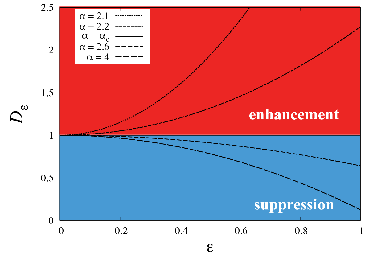
Unlike the asymptotic behavior of the variance for $\alpha>2$, it depends on the initial ensemble for $1<\alpha<2$. This is due to the fact that the variance of $N_{t}$ is

and

where $D(\alpha)=2c\mu^{-3}/\Gamma(4-\alpha)$. It follows that the variances of the displacement in ordinary and equilibrium renewal processes are given by

and

respectively. Therefore, the spreading of particles with respect to the mean becomes superdiffusive with exponent ($3-\alpha$). However, it should be noted that the coefficients of the leading terms differ by a factor $(\alpha-1)$ according to the initial ensemble. This initial-ensemble dependence is sometimes observed for the case when the second moment of the waiting time diverges [45, 46, 47, *Godec2013a, 49].

For $1<\alpha<2$ and $\Delta\ll t$, the correlation $\langle N_{t}N(t,t+\Delta)\rangle$ is given by

It follows that for the ordinary renewal process the variance of $\delta x(t,t+\Delta)$ with $t\gg\Delta$ becomes

Therefore, the variance of $\delta x(t,t+\Delta)$ for the ordinary renewal process has a clear $t$ dependence and approaches that of the equilibrium renewal process (see Fig. 2). Although the dependence of the variance on the aging time $t$ gradually disappears, i.e., ${\rm Var}(\delta x(t,t+\Delta))_{\rm or}\to{\rm Var}(x(\Delta))_{\rm eq}$ for $t\to\infty$, the aging effect lasts for a long time when $\alpha$ is close to one. This recovery of diffusivity (rejuvenation of diffusivity) is enhanced by the increase of the aging time. In other words, if one waits to start measurements for a long time, the observed diffusivity approaches the diffusivity of the equilibrium initial ensemble, which is enhanced by the factor $(\alpha-1)^{-1}$. This enhancement becomes significant especially for $\alpha\to 1$.

Here, we define the time-averaged variance (TAV) of the displacement as

where we have already observed $\varepsilon\Delta/\mu=\langle\delta x(t^{\prime},t^{\prime}+\Delta)\rangle_{\rm eq}$, which does not depend on $t^{\prime}$. The variable $t$ in Eq. (22) now corresponds to the total measurement time, $\Delta$ is the lag time, and the overline denotes time averaging. Expanding the integrand, the TAV can be written as

As follows from Eqs. (15) and (21), the ensemble average of the TAV converges to a constant for $\alpha>1$,

as $t\to\infty$. In particular, the ensemble average of the TAV for the ordinary renewal process becomes

where $K(\alpha)=\frac{\varepsilon^{2}c\Delta^{2}}{\mu^{3}\Gamma(2-\alpha)}\left(\frac{\mu}{\varepsilon^{2}\Delta}-1\right)$ for $1<\alpha<2$.

The time average of the displacement can be approximated by $\int_{0}^{t-\Delta}\delta x(t^{\prime},t^{\prime}+\Delta)dt^{\prime}/(t-\Delta)\sim\sum_{k=1}^{N_{t}}z_{k}\Delta/t$ for $t\gg\Delta$, where $z_{k}$ is the $k$-th jump ($z_{k}=\pm 1$). By the law of large numbers, i.e., $\sum_{k=1}^{n}z_{k}/n\to\langle z_{k}\rangle=\varepsilon$ for $n\to\infty$, we have

Here, we use a similar approximation for the squared displacements invented in Ref. [50] (see also the argument in Refs. [51, 42, *Schulz2014]). While this approximation is used for the CTRW without bias, it is also valid for the CTRW with bias [51]. Therefore, we have

where $h(\Delta)$ is a function of $\Delta$. For $\alpha>1$ ($\mu<\infty$), the TAV becomes

where $H(\Delta)=\Delta+\varepsilon^{2}h(\Delta)-\frac{2\varepsilon^{2}\Delta^{2}}{\mu}$. Taking the ensemble average of Eq. (28) and using Eq. (24) lead to $h(\Delta)=\frac{\sigma^{2}-\mu^{2}}{\mu^{2}}\Delta+\frac{\Delta^{2}}{\mu}$ and $h(\Delta)=\mu D(\alpha)\Delta^{3-\alpha}-\Delta+\frac{\Delta^{2}}{\mu}$ for $\alpha>2$ and $1<\alpha<2$, respectively. We confirmed numerically that this relation is valid only for $\alpha<2$. For $\alpha>2$, the ensemble average is given by $\langle H(\Delta)\rangle=\Delta+\varepsilon^{2}h(\Delta)-\frac{2\varepsilon^{2}\Delta^{2}}{\mu}$ but an additional term is needed in $H(\Delta)$ and will be considered in detail elsewhere.

To characterize the relaxation process, we consider the relative standard deviation (RSD) [52, *Uneyama2015] of the TAV

This is the squared root of the ergodicity breaking parameter, which is widely used to investigate ergodic properties [51, 54]. For $1<\alpha<2$ using Eq. (28) we have

Therefore, the RSD for $\tau_{0}\ll\Delta\ll t$ becomes

for the equilibrium initial ensemble. For $1<\alpha<2$, the RSD decays as $t^{-\frac{\alpha-1}{2}}$, which is anomalously slower than the usual case, $t^{-\frac{1}{2}}$. Therefore, trajectory-to-trajectory fluctuations of the time-averaged variance remain large even for long measurement times. This slow relaxation has been also discussed in CTRW without bias [55].

The diffusivity for diffusion processes with drift is characterized by the variance of the displacement. Using the paradigmatic CTRW model with drift, we uncovered a novel mechanism of diffusivity enhancement in heterogeneous evironments, which is supported by an increased variance of waiting times. In particular, the diffusivity becomes infinite (superdiffusive) when the variance diverges. In the superdiffusive regime, we found an intrinsic difference of the diffusivity due to the initial ensembles, e.g., for ordinary and equilibrium renewal processes. This initial-ensemble dependence is essential when the second moment of the waiting time diverges. For the ordinary renewal process, the diffusivity increases approaching that of the corresponding equilibrium process according to the increase of the aging time. In other words, if one waits to measure the diffusivity for a long time, the observed diffusivity is greatly enhanced compared to the diffusivity measured immediately. This recovering of diffusivity has a significant implication of rejuvenation in superdiffusive physical systems. We also showed that TAVs converge to a constant, which is given by the ensemble-averaged variance with the equilibrium initial ensemble. Therefore, the system is ergodic whereas there is a distinct dependence of the ensemble-averaged variance on the initial ensemble. Finally, we found that trajectory-to-trajectory fluctuations of the TAVs decay anomalously slow, as compared to standard random walks.

References

- [1] J. B. Knight, A. Vishwanath, J. P. Brody, and R. H. Austin, Phys. Rev. Lett. 80, 3863 (1998).
- [2] T. M. Squires and S. R. Quake, Rev. Mod. Phys. 77, 977 (2005).
- [3] C. Y. Lim, Y. C. Lam, and C. Yang, Biomicrofluidics 4, 014101 (2010).
- [4] W. Feller, An introduction to probability theory and its applications, Vol. 1 (Wiley, New York, 1968).
- [5] P. Reimann, C. Van den Broeck, H. Linke, P. Hänggi, J. M. Rubi, and A. Pérez-Madrid, Phys. Rev. Lett. 87, 010602 (2001).
- [6] P. Reimann, C. Van den Broeck, H. Linke, P. Hänggi, J. M. Rubi, and A. Pérez-Madrid, Phys. Rev. E 65, 031104 (2002).
- [7] M. Evstigneev, O. Zvyagolskaya, S. Bleil, R. Eichhorn, C. Bechinger, and P. Reimann, Phys. Rev. E 77, 041107 (2008).
- [8] P. Reimann and R. Eichhorn, Phys. Rev. Lett. 101, 180601 (2008).
- [9] R. Hayashi, K. Sasaki, S. Nakamura, S. Kudo, Y. Inoue, H. Noji, and K. Hayashi, Phys. Rev. Lett. 114, 248101 (2015).
- [10] X.-G. Ma, P.-Y. Lai, B. J. Ackerson, and P. Tong, Phys. Rev. E 91, 042306 (2015).
- [11] D. Kim, C. Bowman, J. T. Del Bonis-O’Donnell, A. Matzavinos, and D. Stein, Phys. Rev. Lett. 118, 048002 (2017).
- [12] X.-G. Ma, Y. Su, P.-Y. Lai, and P. Tong, Phys. Rev. E 96, 012601 (2017).
- [13] P. Habdas, D. Schaar, A. C. Levitt, and E. R. Weeks, Europhys. Lett. 67, 477 (2004).
- [14] C. Wilhelm, Phys. Rev. Lett. 101, 028101 (2008).
- [15] I. Gazuz, A. M. Puertas, T. Voigtmann, and M. Fuchs, Phys. Rev. Lett. 102, 248302 (2009).
- [16] J. Shin, A. G. Cherstvy, W. K. Kim, and R. Metzler, New Journal of Physics 17, 113008 (2015).
- [17] C. J. Harrer, D. Winter, J. Horbach, M. Fuchs, and T. Voigtmann, J. Phys.: Cond. Matt. 24, 464105 (2012).
- [18] M. Gruber, G. C. Abade, A. M. Puertas, and M. Fuchs, Phys. Rev. E 94, 042602 (2016).
- [19] R. Richert, J. Phys.: Cond. Matt. 14, R703 (2002).
- [20] I. Golding and E. C. Cox, Phys. Rev. Lett. 96, 098102 (2006).
- [21] A. Weigel, B. Simon, M. Tamkun, and D. Krapf, Proc. Natl. Acad. Sci. USA 108, 6438 (2011).
- [22] F. Höfling and T. Franosch, Rep. Prog. Phys. 76, 046602 (2013).
- [23] C. F. E. Schroer and A. Heuer, Phys. Rev. Lett. 110, 067801 (2013).
- [24] O. Bénichou, A. Bodrova, D. Chakraborty, P. Illien, A. Law, C. Mejía-Monasterio, G. Oshanin, and R. Voituriez, Phys. Rev. Lett. 111, 260601 (2013).
- [25] J. F. Reverey, J.-H. Jeon, H. Bao, M. Leippe, R. Metzler, and C. Selhuber-Unkel, Sci. Rep. 5, 11690 (2015).
- [26] G. Gradenigo, E. Bertin, and G. Biroli, Phys. Rev. E 93, 060105 (2016).
- [27] S. Leitmann and T. Franosch, Phys. Rev. Lett. 118, 018001 (2017).
- [28] R. Burioni, G. Gradenigo, A. Sarracino, A. Vezzani, and A. Vulpiani, J. Stat. Mech. , P09022 (2013).
- [29] R. Burioni, G. Gradenigo, A. Sarracino, A. Vezzani, and A. Vulpiani, Commun. Theor. Phys. 62, 514 (2014).
- [30] J.-P. Bouchaud and A. Georges, Phys. Rep. 195, 127 (1990).
- [31] F. Bardou, J.-P. Bouchaud, A. Aspect, and C. Cohen-Tannoudji, Levy statistics and laser cooling: how rare events bring atoms to rest (Cambridge University Press, 2002).
- [32] E. M. Bertin and J.-P. Bouchaud, Phys. Rev. E 67, 026128 (2003).
- [33] S. Burov and E. Barkai, Phys. Rev. Lett. 98, 250601 (2007).
- [34] T. Miyaguchi and T. Akimoto, Phys. Rev. E 83, 031926 (2011).
- [35] T. Miyaguchi and T. Akimoto, Phys. Rev. E 91, 010102 (2015).
- [36] L. Luo and L.-H. Tang, Phys. Rev. E 92, 042137 (2015).
- [37] T. Akimoto, E. Barkai, and K. Saito, Phys. Rev. Lett. 117, 180602 (2016).
- [38] J. Machta, J. Phys. A 18, L531 (1985).
- [39] H. Scher and E. W. Montroll, Phys. Rev. B 12, 2455 (1975).
- [40] D. R. Cox, Renewal theory (Methuen, London, 1962).
- [41] C. Godrèche and J. M. Luck, J. Stat. Phys. 104, 489 (2001).
- [42] J. H. P. Schulz, E. Barkai, and R. Metzler, Phys. Rev. Lett. 110, 020602 (2013).
- [43] J. H. P. Schulz, E. Barkai, and R. Metzler, Phys. Rev. X 4, 011028 (2014).
- [44] E. Barkai, Phys. Rev. E 75, 060104 (2007).
- [45] T. Akimoto and Y. Aizawa, J. Korean Phys. Soc. 50, 254 (2007).
- [46] T. Akimoto, Phys. Rev. Lett. 108, 164101 (2012).
- [47] A. Godec and R. Metzler, Phys. Rev. Lett. 110, 020603 (2013a).
- [48] A. Godec and R. Metzler, Phys. Rev. E 88, 012116 (2013b).
- [49] D. Froemberg and E. Barkai, Phys. Rev. E 87, 030104 (2013).
- [50] T. Miyaguchi and T. Akimoto, Phys. Rev. E 87, 032130 (2013).
- [51] Y. He, S. Burov, R. Metzler, and E. Barkai, Phys. Rev. Lett. 101, 058101 (2008).
- [52] T. Uneyama, T. Akimoto, and T. Miyaguchi, J. Chem. Phys. 137, 114903 (2012).
- [53] T. Uneyama, T. Miyaguchi, and T. Akimoto, Phys. Rev. E 92, 032140 (2015).
- [54] R. Metzler, J.-H. Jeon, A. G. Cherstvy, and E. Barkai, Phys. Chem. Chem. Phys. 16, 24128 (2014).
- [55] T. Akimoto, E. Yamamoto, K. Yasuoka, Y. Hirano, and M. Yasui, Phys. Rev. Lett. 107, 178103 (2011).