Jumping VaR: Order Statistics Volatility Estimator for Jumps Classification and Market Risk Modeling

Starting from the non-parametric threshold estimator introduced in Mancini (2009), we propose an estimator of the integrated variance of jump-diffusion stochastic processes, based on order statistics. As a result, estimates of the process time-varying volatility can be obtained by an iterative method and they can be employed for practical purposes, for example for market risk modeling.
In this section we provide a simple introduction to the estimator, describing the intuition behind it. As a consequence, we intentionally avoided some accuracy in the approach in favour to a better description of the general idea. In the following sections, we provide a formal mathematical description of the statistical estimator we want to introduce.
In a nutshell, we want to obtain a definition of a jump as a realization that is abnormal and anomalous with respect to the other realizations in our time series. For this reason, we need to consider a reference distribution (in the rest of the paper we consider a Gaussian distribution even if the approach can be easily extended to other distributions) and we need to evaluate if a given realization is compatible with it. A typical approach in this case could be to classify as jump (as anomalous realization) all realizations that lie far from the centre of the distribution. A very naive approach could be for example to consider some multiple of the standard deviation of the time series and assume that all the realizations larger (or smaller) than this (negative) threshold are outliers. In our view, this approach is rather rough, as all the realizations above (or below) the (negative) threshold are classified as jumps. On the contrary, it could happen that many realizations do not lie too far from the centre of the distribution, but they are simply too frequent for the reference distribution. A very simple example could be obtained if one considers a T-Student distribution for the realizations and a Gaussian distribution as a reference. As the T-Student distribution has fat tails, once a sufficiently large (in absolute terms) threshold is defined, many realizations will lie below the threshold, even if their frequency is not compatible with a Gaussian distribution. In other words, for a given threshold, only the really extreme realization will be classified as jump, but the tail of the distribution will remain fatter than the one implied by a Gaussian distribution. In any cases, it can be proved that there exists a smart way to define this threshold in order to obtain estimators that satisfy typical statistical convergence requirements Mancini (2009). In this paper we want to develop a different approach that is able to go beyond the truncation effect given by the definition of the threshold while maintaining most of the theoretical framework introduced in Mancini (2009) that represents our main reference. Essentially, the main idea of this paper is based on two key points:

• •

  the mapping of the threshold definition problem into a probability threshold problem

• •

  the introduction of extreme value theory as a statistical tool to identify jumps.

Concerning the first point, we transform the threshold problem in a statistical problem where we want to estimate what is the probability of observing a realization so large (or so small). Even if the two problems are equivalent as we just applied a mapping, we think that this step is relevant from a practical point of view because the definition of a probability threshold is typically easier to understand and to interpret than a threshold on a random variable.
With respect to the second point, we transform the statistical question from what is the probability of observing a realization given a reference distribution? to the question what is the probability of getting a $k-$th maximum as the one observed if we could sample many times a time series of $n$ realizations? By this change in the approach, we are questioning if each ordered realization can be larger (or smaller) than the one observed; in this way, it could happen that the maximum is not large enough to be classified as jump, differently to the $k-$th maximum. In this way, in the above T-Student example, the frequency of largest (smallest) observations can be reduced, avoiding the problem of introducing a truncation of the distribution.
In the following sections, we provide a formal description of these simple ideas with both numerical and empirical examples.

According to the Lévy-Itô Decomposition, a Lévy process is characterized by the superposition of a continuous part, formed by a drift term and a Brownian motion, and independent Poisson processes, possibly infinitely many, as reported in Tankov et al. (2015). Therefore, modeling the stock log-returns as realizations of a Lévy process, we consider the following set-up.

Let $\left\{Y_{t}\right\}_{t\in\mathbbm{R}^{+}}$ be a stochastic process with dynamics

where $W_{t}$ is a standard Brownian motion, $\sigma_{t}$ is the volatility of the continuous part of $Y_{t}$ (named $Y_{t}^{c}$) and $J_{t}$ is a pure jump process.
The pure jump process can have either finite activity (FA), i.e. finitely many “big” jumps can occur in finite time, or infinite activity (IA), i.e. an infinite number of “compensated small” jumps can occur in finite time interval.
Note that we assume the drift term to be negligible and thus we do not include it in the $Y_{t}$ dynamics in Eq. 1.

The quadratic variation of the process $Y_{t}$ corresponds to the sum of the quadratic variation of the continuous part, called integrated variance (IV), and the quadratic variation of the jump component (Tankov et al. (2015)). Formally,

Assuming that the realizations of the $Y_{t}$ process are recorded at $n$ discrete equispaced times $\delta t,\dots,n\delta t=T$, our aim is to estimate the integrated variance of the process disentangling it from the quadratic variation of the jump part.

Naming $Y_{\delta t},Y_{2\delta t},\dots,Y_{(n+1)\delta t}$ the $n+1$ random variables obtained sampling $Y_{t}$ in time, denote by $\Delta_{i}Y:=Y_{\left(i+1\right)\delta t}-Y_{i\delta t}$ for $i=1,\dots,n$ the discrete increments of $Y_{t}$ and, likewise, $\Delta_{i}Y^{c}:=Y_{\left(i+1\right)\delta t}^{c}-Y_{i\delta t}^{c}$ as the discrete increments of the continuous part of $Y_{t}$. The corresponding realizations of such random variables are indicated by lower-case letters, that is $\left\{\Delta_{1}y,\dots,\Delta_{n}y\right\}$, on one hand, and $\left\{\Delta_{1}y^{c},\dots,\Delta_{n}y^{c}\right\}$, on the other hand. This notation will be kept throughout the whole paper.

The non-parametric threshold estimator proposed in Mancini (2009) is defined as

where $\theta\left(\delta t\right)$ is a threshold function that must satisfy $\underset{\delta t\to 0}{\text{lim}}\theta\left(\delta t\right)=0$ and $\underset{\delta t\to 0}{\text{lim}}\frac{\delta t\text{log}\frac{1}{\delta t}}{\theta\left(\delta t\right)}=0$.

The Levy’s Modulus of Continuity Theorem (Sato (1999)) is the key result exploited to prove the consistency of this estimator. It states that

almost surely. Therefore, considering the time grid $0,\delta t,\dots,n\delta t=T$, as enunciated in Mancini (2010) and Mancini (2009),

and, thus, keeping in mind the stochastic integral definition, the absolute value of any path of a stochastic integral with respect to a Brownian motion tends to zero almost surely as the function $\sqrt{2\delta t\text{log}\frac{1}{\delta t}}$. As a result, if $\left(\Delta_{i}Y\right)^{2}>\theta\left(\delta t\right)>2\delta t\text{log}\frac{1}{\delta t}$ then, in the time interval $\delta t$, some jumps in the $Y_{t}$ process must be occurred, when $\delta t$ approaches zeros.

According to Mancini (2009), under the assumptions on the drift, the diffusion and the threshold function stated in the mentioned paper, the threshold estimator is consistent for both cases of finite and infinite activity jump part. Moreover, considering a process with only finite activity jump component and under the same set of hypotheses required for the consistency, the threshold estimator has a Normal asymptotic distribution (i.e. as $\delta t\to 0$, having fixed the grid time horizon $T$) with mean corresponding to the integrated variance and variance proportional to the inverse of the number of time steps at which the realizations of the stochastic process are recorded, fixed the time horizon of the grid. Consequently, the speed of convergence of the estimator to the true parameter depends on the square root of the number of time steps.

The hypotheses on the threshold function are necessary for the consistency of the estimator, although, in practice, we can observe the realizations of $Y_{t}$ only at discrete times and thus the time step $\delta t$ is fixed. Within this setting, the choice of the threshold function is not so easy. For example, the threshold function of the form $\theta\left(\delta t\right):=\left(\delta t\right)^{\beta}$ with $\beta\in\left]0,1\right[$ suggested in Mancini (2009) is dominated by the $2\delta t\text{log}\frac{1}{\delta t}$ only in the limit for $\delta t\to 0$ and thus, if $\delta t$ is sufficiently high, the relation $\left(\Delta_{i}Y\right)^{2}>\theta\left(\delta t\right)>2\delta t\text{log}\frac{1}{\delta t}$ does not hold anymore and some jumps could not be detected by the estimator. In addition, as $\Delta_{i}Y$ depends on the scale parameter $\sigma$, in order to assure that the relation holds, a suitable renormalization procedure must be considered in order to neutralize the effect of the scale parameter.
In accordance with this reasoning, in our implementation of the estimator in Eq. 3, we choose the threshold function exactly equal to

rescaled by the sample variance of $\left\{\Delta_{1}Y,\dots,\Delta_{n}Y\right\}$ (that is proportional to $\delta t$), obtaining a threshold proportional to $\delta t\text{log}\frac{1}{\delta t}$.
It is worth noting that the choice of this threshold function agrees with the results proved in Figueroa-López et al. (2017) concerning the optimal threshold definition by means of the mean square error technique.

Since Eq. 5 holds in the limit, in case of fixed $\delta t$ the following relation must be true

where $\bar{p}\in\left[0,1\right]$ is a certain probability value which refers to the random variable $\underset{i=1,\dots,n}{\text{max}}|W_{\left(i+1\right)\delta t}-W_{i\delta t}|$. Eq. 7 provides a link between the threshold exploited in Mancini (2009) in order to define the estimator reported in Eq. 3 and a probability threshold $\bar{p}$. In particular, by this formulation, the choice of the threshold $\bar{\theta}\left(\delta t\right)$ results into the definition of the confidence level ($\bar{p}$) corresponding to the error in the jump detection that one is willing to accept.

More in general, it is possible to extend this approach for a generic tolerance level $p$ (without considering the absolute value)

for a threshold $\theta^{W}$. Since in our approach, we want to invert Eq. 8 in order to obtain a threshold for a fixed value of the probability $p$, we make explicit this dependence using the notation $\theta^{W}\left(p;n,n\right)$, where the double $n$ refers to the fact that the maximum operator in Eq. 8 can be interpreted as the $n-$th minimum of a sample made by $n$ realizations. This notation will be exploited in the next sections, where we will generalize this setup. In addition, we apply our choice to consider a Gaussian cumulative distribution function (c.d.f.) as a reference distribution, obtaining the following results

where $F_{Z_{n:n}}\left(x\right)=\left(\Phi\left(x\right)\right)^{n}$ is the c.d.f. of the maximum of $n$ Standard Normal random variables and $\Phi\left(x\right)$ is the c.d.f. of a Standard Normal random variable (refer to Appendix A.1 for further details on such derivation). As mentioned in Section 3.1, here we assume that our reference distribution is Normal but the approach can be easily extended to other reference distributions. The notation $Z_{k:j}$ stands for the $k-$th realization over an (increasing) ordered sample of $j$ elements.
It is worth noting that, since the Normal distribution is symmetric, the random variables $Z_{n:n}$ and $-Z_{1:n}$ (where $Z_{1:n}$ is the minimum of $n$ Standard Normal random variables) have the same distribution. In the following, we will consider Eq. 8 as starting point for the definition of our new volatility estimator.

In the light of the approximation stated in Appendix A.2, $\theta\left(p;n,n\right)$ multiplied by the square root of the sample variance of $\left\{\Delta_{1}Y,\dots,\Delta_{n}Y\right\}$ can be set as threshold function to plug-in in Eq. 3 to estimate the IV of the Lévy process $Y_{t}$, once the tolerance level $p$ is fixed (note that here we are assuming that the volatility is constant in time, whereas in the next section we will relax this hypothesis).
This choice implies that all the realizations in the set $\left\{\Delta_{1}y,\dots,\Delta_{n}y\right\}$ larger, in absolute terms, than the maximum value acceptable for the discrete increments of $Y_{t}^{c}$ are excluded from the IV computation.
Nevertheless, this choice does not take into account the possibility of having realizations in the set $\left\{\Delta_{1}y,\dots,\Delta_{n}y\right\}$ which, even being smaller than the maximum acceptable value, are too frequent to be Gaussian and, thus, to be realizations of the discrete increments of $Y_{t}^{c}$ only. According to this reasoning, the threshold $\theta\left(p;n,n\right)$ can be replaced by a realization-varying threshold $\theta\left(p;k,n^{\prime}\right)$, whose value depends on the progressive classification of the ordered realizations of $\left\{\Delta_{1}y,\dots,\Delta_{n}y\right\}$.
More precisely, starting from Eq. 8 and substituting the maximum over the $n$ observations with the $k$-th order statistic in the dataset of size $n^{\prime}$, a more general threshold function $\theta\left(p;k,n^{\prime}\right)$ can be defined. Formally,

where

is the c.d.f. of the $k$-th order statistic in the dataset of $n^{\prime}$ Standard Normal random variables and $I_{x}\left(a,b\right)$ is an Incomplete Beta function with parameters $a,b$. (The whole derivation of the threshold $\theta\left(p;k,n^{\prime}\right)$ is reported in Appendix A.1). Moreover, thanks to the symmetry of the Normal distribution, $Z_{k:n^{\prime}}$ has the same distribution of $-Z_{\left(n^{\prime}-k+1\right):n^{\prime}}$.

Therefore, the procedure can be summarized as follows: $\left\{\Delta_{1}y,\dots,\Delta_{n}y\right\}$ are ordered and the largest observation in this set is compared with the threshold $\theta\left(p;n,n\right)$ rescaled by the square root of the sample variance of $\left\{\Delta_{1}y,\dots,\Delta_{n}y\right\}$; depending on whether the largest observation has been classified as jump or not, the threshold itself can be updated to $\theta\left(p;n-1,n-1\right)$ or $\theta\left(p;n-1,n\right)$, always rescaling by the square root of the sample variance of $\left\{\Delta_{1}y,\dots,\Delta_{n}y\right\}$. The new threshold so obtained can then be compared with the second largest element in the sample and so on and so forth. The formal definition of such new estimator of the IV based on the order statistics theory is reported hereafter.

First of all, we denote the ordered set of the discrete increments of the $Y_{t}$ process as $\left\{\Delta_{n:n}Y,\dots,\Delta_{1:n}Y\right\}$ with $\Delta_{i:n-1}Y\leqslant\Delta_{\left(i+1\right):n}Y\quad i=1,\dots,n$. Moreover, we introduce the increasing sequences of sets $\left\{\mathcal{G}_{i}\right\}_{i=0}^{m}$ and $\left\{\mathcal{G}^{{}^{\prime}}_{i}\right\}_{i=0}^{m^{\prime}}$, with $m=\left\lceil\frac{n}{2}\right\rceil$ and $m^{\prime}=\left\lfloor\frac{n}{2}\right\rfloor$. Assuming $n$ even for simplicity, we define

where $I_{i}$ and $I^{{}^{\prime}}_{i}$ are random variables progressively defined as

While the threshold function $\tilde{\theta}\left(i,\mathcal{G}_{a},\mathcal{G}_{b}^{{}^{\prime}}\right)$ has the following definition

where $\hat{\sigma}^{2}$ indicates the sample variance estimator of $\left\{\Delta_{1}Y,\dots,\Delta_{n}Y\right\}$ and $\theta\left(p;k,n^{\prime}\right)$ is computed according to the formulas in Eq. 10 and Eq. 11 given $p$.

Fixed a tolerance level $p\in\left[0,1\right]$, the Order Statistic (OS) estimator is defined as follows

It should be noticed that, in the OS estimator formulation, each random variable corresponding to an increment of the process $Y_{t}$ is compared with a suitable threshold that is updated according to the new information flow arrival, while $\hat{\sigma}^{2}$ is used to appropriately rescale the realization-varying threshold.
Basically, the algorithm which updates the information to define the thresholds starts from the maximum observation, then moves to the minimum observation, than removes towards the second largest realization and so on and so forth. The sequences $\left\{\mathcal{G}_{i}\right\}_{i=1}^{m}$ and $\left\{\mathcal{G}^{{}^{\prime}}_{i}\right\}_{i=1}^{m^{\prime}}$ allow to take into account the information history to update the thresholds and the introduction of the second sequence $\left\{\mathcal{G}^{{}^{\prime}}_{i}\right\}_{i=1}^{m^{\prime}}$ has the goal of exploiting the property of symmetry of the Normal distribution in the definition of our new estimator. In the practical use of the estimator, it should be noticed that the observations should be half positive and half negative in order to avoid possible distortion, this is clearly coherent with the symmetric choice of the distribution.

To give an intuition of the behaviour of this new estimator, we propose hereafter a simplified setting. In Figure 1, possible realizations of Standard Normal random variables (blue segments) with their threshold levels (dashed lines) are shown in decreasing order. The third ordered observation is composed by a Gaussian realization with the addition of a small jump realization (red interval). The comparison between the second and the third ordered observations underlines the need for taking into account the frequency of the realizations as well as their sizes, in the jump detection procedure. Indeed, if a fixed threshold, corresponding for example to the maximum admissible value for Normal random variables, having set the tolerance level $p$, was used to discriminate observations contaminated by jumps or not, the third realization of Figure 1 would not be detected as jump. On the contrary, the use of realization-varying thresholds allows to identify this kind of realizations interested by a jump component. Roughly speaking, an unusually high frequency of observations near the second and the third greatest values of the observations is interpreted by our estimator as a signal that these realizations cannot come from a Gaussian random variable. Obviously, our estimator is not able to disentangle which realization is really affected by a jump.
Moreover, for the sake of completeness, pure Gaussian realizations could also be detected as jumps by the OS estimator with a certain probability (whose maximum level is $p\%$).

This estimator is practically implemented by the simple iterative algorithm reported in Algorithm 1. For simplicity, as already stated, we consider the case of an even number of $n$ observations.

A further extension concerning the OS estimator is its application to an iterative algorithm in order to estimate the time-varying volatility of the $Y_{t}$ process.

The estimation of the local volatility $\sigma_{t}$ of the $Y_{t}$ process is not completely straightforward and it involves an iterative two-step estimation procedure. At first, the process realizations must be renormalized by the corresponding local volatility estimates and, then, the OS estimator, including a kernel function, must be applied to such renormalized observation set, obtaining new time-varying volatility estimates. The formal definition is the following.

First of all, a kernel function with bandwidth $h$ is defined as

where $K\left(s\right)$ is a non-negative weighting function, i.e. such that $\int_{-\infty}^{+\infty}K\left(s\right)\mathrm{d}s=1$ and $K\left(s\right)\geqslant 0\quad\forall s$.

Considering the iteration $j>1$ and let $\left\{s_{i}^{\left(j\right)}\right\}_{i=1}^{n}$ be the $j$-th sequence of local volatility estimates associated to the record time of each random variable in the set $\left\{\Delta_{1}Y,\dots,\Delta_{n}Y\right\}$, then we consider the $j$-th set of renormalized random variables

Once named $\left\{\Delta_{n:n}\bar{Y}^{\left(j\right)},\dots,\Delta_{1:n}\bar{Y}^{\left(j\right)}\right\}$ the ordered set of these variables, we introduce the function $f^{\left(j\right)}$ that maps the index $i$ of each random variable in the ordered set $\left\{\Delta_{\left(n-i+1\right):n}\bar{Y}^{\left(j\right)}\right\}_{i=1}^{n}$ to the index $\tilde{i}=f^{\left(j\right)}\left(i\right)$ of the corresponding random variable in the set $\left\{\Delta_{i}\bar{Y}^{\left(j\right)}\right\}_{i=1}^{n}$.
The kernel OS estimator, for the $j$-th iteration, is defined as

where the sequences $\left\{\bar{\mathcal{G}}^{\left(j\right)}_{i}\right\}_{i=0}^{m}$ and $\left\{\bar{\mathcal{G}}^{{}^{\prime}\left(j\right)}_{i}\right\}_{i=0}^{m^{\prime}}$ are such that

and $\bar{I}^{\left(j\right)}_{i}$ and $\bar{I}^{{}^{\prime}\left(j\right)}_{i}$ are random variables progressively defined as

with $\bar{X}^{\left(j-1\right)}_{k}:=\left\{\begin{array}[]{ll}\bar{I}^{\left(j-1\right)}_{n-f^{\left(j-1\right)^{-1}}\left(f^{\left(j\right)}\left(k\right)\right)+1}&\text{if }f^{\left(j-1\right)^{-1}}\left(f^{\left(j\right)}\left(k\right)\right)\in\left\{n,\dots,\left\lceil\frac{n}{2}\right\rceil\right\}\\ \bar{I}^{{}^{\prime}\left(j-1\right)}_{f^{\left(j-1\right)^{-1}}\left(f^{\left(j\right)}\left(k\right)\right)}&\text{if }f^{\left(j-1\right)^{-1}}\left(f^{\left(j\right)}\left(k\right)\right)\in\left\{0,\dots,\left\lfloor\frac{n}{2}\right\rfloor\right\}\end{array}\right.$ and $m,m^{\prime}$ as specified in Subsection 3.5.
The threshold function $\bar{\theta}\left(i,\bar{\mathcal{G}}_{a}^{\left(j\right)},\bar{\mathcal{G}}_{b}^{{}^{\prime}\left(j\right)}\right)$ writes as

and the kernel weight $K_{h,\tilde{i}}^{t}:=K_{h}\left(\tilde{i}\delta t-t\right)$ is the kernel value associated with the order statistic $\Delta_{i:n}\bar{Y}$.

Note that $f^{\left(j-1\right)^{-1}}\left(f^{\left(j\right)}\left(i\right)\right)$ stands for the index of the ordered random variable of $\left(j-1\right)$-th iteration corresponding to the ordered random variable with index $i$ of the $j$-th iteration. The variables $\bar{X}^{\left(j-1\right)}_{k}\;k=1,\dots,n$ allow to take into account the observations that have already been detected as jumps in the previous iterations of the algorithm in order to exclude them from the volatility estimation of the current iteration.
Furthermore, the inclusion of kernel weights in the definition of this estimator allows to give different importance to the observations in the sample in accordance with their temporal proximity to the time instant at which the local volatility needs to be estimated.

In addition, once ${\hat{\sigma}^{2\hskip 8.19447pt\left(j\right)}}_{OS}\left(t\right)$ has been computed for all $t\in\left\{0,\delta t,\dots,n\delta t=T\right\}$, the set $\left\{s_{i}^{\left(j-1\right)}\right\}_{i=1}^{n}$ can be updated with these new estimates and the estimator can be applied again to the new renormalized random variables.

As starting volatility estimates, the sample variance of the whole set $\left\{\Delta_{1}Y,\dots,\Delta_{n}Y\right\}$ can be coupled to each random variable $\Delta_{i}Y$ for $i=1,\dots,n$.
It is worth mentioning that, with respect to the first iteration ($j=1$), the indicators $\bar{I}_{i}^{\left(1\right)}$ and $\bar{I}_{i}^{{}^{\prime}\left(1\right)}$ are defined as

and $\bar{X}^{\left(0\right)}_{i}=0\quad\forall i=1,\dots,n$. All the other variables and parameters coincide with the ones previously stated.

Finally, it is worth noting that, in general, the kernel function is an even function (i.e. $K\left(s\right)=K\left(-s\right)$), nevertheless, in order not to use information time preceding the volatility calculation time, in our implementation of such estimator we use a one-sided kernel function, that is $K\left(s\right)\neq 0$ only for $s\leqslant 0$. Thus, without loss of generality, we assume that the kernel function can also be non-symmetrical.
More precisely, the weighting function that we use in our practical implementation of such estimator is $K_{h}\left(t_{i}-t\right)=\left\{\begin{array}[]{ll}\frac{1}{h}&\text{if}\quad|t_{i}-t|\leqslant\left(h+1\right)\delta t\quad\text{and}\quad t_{i}-t<0\\ 0&\text{otherwise}\end{array}\right.$ for each $t_{i}\in\left\{0,\delta t,\dots,n\delta t=T\right\}$.

The iterative algorithm to compute the time-varying volatility of the $Y_{t}$ process is reported in Algorithm 2.

An on-line version (in Python code) of such algorithm is also available on the website²² 2 https://github.com/sigmaquadro/VolatilityEstimator.

By some approximations, we establish a correspondence between the threshold estimator proposed in Eq. 3 and the OS estimator defined in Eq. 15. For practical purposes, this match can be employed to perform a fair comparison between these two estimators.

In detail, starting from the OS estimator defined in Eq. 15 and fixing the threshold level equal to $\tilde{\theta}\left(i,\mathcal{G}_{a},\mathcal{G}^{{}^{\prime}}_{b}\right)\equiv\tilde{\theta}=\sqrt{\hat{\sigma}^{2}}\theta\left(\bar{p};n,n\right)$ for all $i=1,\dots,n$, we get that each observation in the sample $\left\{\Delta_{1}y,\dots,\Delta_{n}y\right\}$ is compared with the maximum admissible value for the discrete increments of $Y_{t}^{c}$, having set the tolerance level $\bar{p}$.
This particular implementation of the OS estimator is comparable to the threshold estimator in Eq. 3 with threshold function corresponding to $\theta\left(\delta t\right)=2\text{log}\frac{1}{\delta t}\hat{\sigma}^{2}$ with $\delta t$ chosen such that

where $Z_{i}=\frac{W_{\left(i+1\right)\delta t}-W_{i\delta t}}{\sqrt{\delta t}}\sim N\left(0,1\right)\quad\forall i=1,\dots,n$. The approximation holds for large $\sqrt{2\text{log}\frac{1}{\delta t}}$ and its derivation is reported in Appendix A.2.
We use this correspondence between the two estimators in order to be able to produce their fair performance comparison in the simulation tests.

Moreover, employing a different c.d.f. in the order statistic computation involved in the OS estimator represents a further extension of such estimator.
Indeed, as previously mentioned, recognizing that all the formulas proposed in Subsection 3.5 hold substituting the c.d.f. of the Standard Normal random variable with a symmetric distribution, the OS estimator can be implemented also assuming that the increments of the continuous part of $Y_{t}$ have a distribution different from the Normal one but still symmetric. For instance, assuming that their distribution is the t-Student one.
Obviously, this is just an observation and additional comments and details are not included in this paper.

We evaluated the performances of the OS estimator by applying it on simulated samples coming from stochastic processes with either finite activity or infinite activity jump part.
More precisely, we simulated two different processes: the Merton process, having a jump part corresponding to a compounded Poisson Process (finite activity), and a process composed by the superposition of a Brownian motion and an independent Variance-Gamma (VG) process, having infinite activity jump part.

For all tests, we also compared the results concerning the jump detection obtained by the OS estimator with the ones produced by the threshold estimator. As previously explained, in order to make a fair comparison of these two estimators, we implemented the threshold estimator with threshold function stated in Subsection 3.7 and with $\delta t$ calibrated in accordance with Eq. 23.
In practice, as far as the OS estimator is concerned, we used the iterative algorithm proposed in Subsection 3.6, while, with respect to the threshold estimator, we properly adapted the considered algorithm to the threshold estimator and we applied it.

We considered the following Merton model dynamics

where $W_{t}$ is a standard Brownian motion, $\sigma$ is the volatility of the continuous part, $N_{t}$ is a Poisson process with constant intensity $\lambda$ and, conditionally on a jump occurring, $\gamma$ is the jump size $\sim N\left(\mu,\delta^{2}\right)$ with mean $\mu$ and variance $\delta^{2}$. $W_{t}$ and $N_{t}$ are independent.
Chosen a parameter set (reported in the caption of the Figure 2 and 3), we simulated $M=1000$ trajectories of such process and computed the relative increments, $\Delta X_{t}$, in order to estimate the volatility $\sigma$ for each path. We applied both the OS estimator and the threshold estimator to the increment time series and recorded the size of the realizations detected as jumps. As an example, Figures 2(a) and 2(b) show a Merton model trajectory and its increments, respectively. The corresponding jump detections performed by the OS estimator and the threshold estimator are reported in Figures 3(a) and 3(b), respectively. The red dots stand for the realizations identified as jumps by the applied estimator.

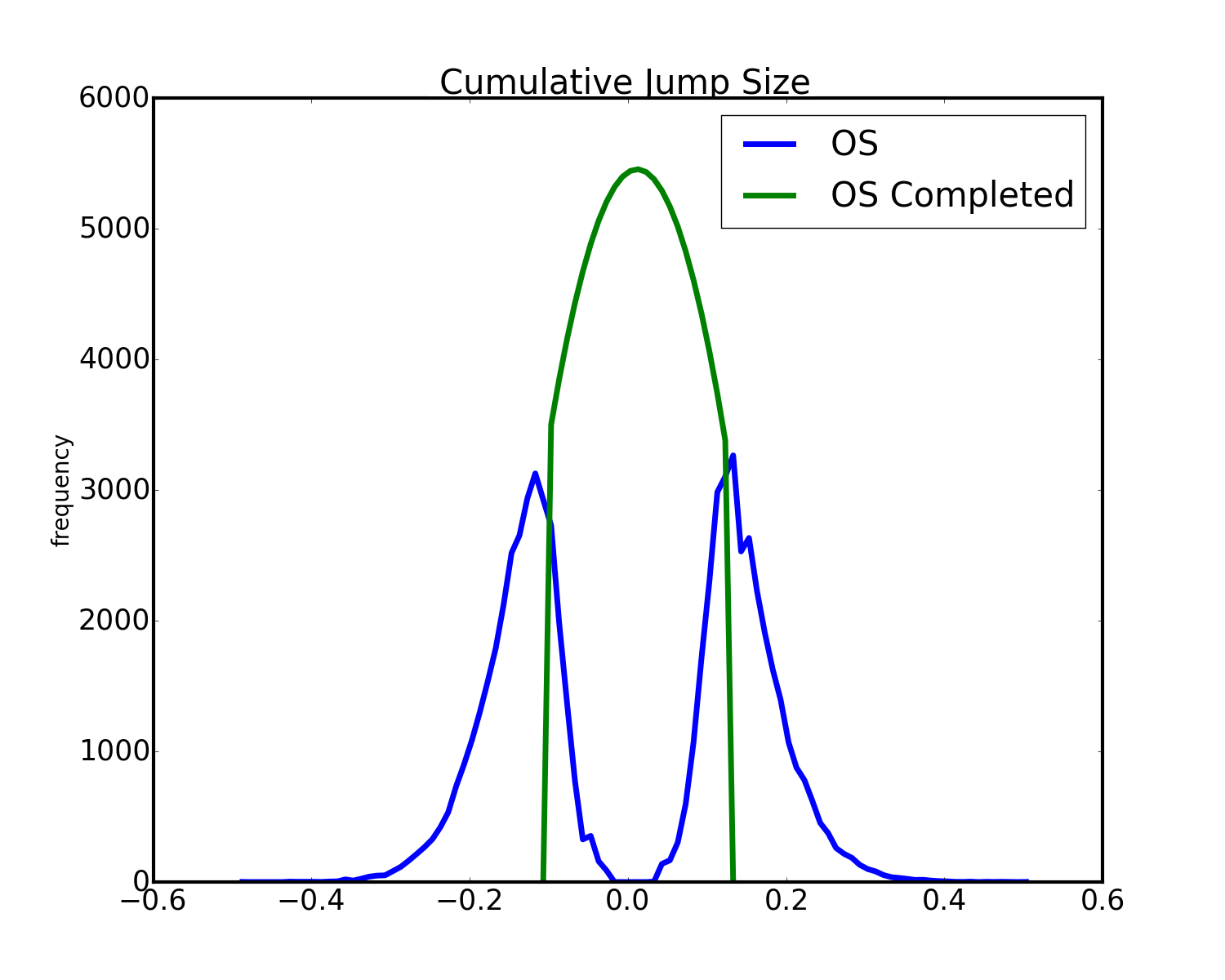
Figure 4(a) shows the convoluted ( i.e. including both the Brownian Motion and the pure jump realizations) jump size frequency distribution recreated from the simulated data provided by the two estimators considering all the samples. The peak in the OS cumulative jump size histogram is due to the error (of type I) in the jump detection that one is willing to accept fixing the tolerance level $p$. This behaviour is confirmed by the comparison between Figure 4(a) and Figure 4(b) where we show the convoluted jump size histogram obtained by applying the OS estimator to the same simulations cleaned-out from the Compounded Poisson process contributions. More precisely, in case of the application of the OS estimator on a rescaled Brownian motion increment time series, the error in the jump detection occurs in the $p\%$ of cases with respect to the maximum (or the minimum, depending on the starting point, i.e. the maximum or the minimum of the ordered realizations, of the recursive algorithm in proposed in Subsection 3.6). In Figure 5 we report the observed probability when applying the OS estimator to a Gaussian noise. Contrarily to our expectations, the probability is not stuck and equal to $p$, but it decreases moving into the central region of the order statistics. This effect is essentially due to the fact that we are neglecting the correlation among ordered realizations when we compute Eq. 11. Despite this decrease of the probability, a peak around 0 is evident in Figure 4 and it is due to the higher probability of observing a realization around zero. As a consequence, even if the probability of committing an error of type I in the jump detection is smaller around zero, the number of misclassified realizations is quite high and this explains the presence of the peak.
To control this error, all realizations identified as jumps by the estimator that are smaller, in absolute value, than the estimated volatility were reclassified as ordinary observations. The new convoluted jump size histogram is presented in Figure 6. Such figure shows the threshold estimator limit in recognizing as non-Brownian realizations many jumps whose size is comparable with the one of the continuous part process increments (hidden jumps), while it shows as the OS estimator, based on order statistics, tries to reduce this bias. The area between the red and blue line represents the gain in the hidden jump identification produced by the OS estimator.

Moreover, starting from the empirical characteristic function (e.c.f.) of the cumulative jump size, we isolated the distribution of the pure jump size to provide a deeper comparison between the two estimator results. Figure 7 reports the obtained distributions and confirms the improvement produced by the OS estimator in the jump detection. The technique used to filter and isolate the jump size distribution from its convolution with the Gaussian distribution is described in Appendix B.1.

Finally, mean time-varying volatility estimates produced by the two estimators, obtained by averaging across the $M$ simulations, are reported in Figure 8. As expected, the OS estimator produces volatility estimates nearer to the real volatility values, since it is capable of detecting jumps even when their size is comparable to the one of the realizations of the continuous part of the process.

For what concerns the infinite activity, the process composed by the sum of a Brownian motion and a VG process (VG+BM process) has the following dynamics

References

- Ait-Sahalia (2004) Yacine Ait-Sahalia. Disentangling diffusion from jumps. Journal of Financial Economics 74(3), 487–528.
- Anderson et al. (1954) T. W. Anderson and D. A. Darling. A Test of Goodness of Fit. Journal of the American Statistical Association 49(268), 765–769. ISSN: 01621459. URL: http://www.jstor.org/stable/2281537.
- Banking Supervision (2012) Basel Committee on Banking Supervision. Fundamental review of the trading book, consultative document. URL: www.bis.org/publ/bcbs219.htm.
- Banking Supervision (2013) Basel Committee on Banking Supervision. Fundamental review of the trading book: A revised market risk framework, consultative document. URL: www.bis.org/publ/bcbs265.htm.
- Banking Supervision (2014) Basel Committee on Banking Supervision. Fundamental review of the trading book: Outstanding issues, consultative document. URL: www.bis.org/bcbs/publ/d305.htm.
- Barndorff-Nielsen et al. (2006) Ole E. Barndorff-Nielsen, Neil Shephard and Matthias Winkel. Limit theorems for multipower variation in the presence of jumps. Stochastic Processes and their Applications 116(5), 796–806.
- Bouchaud et al. (2000) J.P. Bouchaud and M. Potters. Theory of Financial Risks: From Statistical Physics to Risk Management. Aléa Saclay collection. Cambridge University Press, 2000. ISBN: 9780521782326. URL: https://books.google.it/books?id=W3ANngEACAAJ.
- Carr et al. (2002) Peter Carr and Helyette Geman. The Fine Structure of Asset Returns: An Empirical Investigation. The Journal of Business 75(2), 305–332.
- Chen (2010) Fen-Ying Chen. VaR: Exchange Rate Risk and Jump Risk. Journal of Probability and Statistics 2010(Article ID 196461).
- David et al. (2003) H. A. David and H. N. Nagaraja. Order statistics. 3rd ed. Wiley Series in Probability and Statistics. John Wiley, 2003. ISBN: 9780471389262,0-471-38926-9. URL: http://gen.lib.rus.ec/book/index.php?md5=276A8FB1A79A3E37D97A1E47E4BEDED4.
- Figueroa-López et al. (2017) José Figueroa-López and Cecilia Mancini. Optimum thresholding using mean and conditional mean square error. Working Papers - Mathematical Economics 2017-01. Universita’ degli Studi di Firenze, Dipartimento di Scienze per l’Economia e l’Impresa, 2017. URL: http://EconPapers.repec.org/RePEc:flo:wpaper:2017-01.
- Geman (2002) Helyette Geman. Pure jump Levy processes for asset price modelling. Journal of Banking & Finance 26(7), 1297–1316.
- Gibson (2001) Michael S. Gibson. Incorporating event risk into value-at-risk. Finance and Economics Discussion Series 2001-17. Board of Governors of the Federal Reserve System (U.S.), 2001.
- Guan et al. (2004) Lim Kian Guan, Liu Xiaoqing, and Tsui Kai Chong. Asymptotic dynamics and value-at-risk of large diversified portfolios in a jump-diffusion market. Quantitative Finance 4(2), 129–139.
- Mancini (2009) Cecilia Mancini. Non-parametric Threshold Estimation for Models with Stochastic Diffusion Coefficient and Jumps. Scandinavian Journal of Statistics 36(2), 270–296.
- Mancini (2010) Cecilia Mancini. Speed of convergence of the threshold estimator of integrated variance. Working Papers - Mathematical Economics 2010-03. Universita’ degli Studi di Firenze, Dipartimento di Scienze per l’Economia e l’Impresa, 2010. URL: http://EconPapers.repec.org/RePEc:flo:wpaper:2010-03.
- Mancini et al. (2011) Cecilia Mancini and Roberto Renò. Threshold estimation of Markov models with jumps and interest rate modeling. Journal of Econometrics 160(1), 77–92. URL: http://EconPapers.repec.org/RePEc:eee:econom:v:160:y:2011:i:1:p:77-92.
- Pan et al. (2001) Jun Pan and Darrell Duffie. Analytical value-at-risk with jumps and credit risk. Finance and Stochastics 5(2), 155–180.
- Sato (1999) K. Sato. Lévy Processes and Infinitely Divisible Distributions. Cambridge Studies in Advanced Mathematics. Cambridge University Press, 1999. ISBN: 9780521553025. URL: https://books.google.it/books?id=tbZPLquJjSoC.
- Shephard et al. (2003) Neil Shephard and Ole E. Barndorff-Nielsen. Power and bipower variation with stochastic volatility and jumps. Economics Series Working Papers 2003-W18. University of Oxford, Department of Economics, 2003.
- Spadafora et al. (2017) L. Spadafora and G.P. Berman. Theoretical Foundations for Quantitative Finance. World Scientific Publishing Company Pte Limited, 2017. ISBN: 9789813202474. URL: https://books.google.it/books?id=YBMNMQAACAAJ.
- Spadafora (2014) L. Spadafora M. Dubrovich M. Terraneo. Value-at-Risk time scaling for long-term risk estimation. URL: https://arxiv.org/abs/1408.2462.
- Szerszen (2009) Pawel J. Szerszen. Bayesian analysis of stochastic volatility models with Lévy jumps: application to risk analysis. Finance and Economics Discussion Series, 2009-40. Board of Governors of the Federal Reserve System (U.S.), 2009.
- Tankov et al. (2015) P. Tankov and R. Cont. Financial Modelling with Jump Processes, Second Edition. Chapman and Hall/CRC Financial Mathematics Series. Taylor & Francis, 2015. ISBN: 9781420082197. URL: https://books.google.it/books?id=-fZtKgAACAAJ.