Definition and Identification of Information Storage and Processing Capabilities as Possible Markers for Turing-universality in Cellular Automata

Cellular Automata (CA for singular, CAs for plural) are ideal models for physical systems in which space and time are discrete. And elementary cellular automata (ECA for singular, ECAs for plural) is one of the simplest kind of CAs.

ECAs are dynamic systems defined by deterministic rules, working on a 1-dimension list $\{c_{n}\}$ with $n$ cells. Rules can be expressed by function $F$:

where $n\in\mathbb{Z}$.

Therefore, $c_{n}(t+1)$ is the function of itself $c_{n}(t)$ and its two immediate neighbors: $c_{n-1}(t)$ and $c_{n+1}(t)$. Each $c_{n}\left(t\right)$ has two possible states, $0$ or $1$. So there should be a $2^{3}=8$ length list $R$ to define a rule, and there will be $2^{8}=256$ different rules. When $R$ is equal to $\{0,0,0,1,1,1,1,0\}$, by considering it as a binary code, it will equal to $30$ in decimal base, which is the ECA rule 30.

With a given initial list $L_{0}$, an ECA will apply the function $F$ to all cells parallelly to update $L_{t}$ to $L_{t+1}$. i.e.,

By doing this process repeatedly, a matrix $M^{(\text{rule})}=\left(L_{0},L_{1},\ldots,L_{t}\right)$ will be generated, which is the “space–time evolution”. Figure 1 shows two space–time evolutions generated by ECA rule 30 and ECA rule 110, started with the same $L_{0}$.

256 different ECAs can be classified. In this paper, we compare our work with Wolfram’s classification, which are class 1$\sim$4 in [3, 11]. The classes are: 1) Homogeneous; 2) Regular; 3) Chaotic; 4) Complex. Some typical space–time evolutions are shown in Figure 1. There are also some other classifications, see [4, 5, 6].

A particles machine (PM), is a system in which particles can move, collide, annihilate and generate in a homogeneous medium. Figure 2 shows a typical PM. Data and configurations are injected from left in the form of particles, and by executing this system, particles will have interactions. Lines and dotted lines in this figure represent the paths of particles. After time $t$, the system will generate an output. The identity of a particle includes position, phase, and velocity. During collisions, particles can alter their identities, or be generated or annihilated. These changes of particles can be considered as a function of particles that participate in the collision, which is the collision function. Some particles machines are proved to be Turing machines or universal Turing machine (UTM) in [7]. A PM is at least a Turing machine when: 1) Identity of particles can change during collisions; 2) Collision function is depending on identities of particles. For the first requirement, the identity of particles can change during collisions, also means new particles can be generated during collisions. And the second requirement means the result of a collision should depend on types of particles that participate in the collision. If no particles can be generated or annihilated in collisions in a PM, then the PM is not a UTM.

We define a local grid of cells in $M^{(\text{rule})}$ as a particle in ECAs. Here we consider one kind of particles: Their sequence may change periodically or not change through time. We call them “elementary particles”. It will be practical if we start with these simple kind of particles.

Particles contain information, so that information can move in space, and have interaction with other information, which is a kind of computation [9]. All identities of particles: Location, velocity, and sequence, can be computed by collisions. And all of these identities can be preserved if there are no collisions.

To extract particles’ identities from ECAs’ space–time evolutions, a certain sequence should be chosen for the research. We need to choose a sequence as a particle to study, which is the “target particle”. As Figure 3.A shows, we choose target particle $\mathfrak{P}$ at the center-bottom of a space–time evolution and mark the same sequences as “linear particles” $\mathfrak{L}$s, which are the dots in Figure 3.B.

$\mathfrak{P}$ can be explained by the equation $\mathfrak{P}=L_{t_{\text{max}}}(p_{L},p_{R})$, where $L_{t}$ is the $t$–th row of the space–time evolution. $p_{L}$ and $p_{R}$ is the start-index and the end-index for $\mathfrak{P}$.

A particle $P$ at $\left(t;\overrightarrow{x}\right)$, its location may be $\left(t^{\prime};\overrightarrow{x}^{\prime}\right)$ at time $t^{\prime}$ ($t^{\prime}<t$). We call the particle at $\left(t^{\prime};\overrightarrow{x}^{\prime}\right)$ as $P$’s father-particle $P_{f}$. If let $P$ be $\mathfrak{P}$, the $P_{f}$ will be one of the $\mathfrak{L}$s.

All $\mathfrak{L}$s in $P$’s light cone are possible to be the father-particle of $\mathfrak{P}$ (i.e. $\mathfrak{P}_{f}$), we assume that there is one and only one $\mathfrak{L}$ is the $\mathfrak{P}_{f}$, and each $\mathfrak{L}$ has probability $p$ to be the $\mathfrak{P}_{f}$. So when there are $n$ $\mathfrak{L}$s, the probability (i.e. $p_{0}$) for a $\mathfrak{L}_{i}$ to be a father-particle is:

All the $\mathfrak{L}_{i}$ are drawn on a matrix $\mathfrak{M}^{(\text{rule})}$, such as Figure 3.B. $\mathfrak{M}^{(\text{rule})}_{t,x}=p_{0}$ when there is a $\mathfrak{L}$ at $\{t,x\}$, or $\mathfrak{L}_{t,x}=0$. We call $\mathfrak{M}^{(\text{rule})}$ “probability matrix”. The positions with black points will add a number $p_{0}$. Each black point means there is a linear particle $\mathfrak{L}$ of $\mathfrak{P}$ at $\left(t,x\right)$, $(t,x)$ is the location of the black point. $\mathfrak{M}_{t,x}$ equals to $p_{0}\left(p,n\right)$.

The average $\mathfrak{M}^{(\text{rule})}$ that generated with random initial lists:

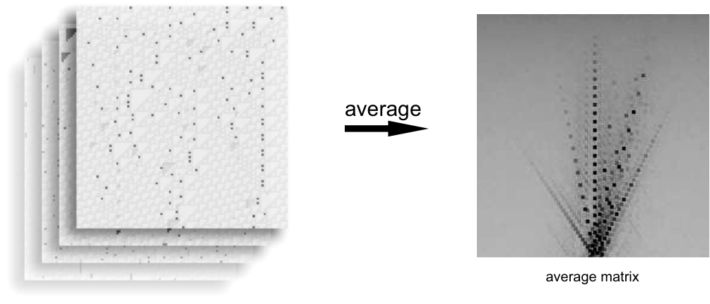
The meaning of an average matrix is, if a particle is found at the center-bottom of a space–time evolution, it may come from position $(t,x)$ with probability $\overline{\mathfrak{M}}_{t,x}/\sum_{t,x}\overline{\mathfrak{M}}_{t.x}$. So the pattern in an average matrix represents traces of particles. We calculate the average matrix with $N=10^{6}$ for each rule.

By observing patterns of average matrices, the identity of particles can be extracted. A typical average matrix is shown in Figure 4. If particles can emerge, there will be some lines in the average matrix. Each line represents at least one particle, and their variations show interactions between particles.

The change of a line’s intensity with time represents interactions between particles. Because if a particle is moving straight without any interactions, the lines’ intensity will not change through time. But if the particle can be generated by other particles, it will not be found before it was created, so that the intensity will change through time, mostly, the intensity will get higher when $t$ is getting higher.

To identify Turing machines and potential UTM, the two parameters we mentioned above will be used to classify ECA rules into four classes. According to the theorem of particle machines [7], when $T(\textrm{rule})\geq 2$ and $C(\textrm{rule})=1$, then this ECA rule behave as a Turing machine and potentially be a UTM. A particle machine that is a Turing machine should have at least $2$ particle traces so that it is possible to have interactions between particles. And traces’ intensity should change, which represents that new particles can be generated during collisions. So all rules can be classified into four classes: A). $T\geq 2$ and $C=1$; B). $T<2$ and $C=1$; C). $T<2$ and $C=0$; D). $T\geq 2$ and $C=0$.

Figure 6 shows the final classification for all rules of elementary cellular automata. Each point represents a rule for an elementary cellular automaton. The $x$-axis is “number of traces”, and $y$-axis represent the existence of information traces’ changes, where $0$ means constant, $1$ means variational. The shape of a point represents its class in Wolfram’s classification.

In class A, rules have complex behaviors, and many particles with plentiful interactions can be found. The information here will be stored and processed. Then they can be considered as a Turing machine with enough complexity and computation ability, which was considered to have connections with Turing universality [8, 14]; In class B, rules will generate some random patterns, particles have too many interactions with the background, so that information traces are dissipated. The information here cannot be stored; In class C, rules will generate continuous or random structures without any complex behavior. Rules in this class do not have particles or have particles but no interactions. In class D, rules will generate some structures that do not have enough interactions, which will not have any complex behavior either. New particles cannot be generated during collisions.

Class C can be divided into two subclasses, as shown in Figure 6, separated by a dotted line. We use “$\text{Rule}_{x}$” to express the subclasses. $\text{C}_{0}$ means the subclass of class C with $T$ equal to $0$. $\text{C}_{1}$ means a subclass of class C with $T$ equal to $1$. In $C_{0}$, rules do not have any particles, the information here cannot be stored or processed. In $C_{1}$, rules have particles but do not have interactions between particles. The information here can only be stored but cannot be processed.

When going through the dark curve in Figure 6 (anticlockwise), the frequency of finding interactions is continually growing. And when the frequency is higher than it in class A, it will generate too much noise, so particles and information will be scattered. When it is lower than the frequency in class A, the number of interactions is not enough to do computation or universal computation, so the behavior is too simple to get complex behaviors.

Some typical rules in these 4 classes show in Table 1. All rules’ classification are shown in Figure 7.

The relation between this classification and Wolfram’s classification was also studied. According to Figure 8, Class $C_{1}$ and $D$ have a strong correlation to a certain Wolfram class, which is Class 2. While class $A$, $B$, and $C_{0}$ contain some different Wolfram classes. Here the reduced entropy is used to measure the relation between the two classifications because the Wolfram classification dose not have an order. The reduced entropy is defined as $h=H/H_{\text{max}}=H/\log n$ where $H_{\text{max}}$ is the maximum that entropy $H$ could be.

References

- [1] Edwin Roger Banks, “Universality in Cellular Automata,” IEEE Annual Symposium (IEEE, 1970), pp. 194–215. doi:10.1109/SWAT.1970.27
- [2] Matthew Cook, “Universality in Elementary Cellular Automata,” Complex Systems, 15(1), 2004 pp. 1–40.
- [3] Stephen Wolfram, A New Kind of Science, Champaign: Wolfram Media Inc, 2002.
- [4] Genaro J. Martinez, “A Note on Elementary Cellular Automata Classification,” Journal of Cellular Automata, 2013 arXiv:1306.5577
- [5] Hector Zenil, and Villarreal-Zapata Elena, “Asymptotic Behavior and Ratios of Complexity in Cellular Automata,” International Journal of Bifurcation and Chaos, 23(09), 2013 pp. 1350159.
- [6] Hector Zenil, “Compression-based Investigation of the Dynamical Properties of Cellular Automata and Other Systems,” arXiv preprint, 2009 arXiv:0910.4042.
- [7] Mariusz H. Jakubowski, Ken Steiglitz, and Richard K. Squier, “When Can Solitons Compute?,” Complex Systems, 10(1), 1996 pp. 1–22.
- [8] Jürgen Riedel, Hector Zenil, “Cross-boundary Behavioural Reprogrammability Reveals Evidence of Pervasive Turing Universality,” arXiv preprint, 2017 arXiv:1510.01671
- [9] Adamatzky, Andrew, and Jérôme Durand-Lose. “Collision-based Computing,” Handbook of Natural Computing, Berlin Heidelberg: Springer, 2012 pp. 1949–1978. “
- [10] John Cocke and Marvin Minsky, “Universality of Tag Systems with ,” Journal of the ACM, 11(1), 1964 pp. 15–20, doi:10.1145/321203.321206
- [11] Stephen Wolfram, “Statistical Mechanics of Cellular Automata,” Review of Modern Physics, 55(3), 1983 pp. 601–644, doi:10.1103/RevModPhys.55.601.
- [12] Paul-Jean Letourneau, “Particle Structures in Elementary Cellular Automaton Rule 146,” Complex Systems, 19(2), 2010 pp. 143.
- [13] Marcelo O. Magnasco, “Chemical Kinetics is Turing Universal,” Physical Review Letters, 78(6), 1997 pp. 1190–1193, doi:10.1103/PhysRevLett.78.1190.
- [14] Hector Zenil, Jürgen Riedel, “Asymptotic Intrinsic Universality and Reprogrammability by Behavioural Emulation,” arXiv preprint, 2016 arXiv:1601.0033.
- [15] Stéphane Perrard, Emmanuel Fort, and Yves Couder, “Wave-Based Turing Machine: Time Reversal and Information Erasing,” Physical Review Letters, 117(9), 2016, doi:10.1103/PhysRevLett.117.094502.
- [16] Daniel M. Harris, Julien Moukhtar, Emmanuel Fort, Yves Couder, and John W. M. Bush, “Wavelike Statistics from Pilot-wave Dynamics in a Circular Corral,” Physical Review E, 88(1), 2013, doi:10.1103/PhysRevE.88.011001.
- [17] Hanno Hildenbrandt, Cladio Carere, and Charlotte K. Hemelrijk, “Self-organized Aerial Displays of Thousands of Starlings: a Model,” Behavioral Ecology, 21(6), 2010 pp. 1349–1359, doi:10.1093/beheco/arq149.
- [18] Takashi Nagatani, “Density Waves in Traffic Flow,” Physical Review E, 61(4), 2000, doi:10.1103/PhysRevE.61.3564.
- [19] Dirk Brockmann and Dirk Helbing, “The Hidden Geometry of Complex, Network-driven Contagion Phenomena,” Science, 342(6164), 2013 pp. 1337–1342, doi:10.1126/science.1245200.
Appendix
.1 Particles in ECAs
I define a local grid of cells in as a particle in ECAs. Backgrounds are also particles, which do not have any interactions with other particles or themselves. According to the definition of particles in ECAs: