跳到论文正文
W Papers独立论文阅读器 arXiv:1803.06846 论文正文 计算阅读时间 · 0%
引用这篇论文根据当前论文元数据生成,正式投稿前建议核对。


License: arXiv.org perpetual non-exclusive license
arXiv:1803.06846v2 [math.NA] 15 Mar 2019

∎

A primal discontinuous Galerkin method with static condensation on very general meshes

Journal: Numerische Mathematik
Alexei Lozinski Affiliation: Laboratoire de Mathématiques de Besançon, CNRS UMR 6623, Univ. Bourgogne Franche-Comté, 16 route de Gray, 25030 Besançon Cedex, France.
Tel.: +33 3 81 66 63 16
Fax: +33 3 81 66 66 23
E-mail: alexei.lozinski@univ-fcomte.fr
Received: date / Accepted: date
Abstract

We propose an efficient variant of a primal Discontinuous Galerkin method with interior penalty for the second order elliptic equations on very general meshes (polytopes with eventually curved boundaries). Efficiency, especially when higher order polynomials are used, is achieved by static condensation, i.e. a local elimination of certain degrees of freedom cell by cell. This alters the original method in a way that preserves the optimal error estimates. Numerical experiments confirm that the solutions produced by the new method are indeed very close to that produced by the classical one.

Keywords: 
Discontinuous Galerkin static condensation polyhedral (polygonal) meshes

1 Introduction

The recent years have seen the emergence (or the revival) of several numerical methods capable to solve approximately elliptic partial differential equations using general polygonal/polyhedral meshes. This is witnessed for example by the book [4]. The methods reviewed in this book (if we restrict our attention only to finite element type methods using piecewise polynomial approximation spaces in one form or another) include interior penalty discontinuous Galerkin (DG) methods [6, 2], hybridizable discontinuous Galerkin (HDG) methods ([8], introduced in [10]), the Virtual Element (VE) method ([21], introduced in [20, 5]), the Hybrid High-Order (HHO) method ([14], introduced in [12, 13]). One can add to this list the weak Galerkin finite element [22], which is similar to HDG. The relations between HHO and HDG methods were exhibited in [9].

Among the above, the primal interior penalty DG methods are the most classical. In the symmetric form, also referred to as SIP – symmetric interior penalty, this method dates back to [24, 3] and is now presented and thoroughly studied in several monographs, for example [19, 11]. It is well suited to the discretization on very general meshes because its approximation space is populated by polynomials of degree, say ≤k\leq k, on each mesh cell without any constraints linking the polynomials on two adjacent cells. It leaves thus a lot of freedom on the choice of the mesh cells which can be not only polytopes but also virtually any geometrical shapes. It is generally admitted however that the SIP method is too expensive especially when higher order polynomials are employed. Indeed, its cost, i.e. the dimension of the approximation space, is the product of the number of mesh cells and the dimension of the space of polynomials of degree ≤k\leq k. The cost on a given mesh is thus proportional to k2k^{2} in 2D (resp. k3k^{3} in 3D). This should be contrasted with the cost of HDG or HHO methods which is proportional to kk in 2D (resp. k2k^{2} in 3D).

The goal of the present article is to modify the SIP method so that its cost is reduced to that of HDG or HHO methods. In doing so, we inspire ourselves from the static condensation procedure for the standard continuous Galerkin (CG) finite element methods. It is indeed well known that the dimension of the approximation space in CG is proportional to k2k^{2} in 2D on a given mesh, but the degrees of freedom interior to each mesh cell can be locally eliminated which leaves a global problem of the size proportional to kk (these numbers are changed to, respectively, k3k^{3} and k2k^{2} in 3D). Although the notion of interior degrees of freedom does not make sense in the DG context, we shall be able to select, on each mesh cell, a subspace of the approximating polynomials that can be used to construct a local approximation through the solution of a local problem. The remaining degrees of freedom will then be used in a global problem. We shall thus achieve a significant reduction of the global problem size in the DG SIP-like method, similarly to that achieved in CG by static condensation. The resulting DG method, which can be refereed to as scSIP (static condensation SIP), will not produce exactly the same approximation as the original SIP method. We shall prove however that these two solutions satisfy the same optimal a priori error bounds in H1H^{1} and L2L^{2} norms. Moreover, they turn out to be very close to each other in our numerical experiments.

We treat here only the diffusion equation with variable, but sufficiently smooth, coefficients. The extension to other problems, such as convection-reaction-diffusion, linear elasticity, Stokes, as well as to other DG variants (IIP, NIP) seems relatively straight-forward. Our assumptions on the mesh allow for cells of general shape, not necessarily the polytopes.

The article is organized as follows: in the next section, we present the idea of our method starting by the description of the governing equations. We the recall the static condensation for the classical CG FEM. Our variants of DG FEM (SIP and scSIP) are first introduced in Subsection 2.2. The convergence proofs are in Section 3. They are done assuming some properties of the discontinuous FE spaces and the underlying mesh. In Section 4, we give an example of the hypotheses on the mesh under which the necessary properties of the FE spaces can be established. Finally, some implementation details and numerical illustrations are presented in Section 5.

2 Description of the problem and static condensation for FEM (CG and DG cases)

We consider the second-order elliptic problem

ℒ​u=f​ in ​Ω,u=g​ on ​∂Ω{\mathcal{L}u}=f\text{ in }\Omega,\quad u=g\text{ on }\partial\Omega (1)

where Ω⊂ℝd\Omega\subset\mathbb{R}^{d}, d=2d=2 or 3, is a bounded Lipschitz domain, f∈L2​(Ω)f\in L^{2}(\Omega) and g∈H1/2​(∂Ω)g\in H^{1/2}(\partial\Omega) are given functions. The differential operator ℒ\mathcal{L} is defined by

ℒu=−∂i(Ai​j(x)∂ju){\mathcal{L}u}=-\partial_{i}(A_{{ij}}(x)\partial_{j}u)

with ∂i\partial_{i} denoting the partial derivative in the direction xix_{i}, i=1,…,di=1,\ldots,d and assuming the summation over i,ji,j. The coefficients Ai​jA_{{ij}} are supposed to form a positive definite matrix A=A⁡(x)A=A(x) for any x∈Ωx\in\Omega which is sufficiently smooth with respect to xx so that

α​|ξ|2≤ξT​A​(x)​ξ≤β​|ξ|2,∀ξ∈ℝd,x∈Ω\alpha|\xi|^{2}\leq\xi^{T}A(x)\xi\leq\beta|\xi|^{2},\hskip 10.00002pt\forall\xi\in\mathbb{R}^{d},x\in\Omega (2)

and

|∇Ai​j(x)|≤M,∀x∈Ω,i,j=1,…,d|\nabla A_{{ij}}(x)|\leq M,\hskip 10.00002pt\forall x\in\Omega,i,j=1,\ldots,d (3)

with some constants β≥α>0\beta\geq\alpha>0, M>0M>0.

2.1 Static condensation for CG FEM

To present our idea, we start by recalling the idea of static condensation, going back to [17], as applied to the usual CG finite element method for problem (1). Let us assume for the moment (in this subsection only) that Ω\Omega is a polygon (polyhedron) and introduce a conforming mesh 𝒯h\mathcal{T}_{h} on Ω\Omega consisting of triangles (tetrahedrons). Assuming for simplicity g=0g=0, the usual continuous ℙk\mathbb{P}_{k} finite element discretization of (1) is then written: find uh∈Whu_{h}\in W_{h} such that

a(uh,vh):=∫ΩA∇uh⋅∇vh=∫Ωfvh,∀vh∈Wha(u_{h},v_{h}):=\int_{\Omega}A\nabla u_{h}\cdot\nabla v_{h}=\int_{\Omega}fv_{h},\quad\forall v_{h}\in W_{h} (4)

where WhW_{h} is the space of continuous piecewise polynomial functions (polynomials of degree ≤k\leq k on each mesh cell T∈𝒯hT\in\mathcal{T}_{h} for some k≥1k\geq 1) vanishing on ∂Ω\partial\Omega. The size of this problem, i.e. the dimension of WhW_{h}, is of order k2k^{2} on a given mesh in 2D (resp. k3k^{3} in 3D). To reduce this cost, one can decompose the space WhW_{h} as follows

Wh=Whl​o​c⊕Wh′W_{h}=W_{h}^{{loc}}\oplus W^{\prime}_{h}

where the subspace Whl​o​cW_{h}^{{loc}} consists of functions of WhW_{h} that vanish on the boundaries of all the mesh cells T∈𝒯hT\in\mathcal{T}_{h}, and Wh′W^{\prime}_{h} is the complement of Whl​o​cW_{h}^{{loc}}, orthogonal with respect to the bilinear form aa. Decomposing uh=uhl​o​c+uh′u_{h}=u_{h}^{{loc}}+u_{h}^{\prime} with uhl​o​c∈Whl​o​cu_{h}^{{loc}}\in W_{h}^{{loc}} and uh′∈Wh′u^{\prime}_{h}\in W_{h}^{\prime} we see that (4) is split into two independent problems

uhl​o​c∈Whl​o​c\displaystyle u_{h}^{{loc}}\in W_{h}^{{loc}} :\displaystyle: a⁡(uhl​o​c,vhl​o​c)\displaystyle a(u_{h}^{{loc}},v_{h}^{{loc}}) =∫Ωf​vhl​o​c,∀vhl​o​c∈Whl​o​c\displaystyle=\int_{\Omega}{fv}^{{loc}}_{h},\hskip 10.00002pt\forall v^{{loc}}_{h}\in W^{{loc}}_{h} (5)
uh′∈Wh′\displaystyle u_{h}^{\prime}\in W_{h}^{\prime} :\displaystyle: a⁡(uh′,vh′)\displaystyle a(u_{h}^{\prime},v_{h}^{\prime}) =∫Ωf​vh′,∀vh′∈Wh′\displaystyle=\int_{\Omega}{fv}^{\prime}_{h},\hskip 10.00002pt\forall v^{\prime}_{h}\in W^{\prime}_{h} (6)

The first problem above is further split into a collection of mutually independent problems on every mesh cell T∈𝒯hT\in\mathcal{T}_{h}:

Find ul​o​c,Th such that ∫TA∇ul​o​c,Th⋅∇vl​o​c,Th=∫Ωfvl​o​c,Th,∀vl​o​c,Th∈Wl​o​c,Th\text{Find }u^{{loc,T}}_{h}\text{ such that }\int_{T}A\nabla u^{{loc,T}}_{h}\cdot\nabla v^{{loc},T}_{h}=\int_{\Omega}{fv}^{{loc},T}_{h},\quad\forall v^{{loc},T}_{h}\in W^{{loc},T}_{h} (7)

where Whl​o​c,TW^{{loc},T}_{h} is the restriction of Whl​o​cW^{{loc}}_{h} on TT, i.e. the set of all polynomials of degree ≤k\leq k vanishing on ∂T\partial T. The cost of solution of these local problems is negligible and we thus get very cheaply uhl​o​c|T=uhl​o​c,Tu^{{loc}}_{h}|_{T}=u^{{loc},T}_{h}. Note also that Problem (7) can be recast as

πT​ℒ​(uhl​o​c|T)=πT​f,∀T∈𝒯h\pi_{T}\mathcal{L}(u^{{loc}}_{h}|_{T})=\pi_{T}f,\hskip 10.00002pt\forall T\in\mathcal{T}_{h} (8)

where πT\pi_{T} is the projection to Whl​o​c,TW^{{loc},T}_{h}, orthogonal in L2​(T)L^{2}(T).

On the other hand, Problem (6) remains global but its size is only proportional to kk in 2D (resp. k2k^{2} in 3D) which is much smaller than that of the original problem (4). Indeed, the degrees of freedom are associated to the standard interpolation points of ℙk\mathbb{P}^{k} finite elements on the edges of the mesh. Note also that a basis for Wh′W_{h}^{\prime} can be constructed solving cheap local problems of the type

πT​ℒ​(vh′|T)=0,∀T∈𝒯h\pi_{T}\mathcal{L}(v_{h}^{\prime}|_{T})=0,\hskip 10.00002pt\forall T\in\mathcal{T}_{h} (9)

with appropriate boundary conditions on ∂T\partial T insuring the continuity of functions in Wh′W_{h}^{\prime}.

2.2 DG FEM: SIP and scSIP methods

We turn now to the main subject of this paper: the DG methods. We now let Ω\Omega be a bounded domain of general shape, and 𝒯h\mathcal{T}_{h} be a splitting of Ω\Omega into a collection of non-overlapping subdomains (again of general shape, the precise definitions and assumptions on the mesh will be given Sections 3 and 4). Let VhV_{h} denote the space of discontinuous piecewise polynomial functions of degree ≤k\leq k on each mesh cell T∈𝒯hT\in\mathcal{T}_{h} for some k≥2k\geq 2:11 1 The usual SIP DG method makes perfect sense also for piecewise linear polynomials (k=1k=1). We restrict ourselves however to k≥2k\geq 2 since the forthcoming modification of the method allowing for the static condensation is pertinent to this case only.

Vh={v∈L2(Ω):v|T∈ℙk(T),∀T∈𝒯h}V_{h}=\{v\in L^{2}(\Omega):v|_{T}\in\mathbb{P}_{k}(T),\forall T\in\mathcal{T}_{h}\} (10)

The SIP (symmetric interior penalty) method is then written as: find uh∈Vhu_{h}\in V_{h} such that

ah​(uh,vh)=Lh​(vh),∀vh∈Vha_{h}(u_{h},v_{h})=L_{h}(v_{h}),\hskip 10.00002pt\forall v_{h}\in V_{h} (11)

with the bilinear form aha_{h} and the linear form LhL_{h} defined by

ah(u,v)=∑T∈𝒯h∫TA∇u⋅∇v−∑E∈ℰh∫E({A∇u⋅n}[v]+{A∇v⋅n}[u])+∑E∈ℰhγhE∫E[u][v]a_{h}(u,v)=\sum_{T\in\mathcal{T}_{h}}\int_{T}A\nabla u\cdot\nabla v-\sum_{E\in\mathcal{E}_{h}}\int_{E}(\{A\nabla u\cdot n\}[v]+\{A\nabla v\cdot n\}[u])\\ +\sum_{E\in\mathcal{E}_{h}}\frac{\gamma}{h_{E}}\int_{E}[u][v] (12)

and

Lh(v)=∑T∈𝒯h∫Tfv+∑E∈ℰhb∫Eg(γhEv−A∇v⋅n)L_{h}(v)=\sum_{T\in\mathcal{T}_{h}}\int_{T}fv+\sum_{E\in\mathcal{E}_{h}^{b}}\int_{E}g\left(\frac{\gamma}{h_{E}}v-A\nabla v\cdot n\right) (13)

where ℰh\mathcal{E}_{h} is the set of all the edges/faces of the mesh, ℰhb⊂ℰh\mathcal{E}_{h}^{b}\subset\mathcal{E}_{h} regroups the edges/faces on the boundary ∂Ω\partial\Omega, nn, [⋅][\cdot] and {⋅}\{\cdot\} denote the unit normal, the jump and the mean over E∈ℰhE\in\mathcal{E}_{h}. More precisely, for any internal facet EE shared by two mesh cells T1ET_{1}^{E} and T2ET_{2}^{E}, we choose nn as the unit vector, normal to EE and looking from T1ET_{1}^{E} to T2ET_{2}^{E}. We then define for any function vv which is H1H^{1} on both T1ET_{1}^{E} and T2ET_{2}^{E} but discontinuous across EE

[v]|E:=v|T1E−v|T2E,{A∇v⋅n}|E:=12A(∇v|T1E+∇v|T2E)⋅n[v]|_{E}:=v|_{T_{1}^{E}}-v|_{T_{2}^{E}},\quad\{A\nabla v\cdot n\}|_{E}:=\frac{1}{2}A\left(\nabla v|_{T_{1}^{E}}+\nabla v|_{T_{2}^{E}}\right)\cdot n

On a boundary edge E∈ℰhbE\in\mathcal{E}_{h}^{b}, nn is the unit normal looking outward Ω\Omega and [v]=v[v]=v, {A∇v⋅n}=A∇v⋅n\{A\nabla v\cdot n\}=A\nabla v\cdot n. The parameter hEh_{E} in (12)–(13) is the local length scale of the mesh near the facet EE which will be properly defined in Lemma 1.22 2 The usual choice hE=diam⁡(E)h_{E}=\diam(E) is not appropriate on general meshes since some of the facets can be of much smaller diameter than that of the adjacent cell. Finally, γ\gamma is the interior penalty parameter which should be chosen sufficiently big.

Unlike the case of continuous finite elements, Problem (11) does not allow directly for a static condensation. However, we can construct a modification of (11) that mimics the characterization of local and global components of the solution by the projectors on local polynomial spaces (8)–(9). These spaces are now defined simply as

Vhl​o​c,T=ℙk−2​(T)V^{{loc},T}_{h}=\mathbb{P}^{k-2}(T)

We also let πT,k−2\pi_{T,k-2} to be the projection to Vhl​o​c,TV^{{loc},T}_{h}, orthogonal in L2​(T)L^{2}(T), and propose the following scheme:

  • •

    Compute uhl​o​c∈Vhu_{h}^{{loc}}\in V_{h} by solving

    πT,k−2​ℒ​(uhl​o​c|T)=πT,k−2​f,∀T∈𝒯h\pi_{T,k-2}\mathcal{L}(u^{{loc}}_{h}|_{T})=\pi_{T,k-2}f,\hskip 10.00002pt\forall T\in\mathcal{T}_{h} (14)

    i.e. find uhl​o​c|T∈ℙk​(T)u^{{loc}}_{h}|_{T}\in\mathbb{P}^{k}(T) on all mesh cells T∈𝒯hT\in\mathcal{T}_{h} such that

    ∫Tℒ⁡(uhl​o​c|T)​qT=∫Tf​qT,∀qT∈ℙk−2​(T)\int_{T}\mathcal{L}(u^{{loc}}_{h}|_{T})q_{T}=\int_{T}fq_{T},\quad\forall q_{T}\in\mathbb{P}^{k-2}(T)
  • •

    Define the subspace of VhV_{h}

    Vh′={vh′∈Vh:πT,k−2ℒ(vh′|T)=0,∀T∈𝒯h}V_{h}^{\prime}=\left\{v_{h}^{\prime}\in V_{h}:\pi_{T,k-2}\mathcal{L}(v_{h}^{\prime}|_{T})=0,\hskip 10.00002pt\forall T\in\mathcal{T}_{h}\right\} (15)

    i.e. the subspace of functions vh′∈Vhv_{h}^{\prime}\in V_{h} such that

    ∫Tℒ⁡(vh′|T)​qT=0,∀qT∈ℙk−2​(T)\int_{T}\mathcal{L}(v^{\prime}_{h}|_{T})q_{T}=0,\quad\forall q_{T}\in\mathbb{P}^{k-2}(T) (16)

    on all mesh cells T∈𝒯hT\in\mathcal{T}_{h}.

  • •

    Compute uh′∈Vh′u_{h}^{\prime}\in V_{h}^{\prime} such that

    ah​(uh′,vh′)=Lh​(vh′)−ah​(uhl​o​c,vh′),∀vh′∈Vh′a_{h}(u_{h}^{\prime},v_{h}^{\prime})=L_{h}(v^{\prime}_{h})-a_{h}(u_{h}^{{loc}},v_{h}^{\prime}),\hskip 10.00002pt\forall v^{\prime}_{h}\in V^{\prime}_{h} (17)
  • •

    Set

    uh=uhl​o​c+uh′.u_{h}=u_{h}^{{loc}}+u_{h}^{\prime}. (18)

We shall show that the local problem (14) admits an infinity of solutions. We can choose any of these solutions on each mesh cell to form uhl​o​cu_{h}^{loc}. Nevertheless, the final result uhu_{h} given by (18) is unique, cf. Lemma 3.

Note that the dimension of the “global” space Vh′V_{h}^{\prime} on a given mesh is of order kk in 2D (k2k^{2} in 3D) so that global problem (17) is much cheaper than (11) for large kk. We have thus asymptotically the same costs for the global problems as for CG FEM with static condensation. There is though a fundamental difference between static condensation approaches in CG and DG cases from the implementation point of view: the basis functions for the global space Wh′W_{h}^{\prime} in the CG case are known a priori, whereas those for the space Vh′V_{h}^{\prime} in the DG case should be constructed as solutions to local problems (16), cf. the discussion of the implementation issues in Subsection 5.1. Note however that one can get rid of problems (16) in the special case of a constant coefficient matrix AA in (1), cf. Remark 1. Indeed, (16) is reduced in this case to ℒ⁡(vh′|T)=Ai​j​∂i∂j(vh′|T)=0\mathcal{L}(v^{\prime}_{h}|_{T})=A_{{ij}}\partial_{i}\partial_{j}(v^{\prime}_{h}|_{T})=0 on any cell T∈𝒯hT\in\mathcal{T}_{h}. The structure of Vh′V^{\prime}_{h} does not thus vary from one cell to another and a basis for Vh′V^{\prime}_{h} can be chosen a priori on all the cells.

The local projection step (14) is not necessarily consistent with the original formulation (11) so that the solution uhu_{h} given by (14)–(18) is different from that of (11). We shall prove however that SIP and scSIP approximations satisfy the same a priori error bounds. Moreover, they turn out to be very close to each other in numerical experiments.

3 Well posedness of SIP and scSIP methods and a priori error estimates

Let us now be more precise about the hypotheses on the mesh. Recall that Ω⊂ℝd\Omega\subset\mathbb{R}^{d}, d=2d=2 or 3, is a Lipschitz bounded domain and 𝒯h\mathcal{T}_{h} is a general (not necessarily polygonal or polyhedral) mesh on Ω\Omega. We mean by this that 𝒯h\mathcal{T}_{h} is a decomposition of Ω\Omega into mutually disjoint cells Ω¯=∪T∈𝒯hT¯\bar{\Omega}=\cup_{T\in\mathcal{T}_{h}}\bar{T} so that each cell TT is a Lipschitz subdomain of Ω\Omega and for every T1,T2∈𝒯hT_{1},T_{2}\in\mathcal{T}_{h} we have either T1=T2T_{1}=T_{2} or T1∩T2=∅T_{1}\cap T_{2}=\varnothing (the cells T1∈𝒯hT_{1}\in\mathcal{T}_{h} are treated here as open sets). We also introduce the sets of internal and boundary edges/faces as respectively

ℰhi\displaystyle\mathcal{E}_{h}^{i} ={E=T1¯∩T2¯​ for some ​T1,T2∈𝒯h}\displaystyle=\{E=\bar{T_{1}}\cap\bar{T_{2}}\text{ for some }T_{1},T_{2}\in\mathcal{T}_{h}\}
ℰhb\displaystyle\mathcal{E}_{h}^{b} ={E=T¯∩∂Ω for some T∈𝒯h}\displaystyle=\{E=\bar{T}\cap\partial\Omega\text{ for some }T\in\mathcal{T}_{h}\}

and denote by ℰh:=ℰhi∩ℰhb\mathcal{E}_{h}:=\mathcal{E}_{h}^{i}\cap\mathcal{E}_{h}^{b} the union of all the edges/faces.

Let BTB_{T}, for any T∈𝒯hT\in\mathcal{T}_{h}, denote the smallest ball containing TT, and BTi​nB_{T}^{in} denote the largest ball inscribed in TT. Set hT=diam⁡(T)h_{T}=\diam(T) and h=maxT∈𝒯h⁡hTh=\max_{T\in\mathcal{T}_{h}}h_{T}. From now on, we assume that mesh 𝒯h\mathcal{T}_{h} is

  • •

    Shape regular: there is a mesh-independent parameter ρ1>1\rho_{1}>1 such that, for all T∈𝒯hT\in\mathcal{T}_{h},

    RT≤ρ1​rTR_{T}\leq\rho_{1}r_{T} (19)

    where rTr_{T} is the radius of BTi​nB_{T}^{in} and RTR_{T} is the radius of BTB_{T}. This also implies hT≤2​ρ1​rTh_{T}\leq 2\rho_{1}r_{T} and RT≤ρ1​hTR_{T}\leq\rho_{1}h_{T}.

Choose an integer k≥2k\geq 2 and recall the discontinuous FE space (10). We assume that VhV_{h} has two following properties (and we shall prove in Section 4 that these properties hold under some additional assumptions on the mesh):

  • •

    Optimal interpolation: there exists an operator Ih:Hk+1​(Ω)→VhI_{h}:H^{k+1}(\Omega)\to V_{h} such that for any v∈Hk+1​(Ω)v\in H^{k+1}(\Omega)

    (∑T∈𝒯h(|v−Ih​v|H1​(T)2+1hT2​‖v−Ih​v‖L2​(T)2+hT2|​v−Ih​v|H2​(T)2CLOSECLOSE\displaystyle\hskip-14.22636pt\left(\sum_{T\in\mathcal{T}_{h}}\left(|v-I_{h}v|^{2}_{H^{1}(T)}+\frac{1}{h^{2}_{T}}\|v-I_{h}v\|^{2}_{L^{2}(T)}+h_{T}^{2}|v-I_{h}v|^{2}_{H^{2}(T)}\right.\right. (20)
    +hT∥∇v−∇Ihv∥L2​(∂T)2+1hT∥v−Ihv||L2​(∂T)2))12≤C(∑T∈𝒯hhT2​k|v|Hk+1​(T))12\displaystyle\left.\left.+h_{T}\|\nabla v-\nabla I_{h}v\|^{2}_{L^{2}(\partial T)}+\frac{1}{h_{T}}\|v-I_{h}v||^{2}_{L^{2}(\partial T)}\right)\right)^{\frac{1}{2}}\leq C\left(\sum_{T\in\mathcal{T}_{h}}h_{T}^{2k}|v|_{H^{k+1}(T)}\right)^{\frac{1}{2}}
  • •

    Inverse inequalities: for any vh∈Vhv_{h}\in V_{h} and any T∈𝒯hT\in\mathcal{T}_{h}

    ‖vh‖L2​(∂T)≤ChT​‖vh‖L2​(T)‖∇vh‖L2​(∂T)≤ChT​‖∇vh‖L2​(T)\|v_{h}\|_{L^{2}(\partial T)}\leq\frac{C}{\sqrt{h_{T}}}\|v_{h}\|_{L^{2}(T)}\qquad\|\nabla v_{h}\|_{L^{2}(\partial T)}\leq\frac{C}{\sqrt{h_{T}}}\|\nabla v_{h}\|_{L^{2}(T)} (21)

    and

    |vh|H2​(T)≤ChT​|vh|H1​(T)|v_{h}|_{H^{2}(T)}\leq\frac{C}{{h_{T}}}|v_{h}|_{H^{1}(T)} (22)

We can now study the well posedness and establish optimal a priori error estimates for the classical SIP method (11).

Lemma 1

Under the above assumptions on the mesh and on VhV_{h}, setting

hE\displaystyle h_{E} =2​(1hT1+1hT2)−1\displaystyle=2\left(\frac{1}{h_{T_{1}}}+\frac{1}{h_{T_{2}}}\right)^{-1} for any E∈ℰhi with E=∂T1∩∂T2,\displaystyle\text{ for any }E\in\mathcal{E}_{h}^{i}\text{ with }E=\partial T_{1}\cap\partial T_{2}, (23)
hE\displaystyle h_{E} =hT\displaystyle=h_{T} for any ​E∈ℰhb​ with ​E=∂T∩∂Ω,\displaystyle\text{ for any }E\in\mathcal{E}_{h}^{b}\text{ with }E=\partial T\cap\partial\Omega,

and choosing γ\gamma large enough, γ≥γ0\gamma\geq\gamma_{0}, the bilinear form aha_{h} defined by (12) is coercive, i.e.

ah(vh,vh)≥c⫴vh⫴2,∀vh∈Vha_{h}(v_{h},v_{h})\geq c\interleave v_{h}\interleave^{2},\quad\forall v_{h}\in V_{h} (24)

with some c>0c>0 and the triple norm defined by

⫴v⫴2=∑T∈𝒯h(|v|H1​(T)2+1hT∥[v]∥L2​(∂T)2)\interleave v\interleave^{2}=\sum_{T\in\mathcal{T}_{h}}\left(|v|^{2}_{H^{1}(T)}+\frac{1}{h_{T}}\|[v]\|^{2}_{L^{2}(\partial T)}\right) (25)

The constants c,γ0c,\gamma_{0} depend only on the parameters in the assumptions on the mesh and on VhV_{h}, as well as on α,β\alpha,\beta in (2).

We skip the proof of this well known result. We stress however that our definitions of the length scale hEh_{E} and of the triple norm (25) may be slightly different from those available in the literature. In particular, we avoid to use the diameter of a facet EE (or any other geometrical information on EE) to define hEh_{E}. This choice enables us to establish straightforwardly the coercivity of aha_{h} with respect to the triple norm, which does not see the separate mesh facets either (only the whole boundaries of the mesh cells are present there). More elaborate choices for the interior penalty parameters are proposed in [6].

Lemma 1 implies that problem (11) of the SIP method is well posed. Moreover, we have the following error estimate, the proof of which is also skipped (actually, it goes along the same lines as that of our forthcoming Theorem 3.2).

Theorem 3.1

Assume that the solution u to (1) is in Hk+1​(Ω)H^{k+1}(\Omega). Under the assumptions of Lemma 1, there exists the unique solution uhu_{h} to (11) and it satisfies

|u−uh|H1​(𝒯h)≤C​hk​|u|Hk+1​(Ω)|u-u_{h}|_{H^{1}(\mathcal{T}_{h})}\leq Ch^{k}|u|_{H^{k+1}(\Omega)}

where H1​(𝒯h)H^{1}(\mathcal{T}_{h}) is the broken H1H^{1} space on the mesh 𝒯h\mathcal{T}_{h} and |⋅|H1​(𝒯h):=(∑T∈𝒯h|⋅|H1​(T)2)12|\cdot|_{H^{1}(\mathcal{T}_{h})}:=\left(\sum_{T\in\mathcal{T}_{h}}|\cdot|^{2}_{H^{1}(T)}\right)^{\frac{1}{2}}. If, moreover, the elliptic regularity property holds for (1), then

‖u−uh‖L2​(Ω)≤C​|u|Hk+1​(Ω)​hk+1\|u-u_{h}\|_{L^{2}(\Omega)}\leq C|u|_{H^{k+1}(\Omega)}h^{k+1}

We turn now to the study of the scSIP method (14)–(17) and start by the following technical lemma.

Lemma 2

There exists h0>0h_{0}>0 such that for all T∈𝒯hT\in\mathcal{T}_{h} with hT≤h0h_{T}\leq h_{0} and for all qT∈ℙk−2​(T)q_{T}\in\mathbb{P}_{k-2}(T) one can find uT∈ℙk​(T)u_{T}\in\mathbb{P}_{k}(T) such that

∫TqT​(ℒ​uT)≥12​‖qT‖L2​(T)2\int_{T}q_{T}({\mathcal{L}u}_{T})\geq\frac{1}{2}\|q_{T}\|_{L^{2}(T)}^{2} (26)

and

|uT|H1​(T)2+1hT​‖uT‖L2​(∂T)2≤C​hT2​‖qT‖L2​(T)2|u_{T}|_{H^{1}(T)}^{2}+\frac{1}{h_{T}}\|u_{T}\|_{L^{2}(\partial T)}^{2}\leq{Ch}_{T}^{2}\|q_{T}\|_{L^{2}(T)}^{2} (27)

The constants h0h_{0} and CC depend only on the regularity of the mesh and on α\alpha, β\beta and MM in (2) and (3). One can put h0=+∞h_{0}=+\infty if the coefficient matrix AA is constant on TT.

Proof

Let χT\chi_{T} be the polynomial of degree 2 vanishing on ∂BTi​n\partial B_{T}^{{in}}, i.e.

χT​(x)=(∑i=1d(xi−xi0)2−rT2)\chi_{T}(x)=\left(\sum_{i=1}^{d}(x_{i}-x^{0}_{i})^{2}-r_{T}^{2}\right)

where x0=(x10,…,xd0)x^{0}=(x^{0}_{1},\ldots,x^{0}_{d}) is the center of BTi​nB_{T}^{{in}} and rTr_{T} is its radius. Set Ai​j0=Ai​j​(x0)A^{0}_{{ij}}=A_{{ij}}(x^{0}) and ℒ0\mathcal{L}^{0}=−∂iAi​j0∂j-\partial_{i}A_{{ij}}^{0}\partial_{j}. Consider the linear map

Q:ℙk−2​(T)→ℙk−2​(T)Q:\mathbb{P}_{k-2}(T)\rightarrow\mathbb{P}_{k-2}(T)

defined by

Q⁡(v)=ℒ0​(χT​v)Q(v)=\mathcal{L}^{0}(\chi_{T}v)

The kernel of QQ is {0}\{0\}. Indeed, if Q⁡(v)=0Q(v)=0 then w:=χT​vw:=\chi_{T}v is the solution to

ℒ0​w=0​ in ​BTi​n,w=0​ on ​∂BTi​n\mathcal{L}^{0}w=0\text{ in }B_{T}^{{in}},\hskip 10.00002ptw=0\text{ on }\partial B_{T}^{{in}}

so that w=0w=0 as a solution to an elliptic problem with vanishing right-hand side and boundary conditions. Since QQ is a linear map on the finite dimensional space ℙk−2​(T)\mathbb{P}_{k-2}(T), this means that QQ is one-to-one.

Take any qT∈ℙk−2​(T)q_{T}\in\mathbb{P}_{k-2}(T) and let uT=χT​vTu_{T}=\chi_{T}v_{T} with vT∈ℙk−2​(T)v_{T}\in\mathbb{P}_{k-2}(T) such that Q⁡(vT)=qTQ(v_{T})=q_{T}. We have thus constructed uT∈ℙk​(T)u_{T}\in\mathbb{P}_{k}(T) such that ℒ0​uT=qT\mathcal{L}^{0}u_{T}=q_{T}. This immediately proves (26) in the case of an operator ℒ=ℒ0\mathcal{L}=\mathcal{L}^{0} with constant coefficients. Moreover, by scaling,

|uT|W2,∞​(BT)+1hT|​uT|W1,∞​(BT)+1hT2​‖uT‖L∞​(BT)≤ChTd/2​‖qT‖L2​(BTi​n)|u_{T}|_{W^{2,\infty}(B_{T})}+\frac{1}{h_{T}}|u_{T}|_{W^{1,\infty}(B_{T})}+\frac{1}{h_{T}^{2}}\|u_{T}\|_{L^{\infty}(B_{T})}\leq\frac{C}{h_{T}^{d/2}}\|q_{T}\|_{L^{2}(B_{T}^{{in}})} (28)

with a constant CC depending only on α\alpha, β\beta and the ratio RT/rTR_{T}/r_{T}. Thus,

|uT|H1​(T)≤|T|1/2​|uT|W1,∞​(BT)≤C​hT​‖qT‖L2​(T)|u_{T}|_{H^{1}(T)}\leq|T|^{1/2}|u_{T}|_{W^{1,\infty}(B_{T})}\leq{Ch}_{T}\|q_{T}\|_{L^{2}(T)}

which proves the estimate in H1​(T)H^{1}(T) norm in (27). Similarly, ‖uT‖L2​(T)≤C​hT2​‖qT‖L2​(T)\|u_{T}\|_{L^{2}(T)}\leq{Ch}_{T}^{2}\|q_{T}\|_{L^{2}(T)} and the estimate in L2​(∂T)L^{2}(\partial T) norm in (27) follows by the trace inverse inequality.

It remains to prove (26) in the case of operator ℒ\mathcal{L} with variable coefficients. To this end, we use the estimates in (28) as follows

∫TqT​ℒ​uT\displaystyle\int_{T}q_{T}{\mathcal{L}u}_{T} =∫TqT​ℒ0​uT+∫TqT​∂i((Ai​j−Ai​j0)​∂juT)\displaystyle=\int_{T}q_{T}\mathcal{L}^{0}u_{T}+\int_{T}q_{T}\partial_{i}((A_{{ij}}-A_{{ij}}^{0})\partial_{j}u_{T})
≥‖qT‖L2​(T)2−‖qT‖L2​(T)​|T|1/2​[maxx∈T⁡|A⁡(x)−A0|​|uT|W2,∞​(T)+maxx∈T⁡|∇A​(x)||uT|W1,∞​(T)]\displaystyle\geq\|q_{T}\|_{L^{2}(T)}^{2}-\|q_{T}\|_{L^{2}(T)}|T|^{1/2}[\max_{x\in T}|A(x)-A_{0}||u_{T}|_{W^{2,\infty}(T)}+\max_{x\in T}|\nabla A(x)||u_{T}|_{W^{1,\infty}(T)}]
≥‖qT‖L2​(T)2−‖qT‖L2​(T)​|T|1/2​hT​maxx∈T​|∇A​(x)|​ChTd/2​‖qT‖L2​(BTi​n)\displaystyle\geq\|q_{T}\|_{L^{2}(T)}^{2}-\|q_{T}\|_{L^{2}(T)}|T|^{1/2}h_{T}\max_{x\in T}|\nabla A(x)|\frac{C}{h_{T}^{d/2}}\|q_{T}\|_{L^{2}(B_{T}^{{in}})}
≥‖qT‖L2​(T)2−C​hT​‖qT‖L2​(T)2≥12​‖qT‖L2​(T)\displaystyle\geq\|q_{T}\|_{L^{2}(T)}^{2}-{Ch}_{T}\|q_{T}\|^{2}_{L^{2}(T)}\geq\frac{1}{2}\|q_{T}\|_{L^{2}(T)}

for sufficiently small hTh_{T}. ∎

Corollary 1

Introduce the bilinear form

bh​(q,v)=∑T∈𝒯hhT2​∫Tq​ℒ​ub_{h}(q,v)=\sum_{T\in\mathcal{T}_{h}}h_{T}^{2}\int_{T}{q\mathcal{L}u}

and the space

Mh={v∈L2(Ω):v|T∈ℙk−2(T),∀T∈𝒯h}M_{h}=\{v\in L^{2}(\Omega):v|_{T}\in\mathbb{P}_{k-2}(T),\forall T\in\mathcal{T}_{h}\}

Equip the space VhV_{h} with the triple norm (25) and the space MhM_{h} with

‖q‖h=(∑T∈𝒯hhT2​‖q‖L2​(T)2)1/2\|q\|_{h}=\left(\sum_{T\in\mathcal{T}_{h}}h_{T}^{2}\|q\|_{L^{2}(T)}^{2}\right)^{1/2}

The bilinear form bhb_{h} satisfies the inf-sup condition

infqh∈Mhsupvh∈Vhbh​(qh,vh)‖qh‖h⫴vh⫴≥δ\inf_{q_{h}\in M_{h}}\sup_{v_{h}\in V_{h}}\frac{b_{h}(q_{h},v_{h})}{\|q_{h}\|_{h}\interleave v_{h}\interleave}\geq\delta (29)

with a mesh-independent constant δ>0\delta>0. Moreover, bhb_{h} is continuous on Mh×VhM_{h}\times V_{h} with a mesh-independent continuity bound.

Proof

Take any qh∈Mhq_{h}\in M_{h}, denote qT=qh|Tq_{T}=q_{h}|_{T}, construct uTu_{T} as in Lemma 2 and introduce uh∈Vhu_{h}\in V_{h} by uh|T=uTu_{h}|_{T}=u_{T} on all T∈𝒯hT\in\mathcal{T}_{h}. This yields using (26) and (27),

bh​(qh,uh)⫴uh⫴≥∑T∈𝒯hhT22​‖qh‖L2​(T)2(∑T∈𝒯hC​hT2​‖qh‖L2​(T)2)1/2=2C​‖qh‖h\frac{b_{h}(q_{h},u_{h})}{\interleave u_{h}\interleave}\geq\frac{\sum_{T\in\mathcal{T}_{h}}\frac{h^{2}_{T}}{2}\|q_{h}\|^{2}_{L^{2}(T)}}{\left(\sum_{T\in\mathcal{T}_{h}}{Ch}^{2}_{T}\|q_{h}\|^{2}_{L^{2}(T)}\right)^{1/2}}=\frac{2}{\sqrt{C}}\|q_{h}\|_{h}

which is equivalent to (29) with δ=2/C\delta=2/\sqrt{C}. Finally, the continuity of bhb_{h} is easily seen from the inverse inequality (22). ∎

Lemma 2 implies that operator πT,k−2​ℒ\pi_{T,k-2}\mathcal{L} appearing in (14) is surjective from ℙk​(T)\mathbb{P}^{k}(T) to ℙk−2​(T)\mathbb{P}^{k-2}(T) so that (14) has indeed a solution at least on sufficiently refined meshes. The existence of a solution to (17) follows from the coercivity of aha_{h}. Thus, scheme (14)–(18) produces some uh∈Vhu_{h}\in V_{h}. In order to establish the error estimates for this uhu_{h}, we reinterpret its definition as a saddle point problem.

Lemma 3

The problem of finding uh∈Vhu_{h}\in V_{h} and ph∈Mhp_{h}\in M_{h} such that

ah​(uh,vh)+bh​(ph,vh)\displaystyle a_{h}(u_{h},v_{h})+b_{h}(p_{h},v_{h}) =Lh​(vh),\displaystyle=L_{h}(v_{h}), ∀vh∈Vh\displaystyle\forall v_{h}\in V_{h} (30)
bh​(qh,uh)\displaystyle b_{h}(q_{h},u_{h}) =∑T∈𝒯hhT2​∫Tf​qh,\displaystyle=\sum_{T\in\mathcal{T}_{h}}h_{T}^{2}\int_{T}fq_{h}, ∀qh∈Mh\displaystyle\forall q_{h}\in M_{h} (31)

has a unique solution. Moreover, uhu_{h} given by (30)–(31) coincides with uhu_{h} given by (14)–(18).33 3 More precisely, all solutions uhu_{h} of (14)–(18) may be accompanied by ph∈Mhp_{h}\in M_{h} so that the resulting couples (uh,ph)(u_{h},p_{h}) also solve (30)–(31). Since the solution to (30)–(31) is unique, the inverse statement is also true: uhu_{h} given by (30)–(31) is also a solution to (14)–(18). This implies that uhu_{h} produced by the scheme (14)–(18) is unique.

Proof

The existence and uniqueness of the solution to (30)–(31) follows from the standard theory of saddle point problems, cf. for example Corollary 4.1 from [16], thanks to the coercivity of aha_{h} (Lemma 1) and to the inf-sup property on bhb_{h} (Corollary 1).

In order to explore its relation with uh=uhl​o​c+uh′u_{h}=u^{loc}_{h}+u^{\prime}_{h} from (14)–(18), we note bh​(qh,uhl​o​c)=∑T∈𝒯hhT2​∫Tf​qhb_{h}(q_{h},u^{loc}_{h})=\sum_{T\in\mathcal{T}_{h}}h_{T}^{2}\int_{T}fq_{h} for all qh∈Mhq_{h}\in M_{h} and bh​(qh,uh′)=0b_{h}(q_{h},u_{h}^{\prime})=0 for all qh∈Mhq_{h}\in M_{h} since uh′∈Vh′u_{h}^{\prime}\in V_{h}^{\prime}. We obtain thus

bh​(qh,uhl​o​c+uh′)=∑T∈𝒯hhT2​∫Tf​qh,∀qh∈Mhb_{h}(q_{h},u_{h}^{loc}+u_{h}^{\prime})=\sum_{T\in\mathcal{T}_{h}}h_{T}^{2}\int_{T}{fq}_{h},\quad\forall q_{h}\in M_{h} (32)

Eq. (17) can be rewritten as

Lh​(vh′)−ah​(uhl​o​c+uh′,vh′)=0,∀vh′∈Vh′L_{h}(v_{h}^{\prime})-a_{h}(u_{h}^{loc}+u_{h}^{\prime},v_{h}^{\prime})=0,\quad\forall v_{h}^{\prime}\in V_{h}^{\prime}

This, together with the fact that Vh′V_{h}^{\prime} is precisely the kernel of the bilinear form bhb_{h}, i.e. Vh′={vh∈Vh:b(qh,vh)=0,∀qh∈Mh}V_{h}^{\prime}=\{v_{h}\in V_{h}:b(q_{h},v_{h})=0,\ \forall q_{h}\in M_{h}\}, means that there exists p~h∈Mh\tilde{p}_{h}\in M_{h} such that

bh​(p~h,vh)=Lh​(vh)−ah​(uhl​o​c+uh′,vh),∀vh∈Vh,b_{h}(\tilde{p}_{h},v_{h})=L_{h}(v_{h})-a_{h}(u_{h}^{loc}+u_{h}^{\prime},v_{h}),\quad\forall v_{h}\in V_{h},

cf. Lemma 4.1 from [16]. The last equation can be rewritten as

ah​(uhl​o​c+uh′,vh)+bh​(p~h,vh)=Lh​(vh),∀vh∈Vh,a_{h}(u_{h}^{loc}+u_{h}^{\prime},v_{h})+b_{h}(\tilde{p}_{h},v_{h})=L_{h}(v_{h}),\quad\forall v_{h}\in V_{h}, (33)

Comparing (33)–(32) on one hand with (30)–(31) on the other hand, we identify uhu_{h} with uhl​o​c+uh′u_{h}^{loc}+u_{h}^{\prime} and php_{h} with p~h\tilde{p}_{h}. ∎

Theorem 3.2

Assume that the solution uu to (1) is in Hk+1​(Ω)H^{k+1}(\Omega). Under the assumptions of Lemma 1 and hh sufficiently small, the scSIP method (14)–(18) produces the unique solution uh∈Vhu_{h}\in V_{h}, which satisfies

|u−uh|H1​(𝒯h)≤C​hk​|u|Hk+1​(Ω)|u-u_{h}|_{H^{1}(\mathcal{T}_{h})}\leq Ch^{k}|u|_{H^{k+1}(\Omega)} (34)

If, moreover, the elliptic regularity property holds for (1), then

‖u−uh‖L2​(Ω)≤C​|u|Hk+1​(Ω)​hk+1\|u-u_{h}\|_{L^{2}(\Omega)}\leq C|u|_{H^{k+1}(\Omega)}h^{k+1} (35)
Proof

We shall use the saddle point reformulation (30)–(31). This discretization is consistent. Indeed setting p=0p=0 we have

ah​(u,vh)+bh​(p,vh)\displaystyle a_{h}(u,v_{h})+b_{h}(p,v_{h}) =Lh​(vh),\displaystyle=L_{h}(v_{h}), ∀vh∈Vh\displaystyle\forall v_{h}\in V_{h}
bh​(qh,u)\displaystyle b_{h}(q_{h},u) =∑T∈𝒯hhT2​∫Tf​qh,\displaystyle=\sum_{T\in\mathcal{T}_{h}}h_{T}^{2}\int_{T}{fq}_{h}, ∀qh∈Mh\displaystyle\forall q_{h}\in M_{h}

Thus, by the standard approximation theory for saddle point problems, cf. for example Proposition 2.36 from [15], recalling the coercivity of aha_{h} (Lemma 1) and the inf-sup property on bhb_{h} (Corollary 1), we get

⫴uh−Ih​u⫴+‖ph‖h\displaystyle\interleave u_{h}-I_{h}u\interleave+\|p_{h}\|_{h} ≤C​sup(vh,qh)∈Vh×Mh⫴vh⫴+‖qh‖h=1(ah​(uh−Ih​u,vh)+bh​(ph,vh)+bh​(qh,uh−Ih​u))\displaystyle\leq C\sup_{\scriptsize{\begin{array}[]{l}(v_{h},q_{h})\in V_{h}\times M_{h}\\ \interleave v_{h}\interleave+\|q_{h}\|_{h}=1\end{array}}}(a_{h}(u_{h}-I_{h}u,v_{h})+b_{h}(p_{h},v_{h})+b_{h}(q_{h},u_{h}-I_{h}u))
=C​sup(vh,qh)∈Vh×Mh⫴vh⫴+‖qh‖h=1(ah​(u−Ih​u,vh)+bh​(qh,u−Ih​u))\displaystyle=C\sup_{\scriptsize{\begin{array}[]{l}(v_{h},q_{h})\in V_{h}\times M_{h}\\ \interleave v_{h}\interleave+\|q_{h}\|_{h}=1\end{array}}}(a_{h}(u-I_{h}u,v_{h})+b_{h}(q_{h},u-I_{h}u))
≤C(⫴u−Ihu⫴a2+∑T∈𝒯hhT2∥ℒ(u−Ihu)∥L2​(T)2)12\displaystyle\leq C\left(\interleave u-I_{h}u\interleave_{a}^{2}+\sum_{T\in\mathcal{T}_{h}}h_{T}^{2}\|\mathcal{L}(u-I_{h}u)\|_{L^{2}(T)}^{2}\right)^{\frac{1}{2}}

with the augmented triple norm ⫴⋅⫴a\interleave\cdot\interleave_{a} defined by

⫴v⫴a2:=⫴v⫴2+∑E∈ℰhhE∥{A∇v⋅n}∥L2​(E)2\interleave v\interleave_{a}^{2}:=\interleave v\interleave^{2}+\sum_{E\in\mathcal{E}_{h}}h_{E}\|\{A\nabla v\cdot n\}\|_{L^{2}(E)}^{2}

Applying the interpolation estimates (20) and the triangle inequality gives

⫴u−Ihu⫴a+∥ph∥h≤Chk|u|Hk+1\interleave u-I_{h}u\interleave_{a}+\|p_{h}\|_{h}\leq Ch^{k}|u|_{H^{k+1}} (36)

This implies in particular (34).

To prove the L2L^{2} error estimate, we consider the auxiliary problem for z∈H2​(Ω)z\in H^{2}(\Omega)

ℒ​z=u−uh​ in ​Ω,z=0​ on ​∂Ω{\mathcal{L}z}=u-u_{h}\text{ in }\Omega,\quad z=0\text{ on }\partial\Omega

Then, for all v∈H1​(𝒯h)v\in H^{1}(\mathcal{T}_{h}) and q∈L2​(Ω)q\in L^{2}(\Omega),

ah​(v,z)+bh​(q,z)=∫Ω(u−uh)​v+∑T∈𝒯hhT2​∫T(u−uh)​qa_{h}(v,z)+b_{h}(q,z)=\int_{\Omega}(u-u_{h})v+\sum_{T\in\mathcal{T}_{h}}h_{T}^{2}\int_{T}(u-u_{h})q

Setting v=u−uhv=u-u_{h} and q=p−phq=p-p_{h} (with p=0p=0) and using Galerkin orthogonality yields

‖u−uh‖L2​(Ω)2+∑T∈𝒯hhT2​∫T(u−uh)​(p−ph)\displaystyle\|u-u_{h}\|_{L^{2}(\Omega)}^{2}+\sum_{T\in\mathcal{T}_{h}}h_{T}^{2}\int_{T}(u-u_{h})(p-p_{h}) =ah​(u−uh,z)+bh​(p−ph,z)\displaystyle=a_{h}(u-u_{h},z)+b_{h}(p-p_{h},z)
=ah​(u−uh,z−zh)+bh​(p−ph,z−zh)\displaystyle=a_{h}(u-u_{h},z-z_{h})+b_{h}(p-p_{h},z-z_{h})

for any zh∈Vhz_{h}\in V_{h}. Thus, taking zh=Ih​zz_{h}=I_{h}z and applying the interpolation estimates,

‖u−uh‖L2​(Ω)2\displaystyle\|u-u_{h}\|_{L^{2}(\Omega)}^{2} ≤|ah​(u−uh,z−zh)|+h​‖p−ph‖h​(∑T∈𝒯h‖ℒ​z−ℒ​zh‖L2​(T)2)1/2\displaystyle\leq|a_{h}(u-u_{h},z-z_{h})|+h\|p-p_{h}\|_{h}\left(\sum_{T\in\mathcal{T}_{h}}\|\mathcal{L}z-\mathcal{L}z_{h}\|_{L^{2}(T)}^{2}\right)^{1/2}
+h​‖p−ph‖h​‖u−uh‖L2​(Ω)\displaystyle\qquad+h\|p-p_{h}\|_{h}\|u-u_{h}\|_{L^{2}(\Omega)}
≤Ch⫴u−Ihu⫴a|z|H2​(Ω)+Ch∥ph∥h(|z|H2​(Ω)+∥u−uh∥L2​(Ω))\displaystyle\leq{Ch}\interleave u-I_{h}u\interleave_{a}|z|_{H^{2}(\Omega)}+{Ch}\|p_{h}\|_{h}(|z|_{H^{2}(\Omega)}+\|u-u_{h}\|_{L^{2}(\Omega)})

Recalling |z|H2​(Ω)≤C​‖u−uh‖L2​(Ω)|z|_{H^{2}(\Omega)}\leq C\|u-u_{h}\|_{L^{2}(\Omega)} and (36) yields (35). ∎

4 An example of assumptions on the mesh that guarantee the interpolation and inverse estimates

In this section, we adopt the following assumptions on the mesh.

M1:

𝒯h\mathcal{T}_{h} is shape regular in the sense (19) with a parameter ρ1>1\rho_{1}>1.

M2:

𝒯h\mathcal{T}_{h} is locally quasi-uniform in the following sense: for any two mesh cells T,T′∈𝒯hT,T^{\prime}\in\mathcal{T}_{h} such that BT′∩BT≠∅B_{T^{\prime}}\cap B_{T}\not=\varnothing there holds

1ρ2​hT′≤hT≤ρ2​hT′\frac{1}{\rho_{2}}h_{T^{\prime}}\leq h_{T}\leq\rho_{2}h_{T^{\prime}}

with a parameter ρ2>1\rho_{2}>1.

M3:

The cell boundaries are not too wiggly: for all T∈𝒯hT\in\mathcal{T}_{h}

|∂T|≤ρ3​hTd−1|\partial T|\leq\rho_{3}h_{T}^{d-1}

with a parameter ρ3>0\rho_{3}>0.

We shall show that these assumptions allow us to construct an interpolation operator IhI_{h} to the discontinuous finite element space (10) for k≥2k\geq 2 and to prove the interpolation error estimate (20) and the inverse estimates (21)–(22).

First of all, the assumptions that the mesh is shape regular and locally quasi-uniform entail the following

Lemma 4

Define, for any x∈ℝdx\in\mathbb{R}^{d},

Nb​a​l​l​(x)=#⁡{T∈𝒯h:x∈BT}N_{{ball}}(x)=\#\{T\in\mathcal{T}_{h}:x\in B_{T}\}

with #\# standing for the “number of”. Under assumptions M1 and M2, there holds

Nb​a​l​l​(x)≤Ni​n​t,∀x∈ℝdN_{{ball}}(x)\leq N_{{int}},\quad\forall x\in\mathbb{R}^{d}

with a constant Ni​n​tN_{{int}} depending only on ρ1\rho_{1} and ρ2\rho_{2}.

Proof

Take any x∈ℝdx\in\mathbb{R}^{d} with Nb​a​l​l​(x)>0N_{{ball}}(x)>0 (otherwise, for xx with Nb​a​l​l​(x)=0N_{{ball}}(x)=0, there is nothing to prove). We now choose arbitrarily T′∈𝒯hT^{\prime}\in\mathcal{T}_{h} such that x∈BT′x\in B_{T^{\prime}}, set hx=hT′h_{x}=h_{T^{\prime}}, and then consider all the mesh cells TT such that x∈BT′x\in B_{T^{\prime}}. By Assumption M2, hT≤ρ2​hxh_{T}\leq\rho_{2}h_{x} for any such TT. Hence, by Assumption M1, RT≤ρ1​ρ2​hxR_{T}\leq\rho_{1}\rho_{2}h_{x}, so that TT is inside the ball BxB_{x} of radius 2​ρ1​ρ2​hx2\rho_{1}\rho_{2}h_{x} centered at xx. Recall that TT contains an inscribed ball of radius rT≥RTρ1≥hT2​ρ1≥hx2​ρ1​ρ2r_{T}\geq\frac{R_{T}}{\rho_{1}}\geq\frac{h_{T}}{2\rho_{1}}\geq\frac{h_{x}}{2\rho_{1}\rho_{2}}. If there are several such cells TT, then their respective inscribed balls BTi​nB_{T}^{in} do not intersect each other and they are all inside BxB_{x}. Thus, their number satisfies the bound

Nb​a​l​l(x)≤|Bx|minT∈𝒯h:x∈BT|BTi​n|≤(2​ρ1​ρ2​hx)d(hx2​ρ1​ρ2)d=(2ρ1ρ2)2​dN_{{ball}}(x)\leq\frac{|B_{x}|}{\min\limits_{T\in\mathcal{T}_{h}:x\in B_{T}}|B_{T}^{in}|}\leq\frac{(2\rho_{1}\rho_{2}h_{x})^{d}}{\left(\frac{h_{x}}{2\rho_{1}\rho_{2}}\right)^{d}}=\left({2\rho_{1}\rho_{2}}\right)^{2d}

as announced.∎

Recall that VhV_{h} is the discontinuous FE space on 𝒯h\mathcal{T}_{h} of degree k≥2k\geq 2, cf. (10).

Lemma 5

(Local interpolation estimate) Take any T∈𝒯hT\in\mathcal{T}_{h}. Let πh\pi_{h} denote the L2​(BT)L^{2}(B_{T})-orthogonal projection to the space of polynomials, i.e. given v∈L2​(BT)v\in L^{2}(B_{T}), vh=πh​vv_{h}=\pi_{h}v is a polynomial of degree ≤k\leq k such that

∫BTvh​φh=∫BTv​φh∀φh∈ℙk​(T)\int_{B_{T}}v_{h}\varphi_{h}=\int_{B_{T}}v\varphi_{h}\hskip 10.00002pt\forall\varphi_{h}\in\mathbb{P}^{k}(T)

Under Assumptions M1 and M3, we have then for any v∈Hk+1​(BT)v\in H^{k+1}(B_{T})

|v−vh|H1​(T)+1hT​‖v−vh‖L2​(T)+hT​|v−vh|H2​(T)+hT​‖∇(v−vh)‖L2​(∂T)+1hT​‖v−vh‖L2​(∂T)≤C​hTk​|v|Hk+1​(BT)|v-v_{h}|_{H^{1}(T)}+\frac{1}{h_{T}}\|v-v_{h}\|_{L^{2}(T)}+h_{T}|v-v_{h}|_{H^{2}(T)}\\ +\sqrt{h_{T}}\|\nabla(v-v_{h})\|_{L^{2}(\partial T)}+\frac{1}{\sqrt{h_{T}}}\|v-v_{h}\|_{L^{2}(\partial T)}\leq Ch_{T}^{k}|v|_{H^{k+1}(B_{T})}

with a constant C>0C>0 depending only on ρ1\rho_{1} and ρ3\rho_{3}.

Proof

Since Hk+1​(BT)H^{k+1}(B_{T}) is embedded into L∞​(BT)L^{\infty}(B_{T}), Deny-Lions lemma together with a scaling argument (cf. Theorem 15.3 from [7]) entail

‖v−vh‖L∞​(BT)≤C​hTk+1−d/2​|v|Hk+1​(BT)\|v-v_{h}\|_{L^{\infty}(B_{T})}\leq Ch_{T}^{k+1-d/2}|v|_{H^{k+1}(B_{T})}

Hence,

‖v−vh‖L2​(T)≤|T|12​‖v−vh‖L∞​(BT)≤C​hTk+1​|v|Hk+1​(BT)\|v-v_{h}\|_{L^{2}(T)}\leq|T|^{\frac{1}{2}}\|v-v_{h}\|_{L^{\infty}(B_{T})}\leq Ch_{T}^{k+1}|v|_{H^{k+1}(B_{T})}

and, in view of the hypothesis |∂T|≤ρ3​hTd−1|\partial T|\leq\rho_{3}h_{T}^{d-1},

‖v−vh‖L2​(∂T)≤(ρ3​hTd−1)12​‖v−vh‖L∞​(BT)≤C​hTk+1/2​|v|Hk+1​(BT)\|v-v_{h}\|_{L^{2}(\partial T)}\leq(\rho_{3}h_{T}^{d-1})^{\frac{1}{2}}\|v-v_{h}\|_{L^{\infty}(B_{T})}\leq Ch_{T}^{k+1/2}|v|_{H^{k+1}(B_{T})}

The estimates for |v−vh|H1​(T)|v-v_{h}|_{H^{1}(T)} and ‖∇v−∇vh‖L2​(∂T)\|\nabla v-\nabla v_{h}\|_{L^{2}(\partial T)} are proven in the same way starting from

‖∇v−∇vh‖L∞​(BT)≤C​hTk−d/2​|v|Hk+1​(BT)\|\nabla v-\nabla v_{h}\|_{L^{\infty}(B_{T})}\leq Ch_{T}^{k-d/2}|v|_{H^{k+1}(B_{T})}

This is valid since Hk+1​(BT)H^{k+1}(B_{T}) is embedded into W1,∞​(BT)W^{1,\infty}(B_{T}) for k≥2k\geq 2.

Finally, the estimate for |v−vh|H2​(T)|v-v_{h}|_{H^{2}(T)} holds thanks to the embedding of Hk+1​(BT)H^{k+1}(B_{T}) into H2​(BT)H^{2}(B_{T}) (k≥1k\geq 1).

∎

Lemma 6

(Global interpolation estimate) Let Ih:Hk+1​(Ω)→VhI_{h}:H^{k+1}(\Omega)\rightarrow V_{h} denote the operator obtained by first extending a function v∈Hk+1​(Ω)v\in H^{k+1}(\Omega) by a function v~∈Hk+1​(ℝd)\tilde{v}\in H^{k+1}(\mathbb{R}^{d}) and then applying the local operator πh\pi_{h} from Lemma 5 to v~\tilde{v} on every T∈𝒯hT\in\mathcal{T}_{h}, i.e. Ih​v|T:=(πh​v~)|TI_{h}v|_{T}:=(\pi_{h}\tilde{v})|_{T} on any T∈𝒯hT\in\mathcal{T}_{h}. Then, under Assumptions M1–M3, (20) holds for any v∈Hk+1​(Ω)v\in H^{k+1}(\Omega)

Proof

First, extension theorem for Sobolev spaces [1] insure that there exists v~∈Hk+1​(ℝd)\tilde{v}\in H^{k+1}(\mathbb{R}^{d}) such that

OPENv~=v​ on ​Ωand‖v~‖Hk+1​(ℝd)≤C​‖v~‖Hk+1​(ΩCLOSE)\tilde{v}=v\text{ on }\Omega\quad\text{and}\quad\|\tilde{v}\|_{H^{k+1}(\mathbb{R}^{d})}\leq C\|\tilde{v}\|_{H^{k+1}(\Omega})

To prove (20), we sum the local interpolation estimates of Lemma 5 over all the mesh cells and then use Assumption M2 and Lemma 4:

∑T∈𝒯h(|v−vh|2H1​(T)+1hT2∥v−vh∥2L2​(T)+hT2|v−vh|2H2​(T)+hT∥∇v−∇vh∥2L2​(∂T)+1hT∥v−vh||2L2​(∂T))≤C∑T∈𝒯hhT2​k∫BT|∇k+1v|2dx≤C∫Ω(maxT∈𝒯h:x∈BThT)2​kNb​a​l​l(x)|∇k+1v|2dx≤C​Ni​n​t​ρ22​k​∑T′∈𝒯hhT′2​k​|v|Hk+1​(T)2\sum_{T\in\mathcal{T}_{h}}\left(|v-v_{h}|^{2}_{H^{1}(T)}+\frac{1}{h^{2}_{T}}\|v-v_{h}\|^{2}_{L^{2}(T)}+h_{T}^{2}|v-v_{h}|^{2}_{H^{2}(T)}+h_{T}\|\nabla v-\nabla v_{h}\|^{2}_{L^{2}(\partial T)}+\frac{1}{h_{T}}\|v-v_{h}||^{2}_{L^{2}(\partial T)}\right)\\ \leq C\sum_{T\in\mathcal{T}_{h}}h_{T}^{2k}\int_{B_{T}}|\nabla^{k+1}v|^{2}{dx}\leq C\int_{{}_{\Omega}}{\color[rgb]{0,0,0}\left(\max\limits_{T\in\mathcal{T}_{h}:x\in B_{T}}h_{T}\right)^{2k}}N_{{ball}}(x)|\nabla^{k+1}v|^{2}{dx}\\ \leq{CN}_{{int}}{\color[rgb]{0,0,0}\rho_{2}^{2k}}\sum_{T^{\prime}\in\mathcal{T}_{h}}h_{T^{\prime}}^{2k}|v|^{2}_{H^{k+1}(T)}

∎

Lemma 7

(Inverse inequalities) Under assumptions M1 and M3, (21) and (22) hold for any vh∈Vhv_{h}\in V_{h} and any T∈𝒯hT\in\mathcal{T}_{h}.

Proof

Both bounds in (21) follow immediately from the following one: for any polynomial qhq_{h} of degree ≤l\leq l one has

‖qh‖L∞​(T)≤ChTd/2​‖qh‖L2​(T)\|q_{h}\|_{L^{\infty}(T)}\leq\frac{C}{h^{d/2}_{T}}\|q_{h}\|_{L^{2}(T)}

with C>0C>0 depending only on ρ1\rho_{1} and ll. This follows in turn from

‖qh‖L∞​(BT)≤ChTd/2​‖qh‖L2​(BTi​n)\|q_{h}\|_{L^{\infty}(B_{T})}\leq\frac{C}{h^{d/2}_{T}}\|q_{h}\|_{L^{2}(B_{T}^{{in}})}

where BTi​nB_{T}^{{in}} is the largest ball inscribed in TT. Scaling the ball BTB_{T} to a ball of radius 1 B1B_{1} and considering all the possible positions of the inscribed ball, the last inequality can be rewritten as

‖qh‖L∞​(B1)≤C​minBi​n⊂B1,Bi​n​ a ball of radius ≥ρ1−1​‖qh‖L2​(BTi​n)\|q_{h}\|_{L^{\infty}(B_{1})}\leq C\min_{B^{{in}}\subset B_{1},B^{{in}}\text{ a ball of radius }\geq\rho_{1}^{-1}}\|q_{h}\|_{L^{2}(B_{T}^{{in}})}

This is valid for any polynomial of degree ll by equivalence of norms.

The remaining inverse inequality (22) can be proven similarly:

|vh|H2​(T)≤C​hTd/2​|vh|W2,∞​(BT)≤C​hTd/2−1​|vh|W1,∞​(BT)≤ChT​|vh|H1​(BTi​n)≤ChT|vh|H1​(T)|v_{h}|_{H^{2}(T)}\leq Ch^{d/2}_{T}|v_{h}|_{W^{2,\infty}(B_{T})}\leq Ch^{d/2-1}_{T}|v_{h}|_{W^{1,\infty}(B_{T})}\leq\frac{C}{h_{T}}|v_{h}|_{H^{1}(B_{T}^{{in}})}\leq\frac{C}{h_{T}}|v_{h}|_{H^{1}(T)}

∎

5 Implementation and numerical results

We shall illustrate the convergence of SIP and scSIP methods on polygonal meshes obtained by agglomerating the cells of a background triangular mesh. Both the mesh construction and the following calculations are done in FreeFEM++ [18]. An example of such a mesh is given in Fig. 1. To construct it, we take a positive integer nn (n=4n=4 in the Figure), let FreeFEM++ to construct a Delaunay triangulation of Ω=(0,1)2\Omega=(0,1)^{2} with 4​n4n boundary nodes on each side of the square, and finally agglomerate the triangles of this mesh into n×nn\times n cells as follows. We start by attributing the triangle containing the point

Oi+j​n=(i−1/2n,j−1/2n),i,j=1,…,nO_{i+jn}=\left(\frac{i-1/2}{n},\frac{j-1/2}{n}\right),\quad i,j=1,\ldots,n (37)

to the cell number i+j​ni+jn. Then, iteratively, we run over all the cells and attach yet unattributed triangles neighboring a triangle from a cell to the same cell, until all the triangles are attributed.

Refer to caption Refer to caption

Figure 1: On the left, a polygonal mesh consisting of 4×44\times 4 cells, which are obtained by the agglomeration of the triangles of a finer mesh seen on the right.

Some details of our implementations are given below, followed by the numerical results on two test cases.

5.1 Implementation of SIP ans scSIP methods

Let us enumerate the mesh cells as {T1,…,TNe}\{T_{1},\ldots,T_{N_{e}}\} and introduce a basis {ϕi(l)}i=1,…,Nk\{\phi^{(l)}_{i}\}_{i=1,\ldots,N_{k}} of ℙk​(Tl)\mathbb{P}_{k}(T_{l}) on every cell TlT_{l}. Here and below, NeN_{e} is the number of cells in 𝒯h\mathcal{T}_{h} and NkN_{k} denotes the dimension of ℙk\mathbb{P}_{k}. In our implementation, we form the basis out of monomials shifted to the “center” Ol=(Ol,x,Ol,y)O_{l}=(O_{l,x},O_{l,y}) of the cell TlT_{l}, cf. (37). i.e.

ϕi(l)​(x,y)=ϕi1​i2(l)​(x,y)=(x−Ol,x)i1​(y−Ol,y)i2\phi^{(l)}_{i}(x,y)=\phi^{(l)}_{i_{1}i_{2}}(x,y)=(x-O_{l,x})^{i_{1}}(y-O_{l,y})^{i_{2}}

regrouping the multi-indexes (i1,i2)(i_{1},i_{2}), 0≤i1≤k0\leq i_{1}\leq k, 0≤i2≤k−i10\leq i_{2}\leq k-i_{1} into a single index ii ranging from 11 to NkN_{k}. We form then the matrices 𝐀(l​m)\mathbf{A}^{(lm)} for every pair of cells TlT_{l} and TmT_{m} sharing some parts of their boundaries. These matrices of size Nk×NkN_{k}\times N_{k} represent the bilinear form aha_{h} in our bases and have the following entries

Ai​j(l​m)=ah​(ϕi(l),ϕj(m))A_{ij}^{(lm)}=a_{h}(\phi_{i}^{(l)},\phi^{(m)}_{j})

We also compute the right-hand side vectors F→(l)∈ℝNk\overrightarrow{F}^{(l)}\in\mathbb{R}^{N_{k}} with Fi(l)=Lh​(ϕi(l))F_{i}^{(l)}=L_{h}(\phi_{i}^{(l)}) on every cell TlT_{l}, put all F→(l)\overrightarrow{F}^{(l)} into a single vector F→\overrightarrow{F} of size ND​O​F=Ne​NkN_{DOF}=N_{e}N_{k}, put the matrices 𝐀(l​m)\mathbf{A}^{(lm)} into the block matrix 𝐀\mathbf{A} of size ND​O​F×ND​O​FN_{DOF}\times N_{DOF}, and finally find U→∈ℝND​O​F\overrightarrow{U}\in\mathbb{R}^{N_{DOF}} as solution to

𝐀​U→=F→\mathbf{A}\overrightarrow{U}=\overrightarrow{F}

The vector U→\overrightarrow{U} represents the numerical solution by the SIP method (11) in the following sense: decomposing U→\overrightarrow{U} into the cell-by-cell components U→(l)={Ui(l)}∈ℝNk\overrightarrow{U}^{(l)}=\{{U}^{(l)}_{i}\}\in\mathbb{R}^{N_{k}}, uhu_{h} in (11) is given on each cell TlT_{l} by uh=∑i=1NkUi(l)​ϕi(l)u_{h}=\sum_{i=1}^{N_{k}}{U}^{(l)}_{i}\phi^{(l)}_{i}.

Turning to the scSIP method, we introduce moreover a basis of ℙk−2​(Tl)\mathbb{P}_{k-2}(T_{l}), {ψi(l)}i=1,…,Nk−2\{\psi^{(l)}_{i}\}_{i=1,\ldots,N_{k-2}}, and form the matrices 𝐁(l)\mathbf{B}^{(l)} of size Nk−2×NkN_{k-2}\times N_{k} on every cell TlT_{l} with the entries

B(l)i​j=∫Tlψ(l)iℒϕ(l)j=∫Tlψ(l)i⋅A∇ϕ(l)j−∫∂Tlψ(l)in⋅A∇ϕ(l)jB^{(l)}_{ij}=\int_{T_{l}}\psi^{(l)}_{i}\mathcal{L}\phi^{(l)}_{j}=\int_{T_{l}}\psi^{(l)}_{i}\cdot A\nabla\phi^{(l)}_{j}-\int_{\partial{T_{l}}}\psi^{(l)}_{i}n\cdot A\nabla\phi^{(l)}_{j}

These matrices will serve to compute the local contributions in (14) as well as to construct a basis of the space Vh′V_{h}^{\prime} in (15). As mentioned earlier, the solution to (14) is not unique and one can propose several ways to compute a solution in practice. In our implementation, we have opted for a solution to (14) solving the following saddle-point problem on every cell TlT_{l}

u→(l)+(𝐁(l))T​p→(l)\displaystyle\overrightarrow{u}^{(l)}+(\mathbf{B}^{(l)})^{T}\overrightarrow{p}^{(l)} =0\displaystyle=0
𝐁(l)​u→(l)\displaystyle\mathbf{B}^{(l)}\overrightarrow{u}^{(l)} =Fψ→(l)\displaystyle=\overrightarrow{F_{\psi}}^{(l)} (38)

with Fψ→(l)={Fψ,i(l)}∈ℝNk−2\overrightarrow{F_{\psi}}^{(l)}=\{F^{(l)}_{\psi,i}\}\in\mathbb{R}^{N_{k-2}}, Fψ,i(l)=∫Tlf​ψi(l)F^{(l)}_{\psi,i}=\int_{T_{l}}f\psi^{(l)}_{i}. The unknowns here are u→(l)∈ℝNk\overrightarrow{u}^{(l)}\in\mathbb{R}^{N_{k}} and p→(l)∈ℝNk−2\overrightarrow{p}^{(l)}\in\mathbb{R}^{N_{k-2}} with u→(l)\overrightarrow{u}^{(l)} representing uhl​o​cu_{h}^{loc} on TlT_{l} in the basis {ϕi(l)}\{\phi_{i}^{(l)}\}. The saddle-point problem above is well posed thanks to Lemma 2.

A basis for Vh′V_{h}^{\prime} from (15)–(16) can be constructed on every cell TlT_{l} using a saddle-point problem similar to (38). Indeed, Vh′V_{h}^{\prime} on TlT_{l} is the kernel of 𝐁(l)\mathbf{B}^{(l)}. It is thus given by the span of vectors {u→(l,1),…,u→(l,Nk)}⊂ℝNk\{\overrightarrow{u}^{(l,1)},\ldots,\overrightarrow{u}^{(l,N_{k})}\}\subset\mathbb{R}^{N_{k}} with u→(l,s)\overrightarrow{u}^{(l,s)} defined by

u→(l,s)+(𝐁(l))T​p→(l,s)\displaystyle\overrightarrow{u}^{(l,s)}+(\mathbf{B}^{(l)})^{T}\overrightarrow{p}^{(l,s)} =e→(s)\displaystyle=\overrightarrow{e}^{(s)}
𝐁(l)​u→(l,s)\displaystyle\mathbf{B}^{(l)}\overrightarrow{u}^{(l,s)} =0\displaystyle=0 (39)

where {e→(1),…,e→(Nk)}\{\overrightarrow{e}^{(1)},\ldots,\overrightarrow{e}^{(N_{k})}\} is the canonical basis of ℝNk\mathbb{R}^{N_{k}}. In practice, we solve the problem above successively for s=1,2,…s=1,2,\ldots and apply the Gram-Schmidt procedure to ortho-normalize the vectors u→(l,s)\overrightarrow{u}^{(l,s)} getting rid of the vectors which turn out to be linearly dependent from the preceding ones. This provides us with a basis for Vh′|TlV_{h}^{\prime}|_{T_{l}} consisting of Nk′=Nk−Nk−2N_{k}^{\prime}=N_{k}-N_{k-2} vectors (actually, the Gram-Schmidt process can be stopped once Nk′N_{k}^{\prime} ortho-normal vectors have been found).

Remark 1

In the case when the coefficient matrix AA is constant (and thus does not change from one mesh cell to another), the restriction on the functions in Vh′V_{h}^{\prime}, i.e. ∫Tqh​ℒ​vh′=0\int_{T}q_{h}\mathcal{L}v_{h}^{\prime}=0 for all qh∈ℙk−2​(T)q_{h}\in\mathbb{P}_{k-2}(T), implies in fact ℒ​vh′=0\mathcal{L}v_{h}^{\prime}=0 on every cell TT. This is independent from the shape of TT so that the structure of Vh′V_{h}^{\prime} is the same on all the cells, and one can keep the same basis for Vh′V_{h}^{\prime} everywhere.

For example, in the case of Poisson equation (ℒ=−Δ\mathcal{L}=-\Delta) in 2D, vhv_{h} supported on a cell TT is in Vh′V_{h}^{\prime} if and only if Δ​vh=0\Delta v_{h}=0. Expanding vhv_{h} in the basis of monomials vh=∑i1,i2vi1​i2​ϕi1​i2(l)v_{h}=\sum_{i_{1},i_{2}}v_{i_{1}i_{2}}\phi^{(l)}_{i_{1}i_{2}} this gives rise to the equations

(i1+2)​(i1+1)​vi1+2,i2+(i2+2)​(i2+1)​vi1,i2+2=0(i_{1}+2)(i_{1}+1)v_{i_{1}+2,i_{2}}+(i_{2}+2)(i_{2}+1)v_{i_{1},i_{2}+2}=0

for all non-negative (i1,i2)(i_{1},i_{2}). These equations can be easily solved to provide a basis for Vh′V_{h}^{\prime} on all the cells.

In our implementation, to keep things simple and the code suitable for both cases of either constant AA or varying AA, we have used another strategy: if AA is constant, we perform the Gram-Schmidt ortho-normalization on the solutions to (39) on the mesh cell number 1 only. We keep then the same basis (as expressed by the expansion coefficients in {ϕi(l)}i=1,…,Nk\{\phi_{i}^{(l)}\}_{i=1,\ldots,N_{k}}) on all the other cells TlT_{l}, l≥2l\geq 2.

Having constructed the basis for Vh′V_{h}^{\prime}, it remains to solve the global problem (17). We introduce to this end on every cell TlT_{l} the matrices 𝐌(l)\mathbf{M}^{(l)} of size Nk×Nk′N_{k}\times N_{k}^{\prime} putting together the vectors representing the basis for Vh′V_{h}^{\prime} on TlT_{l}. We form then the reduced matrices 𝐀′(l​m)\mathbf{A}^{\prime(lm)} of size Nk′×Nk′N_{k}^{\prime}\times N_{k}^{\prime} and the reduced right-hand side vectors F→′(l)\overrightarrow{F}^{\prime(l)} out of full 𝐀(l​m)\mathbf{A}^{(lm)} and F→(l)\overrightarrow{F}^{(l)} (already introduced in the description of the SIP method implementation) by, cf. (17),

𝐀′(l​m)=(𝐌(l))T​𝐀(l​m)​𝐌(m)​ and ​F→′(l)=(𝐌(l))T​(F→(l)−∑m𝐀(l​m)​u→(m))\mathbf{A}^{\prime(lm)}=(\mathbf{M}^{(l)})^{T}\mathbf{A}^{(lm)}\mathbf{M}^{(m)}\text{ and }\overrightarrow{F}^{\prime(l)}=(\mathbf{M}^{(l)})^{T}\left(\overrightarrow{F}^{(l)}-\sum_{m}\mathbf{A}^{(lm)}\overrightarrow{u}^{(m)}\right)

with u→(m)\overrightarrow{u}^{(m)} representing uhl​o​cu_{h}^{loc} on TmT_{m} and computed by (38). Putting the matrices 𝐀′(l​m)\mathbf{A}^{\prime(lm)} into the block matrix 𝐀′\mathbf{A}^{\prime} of size ND​O​F′×ND​O​F′N_{DOF}^{\prime}\times N_{DOF}^{\prime} with ND​O​F′=Ne​Nk′N_{DOF}^{\prime}=N_{e}N_{k}^{\prime} and the vectors F→′(l)\overrightarrow{F}^{\prime(l)} into a single vector F→′\overrightarrow{F}^{\prime}, we compute U→′∈ℝND​O​F′\overrightarrow{U}^{\prime}\in\mathbb{R}^{N_{DOF}^{\prime}} as solution to

𝐀′​U→′=F→′\mathbf{A}^{\prime}\overrightarrow{U}^{\prime}=\overrightarrow{F}^{\prime}

The vector U→′\overrightarrow{U}^{\prime} represents the solution to (17). The solution uhu_{h} by the scSIP method is finally reconstructed as follows: decomposing U→′\overrightarrow{U}^{\prime} into the cell-by-cell components U→′(l)={Ui′(l)}∈ℝNk′\overrightarrow{U}^{\prime(l)}=\{{U}^{\prime(l)}_{i}\}\in\mathbb{R}^{N_{k}^{\prime}}, we recall u→(l)\overrightarrow{u}^{(l)} computed on each cell TlT_{l} by (38), introduce U~→(l)={U~i(l)}∈ℝNk\overrightarrow{\widetilde{U}}^{(l)}=\{{\widetilde{U}}^{(l)}_{i}\}\in\mathbb{R}^{N_{k}} as U~→(l)=u→(l)+𝐌(l)​U→′(l)\overrightarrow{\widetilde{U}}^{(l)}=\overrightarrow{u}^{(l)}+\mathbf{M}^{(l)}\overrightarrow{U}^{\prime(l)}, and set uhu_{h} on TlT_{l} as uh=∑i=1NkU~i(l)​ϕi(l)u_{h}=\sum_{i=1}^{N_{k}}{\widetilde{U}}^{(l)}_{i}\phi^{(l)}_{i}.

5.2 The first test case: Poisson equation

Refer to caption  Refer to caption

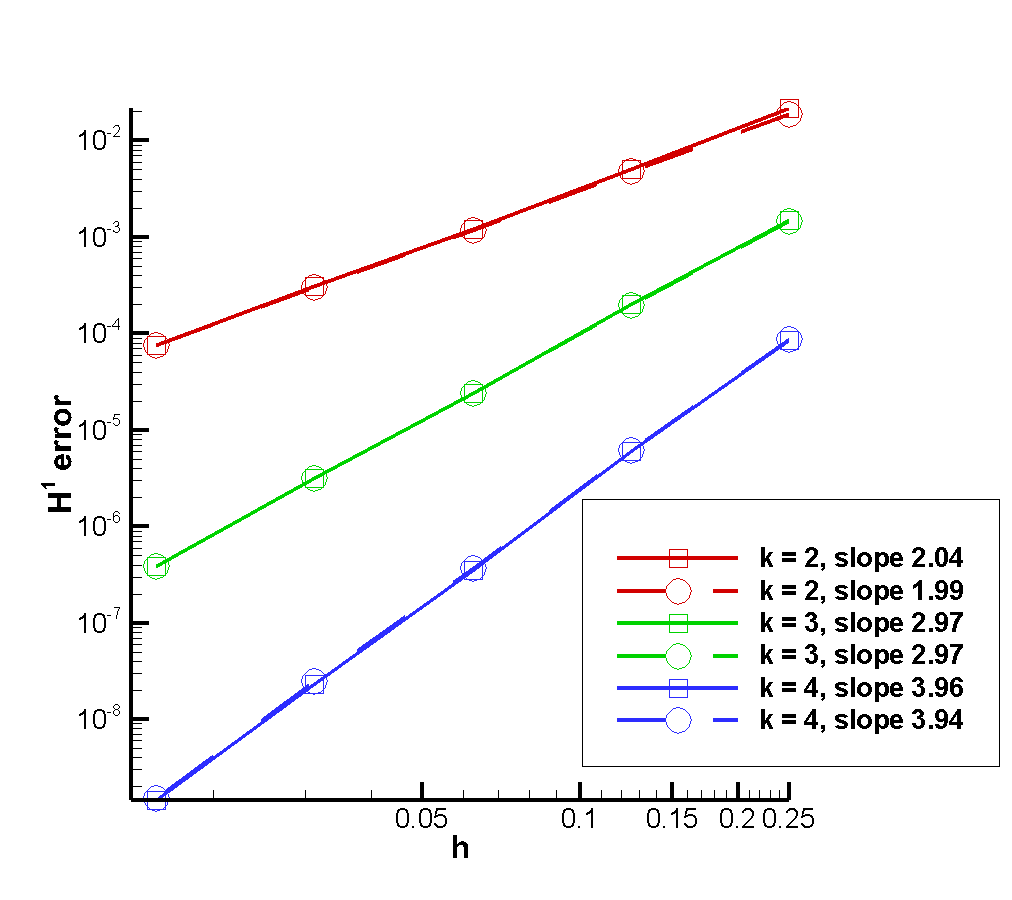
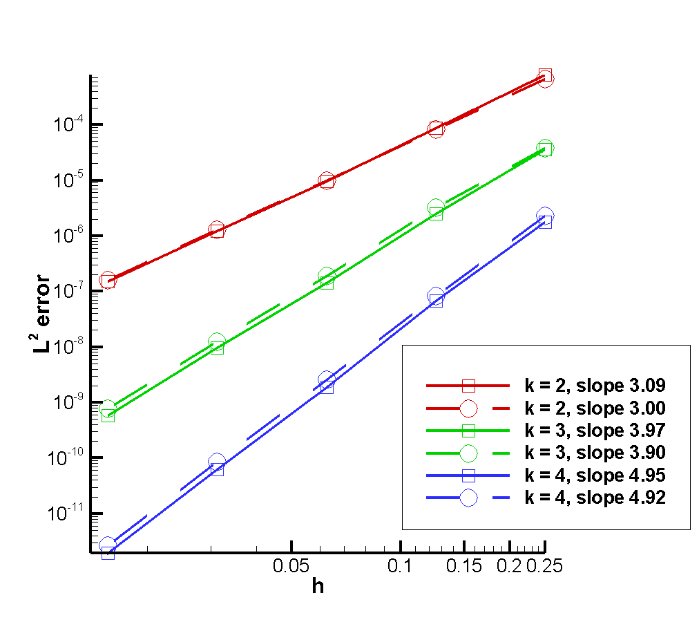
Figure 2: The test case with Poisson equation: the error in L2L^{2} norm and H1H^{1} semi-norm vs. mesh-size hh. The solid lines with squares represent the SIP method. The dashed lines with circles represent the scSIP method.

We have considered the Poisson equation, i.e. (1) with A=IA=I, on Ω=(0,1)2\Omega=(0,1)^{2} with homogeneous Dirichlet boundary conditions g=0g=0 and the exact solution u=sin⁡(π​x)​sin⁡(π​y)u=\sin(\pi x)\sin(\pi y). We have applied SIP method (11) and scSIP method (14)–(17) to this problem on the agglomerated meshes as described in the preamble of this Section. The results are presented in Fig. 2. In a slight deviation from the general notations, we set here the mesh-size as h=1/nh=1/n on the n×nn\times n mesh, and hE=hh_{E}=h on all the edges in (12). Three choices for the polynomial space degree kk were investigated, namely k=2,3,4k=2,3,4 and the penalty parameter γ\gamma in (12) was set to 2​k​(k+1)2k(k+1) (by a loose extrapolation to the polygonal meshes of the bound on the constant in the inverse inequality on a triangle in [23]). The numerical results confirm the theoretically expected order of convergence in both L2L^{2} norm and H1H^{1} semi-norm. They also demonstrate that the approximation produced by SIP and scSIP methods are very close to each other.

5.3 The second test case: non-constant coefficients AA
Refer to caption  Refer to caption

Figure 3: Test case with the non constant coefficient matrix AA: the error in L2L^{2} norm and H1H^{1} semi-norm vs. mesh-size hh. The solid lines with squares represent the SIP method. The dashed lines with circles represent the scSIP method.

We now consider problem (1) with a non-constant coefficient matrix

A=(1+xx​yx​y1+y)A=\left(\begin{array}[]{cc}1+x&xy\\ xy&1+y\end{array}\right)

set again on Ω=(0,1)2\Omega=(0,1)^{2}. The right-hand side ff and non-homogeneous Dirichlet boundary conditions gg are chosen so that the exact solution is given by u=ex​yu=e^{xy}. The results are presented in Fig. 3 using the same meshes and parameters hh, hEh_{E}, and γ\gamma as in the first test case. We arrive at the same conclusions about the convergence of SIP and scSIP methods as before.

Acknowledgements.
I am grateful to Simon Lemaire for interesting discussions about HHO and msHHO methods, which were the starting point of conceiving the present article.

References

  • (1) Adams, R.A.: Sobolev spaces. Academic Press [A subsidiary of Harcourt Brace Jovanovich, Publishers], New York-London (1975). Pure and Applied Mathematics, Vol. 65
  • (2) Antonietti, P.F., Cangiani, A., Collis, J., Dong, Z., Georgoulis, E.H., Giani, S., Houston, P.: Review of discontinuous galerkin finite element methods for partial differential equations on complicated domains. In [4] (2016)
  • (3) Arnold, D.N.: An interior penalty finite element method with discontinuous elements. SIAM J. Numer. Anal. 19(4), 742–760 (1982). URL https://doi.org/10.1137/0719052
  • (4) Barrenechea, G.R., Brezzi, F., Cangiani, A., Georgoulis, E.H. (eds.): Building bridges: connections and challenges in modern approaches to numerical partial differential equations, Lecture Notes in Computational Science and Engineering, vol. 114. Springer, [Cham] (2016). URL https://doi.org/10.1007/978-3-319-41640-3. Selected papers from the 101st LMS-EPSRC Symposium held at Durham University, Durham, July 8–16, 2014
  • (5) Brezzi, F., Marini, L.D.: Virtual element methods for plate bending problems. Comput. Methods Appl. Mech. Engrg. 253, 455–462 (2013). URL https://doi.org/10.1016/j.cma.2012.09.012
  • (6) Cangiani, A., Georgoulis, E.H., Houston, P.: h​php-version discontinuous Galerkin methods on polygonal and polyhedral meshes. Math. Models Methods Appl. Sci. 24(10), 2009–2041 (2014). DOI 10.1142/S0218202514500146. URL https://doi.org/10.1142/S0218202514500146
  • (7) Ciarlet, P.G.: Basic error estimates for elliptic problems. In: Handbook of numerical analysis, Vol. II, Handb. Numer. Anal., II, pp. 17–351. North-Holland, Amsterdam (1991)
  • (8) Cockburn, B.: Static condensation, hybridization, and the devising of the HDG methods. In: [4] (2016)
  • (9) Cockburn, B., Di Pietro, D.A., Ern, A.: Bridging the hybrid high-order and hybridizable discontinuous Galerkin methods. ESAIM Math. Model. Numer. Anal. 50(3), 635–650 (2016). URL https://doi.org/10.1051/m2an/2015051
  • (10) Cockburn, B., Gopalakrishnan, J., Lazarov, R.: Unified hybridization of discontinuous Galerkin, mixed, and continuous Galerkin methods for second order elliptic problems. SIAM J. Numer. Anal. 47(2), 1319–1365 (2009). URL https://doi.org/10.1137/070706616
  • (11) Di Pietro, D.A., Ern, A.: Mathematical aspects of discontinuous Galerkin methods, Mathématiques & Applications (Berlin) [Mathematics & Applications], vol. 69. Springer, Heidelberg (2012). URL https://doi.org/10.1007/978-3-642-22980-0
  • (12) Di Pietro, D.A., Ern, A.: A hybrid high-order locking-free method for linear elasticity on general meshes. Comput. Methods Appl. Mech. Engrg. 283, 1–21 (2015). URL https://doi.org/10.1016/j.cma.2014.09.009
  • (13) Di Pietro, D.A., Ern, A., Lemaire, S.: An arbitrary-order and compact-stencil discretization of diffusion on general meshes based on local reconstruction operators. Comput. Methods Appl. Math. 14(4), 461–472 (2014). URL https://doi.org/10.1515/cmam-2014-0018
  • (14) Di Pietro, D.A., Ern, A., Lemaire, S.: A review of hybrid high-order methods: formulations, computational aspects, comparison with other methods. In [4] (2016)
  • (15) Ern, A., Guermond, J.L.: Theory and practice of finite elements, Applied Mathematical Sciences, vol. 159. Springer-Verlag, New York (2004)
  • (16) Girault, V., Raviart, P.A.: Finite element methods for Navier-Stokes equations, Springer Series in Computational Mathematics, vol. 5. Springer-Verlag, Berlin (1986). DOI 10.1007/978-3-642-61623-5. URL https://doi.org/10.1007/978-3-642-61623-5. Theory and algorithms
  • (17) Guyan, R.J.: Reduction of stiffness and mass matrices. AIAA journal 3(2), 380 (1965)
  • (18) Hecht, F.: New development in freefem++. J. Numer. Math. 20(3-4), 251–265 (2012)
  • (19) Riviere, B.: Discontinuous Galerkin methods for solving elliptic and parabolic equations: theory and implementation. SIAM (2008)
  • (20) Beirão da Veiga, L., Brezzi, F., Marini, L.D.: Virtual elements for linear elasticity problems. SIAM J. Numer. Anal. 51(2), 794–812 (2013). URL https://doi.org/10.1137/120874746
  • (21) Beirão da Veiga, L., Brezzi, F., Marini, L.D., Russo, A.: Virtual element implementation for general elliptic equations. In [4] (2016)
  • (22) Wang, J., Ye, X.: A weak Galerkin finite element method for second-order elliptic problems. J. Comput. Appl. Math. 241, 103–115 (2013). URL https://doi.org/10.1016/j.cam.2012.10.003
  • (23) Warburton, T., Hesthaven, J.S.: On the constants in h​php-finite element trace inverse inequalities. Comput. Methods Appl. Mech. Engrg. 192(25), 2765–2773 (2003). DOI 10.1016/S0045-7825(03)00294-9. URL https://doi.org/10.1016/S0045-7825(03)00294-9
  • (24) Wheeler, M.F.: An elliptic collocation-finite element method with interior penalties. SIAM Journal on Numerical Analysis 15(1), 152–161 (1978)