Low Rank Matrix Approximation for Geometry Filtering
Abstract.
We propose a robust normal estimation method for both point clouds and meshes using a low rank matrix approximation algorithm. First, we compute a local isotropic structure for each point and find its similar, non-local structures that we organize into a matrix. We then show that a low rank matrix approximation algorithm can robustly estimate normals for both point clouds and meshes. Furthermore, we provide a new filtering method for point cloud data to smooth the position data to fit the estimated normals. We show applications of our method to point cloud filtering, point set upsampling, surface reconstruction, mesh denoising, and geometric texture removal. Our experiments show that our method outperforms current methods in both visual quality and accuracy.
Keywords:
Geometry filtering, Point cloud filtering, Mesh denoising, Point upsampling, Surface reconstruction, Geometric texture removal1. Introduction
Normal estimation for point cloud models or mesh shapes is important since it is often the first step in a geometry processing pipeline. This estimation is often followed by a filtering process to update the position data and remove noise [Sun et al., 2007]. A variety of computer graphics applications, such as point cloud filtering [Avron et al., 2010; Sun et al., 2015; Lu et al., 2017b], point set upsampling [Huang et al., 2013], surface reconstruction [Öztireli et al., 2009], mesh denoising [Sun et al., 2007; Zheng et al., 2011; Zhang et al., 2015b] and geometric texture removal [Wang et al., 2015] rely heavily on the quality of estimated normals and subsequent filtering of position data.
Current state of the art techniques in mesh denoising [Sun et al., 2007; Zheng et al., 2011; Zhang et al., 2015b] and geometric texture removal [Wang et al., 2015] can achieve impressive results. However, these methods are still limited in their ability to recover sharp edges in challenging regions. Normal estimation for point clouds has been an active area of research in recent years [Boulch and Marlet, 2012; Huang et al., 2013; Boulch and Marlet, 2016]. However, these methods perform suboptimally when estimating normals in noisy point clouds. Specifically, [Boulch and Marlet, 2012; Boulch and Marlet, 2016] are less robust in the presence of considerable noise. The bilateral filter can preserve geometric features but sometimes may fail due to the locality of its computations and lack of self-adaption of parameters.
Updating point positions using the estimated normals in point clouds has received sparse treatment so far [Avron et al., 2010; Sun et al., 2015]. However, those position update approaches using the or norms are complex to solve and hard to implement. Moreover, they restrict each point to only move along its normal orientation potentially leading to suboptimal results or slow convergence.
To address the issues shown above, we propose a new normal estimation method for both meshes and point clouds and a new position update algorithm for point clouds. Our method benefits various geometry processing applications, directly or indirectly, such as point cloud filtering, point set upsampling, surface reconstruction, mesh denoising, and geometric texture removal (Figure 1). Given a point cloud or mesh as input, our method first estimates point or face normals, then updates the positions of points or vertices using the estimated normals. We observe that: (1) non-local methods could be more accurate than local techniques; (2) there usually exist similar structures of each local isotropic structure (Section 3.1) in geometry shapes; (3) the matrix constructed by similar structures should be low-rank. Motivated by these observations, we propose a novel normal estimation technique which consists of two sub-steps: (i) non-local similar structures location and (ii) weighted nuclear norm minimization. We adopt the former to find similar structures of each local isotropic structure. We employ the latter [Gu et al., 2014] to handle the problem of recovering low-rank matrices. We also present a fast and effective point update algorithm for point clouds to filter the point positions to better match the estimated normals.
The main contributions of this paper are:
- •
a novel normal estimation technique for both point cloud shapes and mesh models;
- •
a new position update algorithm for point cloud data;
- •
analysis of the convergence of the proposed normal estimation technique and point update algorithm, experimentally or theoretically.
Extensive experiments and comparisons show that our method outperforms current methods in terms of visual quality and accuracy.
2. Related Work
In this section, we only review the research works that are most related to this work. We first review the previous research on normal estimation. Then we review some previous works which employed the nuclear norm minimization or its weighted version.
2.1. Normal Estimation
Normal estimation for geometric shapes can be classified into two types: (1) normal estimation for point clouds, and (2) normal estimation for mesh shapes.
Normal estimation for point clouds. Hoppe et al. [Hoppe et al., 1992] estimated normals by computing the tangent plane at each data point using principal component analysis (PCA) of the local neighborhood. Later, a variety of variants of PCA have been proposed [Alexa et al., 2001; Pauly et al., 2002; Mitra and Nguyen, 2003; Lange and Polthier, 2005; Huang et al., 2009] to estimate normals. Nevertheless, the normals estimated by these techniques tend to smear sharp features. Researchers also estimate normals using Voronoi cells or Voronoi-PCA [Dey and Goswami, 2004; Alliez et al., 2007]. Minimizing the or norm can preserve sharp features as these norms can be used to measure sparsity in the derivative of the normal field [Avron et al., 2010; Sun et al., 2015]. Yet, the solutions are complex and computationally expensive. Li et al. [Li et al., 2010] estimated normals by using robust statistics to detect the best local tangent plane for each point. Another set of techniques attempted to better estimate normals near edges and corners by point clustering in a neighborhood [Zhang et al., 2013; Liu et al., 2015]. Later they presented a pair consistency voting scheme which outputs multiple normals per feature point [Zhang et al., 2018]. Boulch and Marlet [Boulch and Marlet, 2012] use a robust randomized Hough transform to estimate point normals. Convolutional neural networks have recently been applied to estimate normals in point clouds [Boulch and Marlet, 2016]. Such estimation methods are usually less robust for point clouds with considerable amount of noise. Bilateral smoothing of PCA normals [Öztireli et al., 2009; Huang et al., 2013] is simple and effective, but it suffers from inaccuracy due to the locality of its computations and may blur edges with small dihedral angles.
Normal estimation for mesh shapes. Most methods focus on the estimation of face normals in mesh shapes. One simple, direct way is to compute the face normals by the cross product of two edges in a triangle face. However, such normals can deviate from the true normals significantly even in the presence of small position noise. There exist a considerable amount of research work to smooth these face normals. One approach uses the bilateral filter [Lee and Wang, 2005; Wang, 2006; Zheng et al., 2011], inspired by the founding works [Jones et al., 2003; Fleishman et al., 2003]. Mean, median and alpha-trimming methods [Yagou et al., 2002; Yagou et al., 2003; Shen and Barner, 2004] are also used to estimate face normals. Sun et al. [Sun et al., 2007; Sun et al., 2008] present two different methods to filter face normals. Recently, researchers have presented filtering methods [Solomon et al., 2014; Zhang et al., 2015b; Zhang et al., 2015a; Lu et al., 2017a; Yadav et al., 2017] based on mean shift, total variation, guided normals, median, and normal voting tensor. Wang et al. [Wang et al., 2016] estimated face normals via cascaded normal regression.
2.2. Nonlocal Methods for Point Clouds and Nuclear Norm Minimization
Previous researchers proposed non-local methods for point clouds. For example, Zheng et al. [Zheng et al., 2010] applied non-local filtering to 3D buildings that exhibit large scale repetitions and self-similarities. Digne presented a non-local denoising framework to unorganized point clouds by building an intrinsic descriptor [Digne, 2012], and recently proposed a shape analysis approach with colleagues based on the non-local analysis of local shape variations [Digne et al., 2018].
The nuclear norm of a matrix is defined as the sum of the absolute values of its singular values (see Eq. (3)). It has been proved that most low-rank matrices can be recovered by minimizing their nuclear norm [Candès and Recht, 2009]. Cai et al. [Cai et al., 2010] provided a simple solution to the low-rank matrix approximation problem by minimizing the nuclear norm. The nuclear norm minimization has been broadly employed to matrix completion [Candès and Recht, 2009; Cai et al., 2010], robust principle component analysis [Wright et al., 2009], low-rank representation for subspace clustering [Liu et al., 2010] and low-rank textures [Zhang et al., 2012]. Gu et al. [Gu et al., 2014; Gu et al., 2017] presented a weighted version of the nuclear norm minimization, which has been adopted to image processing applications such as image denoising, background subtraction and image inpainting.
3. Normal Estimation
In this section, we take point clouds, consisting of positions as well as normals, as input and further extend to meshes later. First of all, we present an algorithm to locate and construct non-local similar structures for each local isotropic structure of a point (Section 3.1). We then describe how to estimate normals via weighted nuclear norm minimization on non-local similar structures (Section 3.2).
3.1. Non-local Similar Structures
Local structure. We define each point has a local structure which consists of nearest neighbors. Locating structures similar to a specific local structure is difficult due to the irregularity of points.
Tensor voting. We assume each local structure embeds a representative orientation. To do so, we first define the tensor at a point as
| (1) |
where ( vector) is one of the nearest neighbors of , which we denote as , and ( vector) is the normal of . and are the weights induced by spatial distances and intersection angles () of two neighboring normals, which are given by [Huang et al., 2013; Zheng et al., 2011]: , . and are the scaling parameters, which are empirically set to two times the maximal distance between any two points in the nearest neighbors within the local structure and , respectively.
For each local structure , we can derive the accumulated tensor by aggregating all the induced tensor votes . This final tensor encodes the local structure, which provides a reliable, representative orientation that will be later used to compute the local isotropic structure and locate similar structures.
| (2) |
Let be the eigenvalues of with the corresponding eigenvectors , and . In tensor voting [Wu et al., 2012], indicates surface saliency with a normal direction ; indicates curve saliency with a tangent orientation ; denotes junction saliency. Therefore, we take as the representative orientation for the local structure of point .


Local isotropic structure. We assume that each local structure has a subset of points that are on the same isotropic surface with the representative orientation. We call this subset of points the local isotropic structure. Now we describe how to obtain a local isotropic structure from a local structure and locate similar local isotropic structures for . We present a simple and effective way to achieve this: comparing the intersection angles of two normals. Specifically, to obtain , we
- •
compute the intersection angles between each point normal and the representative orientation within a local structure ;
- •
add the current point to if the corresponding intersection angle is less than or equal to a threshold, .
For simplicity, we will refer to similar local isotropic structures as similar structures. Given an isotropic structure , we identify its non-local similar structures by comparing the angles between the representative orientation of each structure. If the angle is less than or equal to (we use the same threshold for simplicity), we define the two isotropic structures to be similar. The underlying rationale of our similarity search is: the point normals in a local isotropic structure are bounded by the representative orientation, indicating these points are on the same isotropic surface; the similar structures search is also bounded by the representative orientations, implying the similar structures are on the similar isotropic surfaces. These similar structures will often overlap on the same isotropic surface as shown in Figure 2. In the figure, we show the local structure (a), the local isotropic structure (b), and the similar structures (c).
Remark 1. We do not consider other types of similarity such as rotation-invariant similarity which is often sensitive to noise. Moreover, the rotation quantities have to be estimated in the presence of noise. It could also introduce significant computational overhead to both similarity search and the following SVD operation. Even though our method does not have such a property, we observe it works very well for a wide range of models (see Section 5).
3.2. Weighted Nuclear Norm Minimization
For each non-local similar structure for the isotropic structure associated with the point , we append the point normals of as rows to a matrix . Note that the dimensions of this matrix are . This matrix already has a maximal rank of 3 and is a low rank matrix. To make the low rank matrix approximation meaningful, we reshape the matrix to be close to a square matrix.
We do so by finding dimensions and of a new matrix where and we minimize . Given that the structure in is isotropic, removing one or more points does not affect this structure significantly. Therefore, we find and iteratively by measuring if . If so, we remove a point normal from and solve for , again. We repeat such a process until ( is not constrained to be a multiple of three). Then we simply copy the column entries in to filling each column of before continuing to the next column. The resulting matrix should be low rank since all point normals come from similar isotropic structures.
We then cast the normal estimation problem as a low-rank matrix approximation problem. We attempt to recover a low-rank matrix from using nuclear norm minimization. We first present some fundamental knowledge about nuclear norm minimization and then show how we estimate normals with weighted nuclear norm minimization.


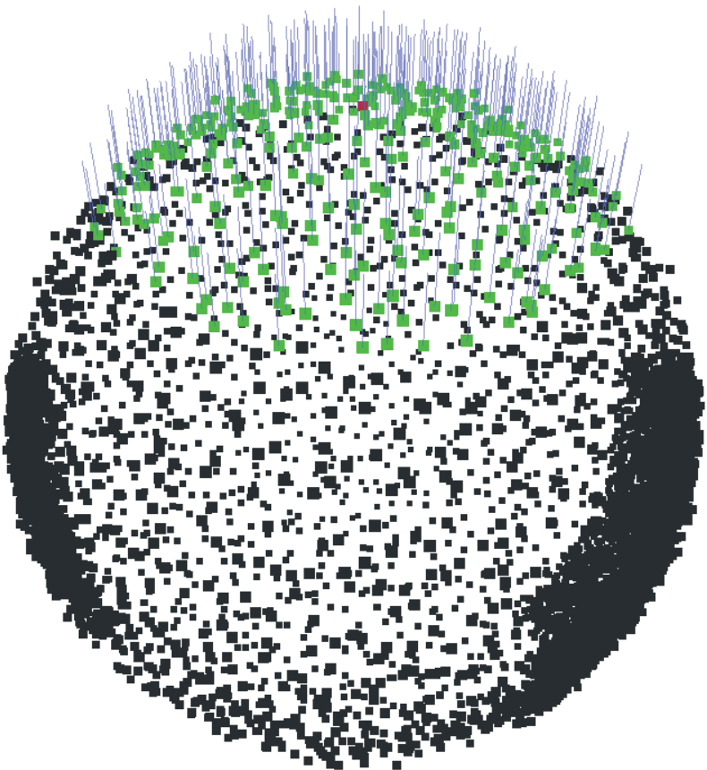


Nuclear norm. The nuclear norm of a matrix is defined as the sum of the absolute values of its singular values, shown in Eq. (3).
| (3) |
where is the -th singular value of matrix . indicates the nuclear norm of .
Nuclear norm minimization. Nuclear norm minimization is frequently used to approximate the known matrix, , by a low-rank matrix, , while minimizing the nuclear norm of . Cai et al. [Cai et al., 2010] demonstrated that the low-rank matrix can be easily solved by adding a Frobenius-norm data term.
| (4) |
where is the weighting parameter. The minimizing matrix is then
| (5) |
where denotes the SVD of and is the -th diagonal element in . is the soft-thresholding function on and the parameter , i.e., .
Nuclear norm minimization treats and shrinks each singular value equally. However, in general, larger singular values should be shrunk less to better approximate the known matrix and preserve the major components. The weighted nuclear norm minimization solves this issue [Gu et al., 2014].
Weighted nuclear norm minimization. The weighted nuclear norm of a matrix is
| (6) |
where is the non-negative weight imposed on the -th singular value and . We can then write the low-rank matrix approximation problem as
| (7) |
Suppose the singular values are sorted in a non-ascending order, the corresponding weights should be in a non-descending order. Hence, we define the weight function as a Gaussian function.
| (8) |
denotes the regularized coefficient which defaults to . is the first singular value after sorting in a non-increasing order. We did not use the original weight definition in [Gu et al., 2014] since it needs noise variance which should be unknown in normal estimation. Also, we found their weight determination is not suitable for normal-constructed matrices. Then we solve Eq. (7) by the generalized soft thresholding operation on the singular values with weights [Gu et al., 2014].
| (9) |
where . Here changes to the generalized soft-thresholding function by assigning weights to singular values, and Eq. (9) becomes the weighted version of Eq. (5).
Remark 2: matrix ordering. We investigated the ordering of the constructed matrix. We found that the ordering of points significantly influences the minimization result (Figure 3). We suspect this is due to the neighboring information and three coordinates of each normal in different ordering matrices, which is more complicated than the regular single-channel grayscale images.
Remark 3: and averaging. We tested the effects of averaging and . We found that is related to the number of ranks after the generalized soft-thresholding. A smaller leads to more ranks retained, which also indicates more noise is left behind. For instance, the numbers of ranks for the sphere example (Fig. 4) with , and are 147, 85 and 1, respectively. We also observed that the number of ranks is related to capturing changes in the surface: a greater captures less surface changes (e.g., Figure 4(b,e)). We found no relations between averaging and the most low-rank method (i.e., with the largest rank retained). The most low-rank method may also recover normals of a matrix with different directions (Figure 4(a,b)). Figure 4 (d-f) show that our default is more robust than both averaging and the most low-rank method.


3.3. Algorithm
Each point may have multiple normals in the recovered matrices , as the similar structures often overlap. We compute the final normal of each point by simply averaging the corresponding normals in after calling Algorithm 1. To achieve quality normal estimations, we iterate non-local similar structures clustering (Section 3.1) and the weighted nuclear norm minimization in Algorithm 1. Notice that our normal estimation algorithm is feature-aware, because each matrix consists only of similar local isotropic structures. Our normal estimation technique is more accurate and robust than the bilateral filter [Huang et al., 2013] when handling irregularly sampled data (Figure 5).
Extension to mesh models. Our algorithm can be easily extended to handle mesh models. One natural way is to take the vertices/normals of a mesh as points/normals in a point cloud. However, to achieve desired results, face normals are frequently used to update vertex positions [Sun et al., 2007; Zheng et al., 2011; Zhang et al., 2015b]. Hence, we use the centers of faces and the corresponding normals as points. Moreover, we use the mesh topology to compute neighbors in Section 3.1.


Convergence. As with the reported results of previous techniques [Zheng et al., 2011; Sun et al., 2007; Zhang et al., 2015b], we also cannot guarantee the convergence of our normal estimation method. Figure 7(a) shows a comparison between the bilateral filter [Huang et al., 2013] and our method as the iteration count increases. The figure indicates that our method is more accurate than the bilateral filter [Huang et al., 2013].
4. Position Update
Besides normal estimation, we also present algorithms to update point or vertex positions to match the estimated normals, which is typically necessary before applying other geometry processing algorithms.
Vertex update for mesh models. We use the algorithm [Sun et al., 2007] to update vertices of mesh models, which minimizes the square of the dot product between the normal and the three edges of each face.
Point update for point clouds. Compared to the vertex update for mesh models, updating point cloud positions is more difficult due to the absence of topological information. Furthermore, the local neighborhood information may vary during this position update. We propose a modification of the edge recovery algorithm in [Sun et al., 2015] to update points in a feature-aware way and minimize
| (10) |
and are unknown, and and are computed by our normal estimation algorithm. Eq. (10) encodes the sum of distances to the tangent planes defined by the neighboring points and the corresponding normals , as well as the sum of distances to the tangent planes defined by and . We use the gradient descent method to solve Eq. (10), by assuming the point and its neighboring points in the previous iteration are known. Here we use ball neighbors instead of k nearest neighbors to ensure the convergence of our point update. Therefore, the new position of can be computed by
| (11) |
where is the new position. is the step size, which is set to to ensure the convergence (see Appendix).
Remark 4. While the neighboring information for point updating should be recomputed in each iteration, doing so can lead to artifacts. As illustrated in Figure 8(a), our point update method enhances edges by automatically driving neighboring points to edges but also leads to obvious gaps near edges. As a result, the upsampling application could fail when the number of points is low (Figure 8(b)). To alleviate this issue, we simply keep the neighboring information unchanged in all iterations, which has the side-effect of reducing the computation in each iteration. Figure 8 shows a comparison. Though we cannot guarantee that our point update method preserves the volume of the shape, we found insignificant volume changes in our experiments. We show the proof of convergence of our point update algorithm in the Appendix.
5. Applications and Experimental Results
In this section, we demonstrate some geometry processing applications that benefit from our approach directly or indirectly including mesh denoising, point cloud filtering, point cloud upsampling, surface reconstruction, and geometric texture removal. Moreover, we also compared state of the art methods with our approach in each application. The source code (program) of the compared methods are available on the Internet or granted to us by the original authors.
Parameter setting. The main parameters of our normal estimation method are the local neighborhood size , the angle threshold , the non-local searching range , and the maximum iterations for normal estimation . For the position update procedure, our parameters are the local neighborhood size or 1-ring neighbors (mesh models) and the number of iterations for the position update .
To more accurately find similar local isotropic structures, we set one initial value and one lower bound to , namely and . We reduce the start value towards at a rate of in the -th iteration. We show the tests of our parameters in Figure 7 and 13. In general, normal errors are decreased with the growing number of normal estimation iterations, but excessive iterations would cause greater normal errors (Figure 7(a)). The estimated normals of models with sharp features are more accurate with the increasing local neighborhood or non-local search range (Figure 7(b)). However, we need to compromise between accuracy and computation. Fixed are likely to inaccurately locate similar local isotropic structures and further generate erroneous normal estimations (Figure 13(a-b)). Larger start values of smear geometric features (Figure 13(c)).
Based on our parameter tests and observations, for point clouds we empirically set: , , , and for models with sharp features, but set and for models with low dihedral angle features. For mesh models, we replace the local neighborhood with the 2-ring of neighboring faces. We use 4 to 10 iterations for normal estimation and 5 to 30 for the position update.
For fair comparisons, we set the same local neighborhood to other methods. The remaining parameters of other methods are tuned to achieve the best visual results. Regarding [Boulch and Marlet, 2012; Boulch and Marlet, 2016], the two methods have multiple solutions and the best results are selected for comparisons. For the position update, we set the same parameters for the compared normal estimation methods for each model.


Accuracy. Since we used the pre-filter [Lu et al., 2016] for meshes with large noise, there exist few flipped normals in the results so that different methods have limited difference in normal accuracy. However, the visual differences are easy to observe. Therefore, we compared the accuracies of normals and positions over point cloud shapes. Note that state of the art methods compute normals on edges differently: the normals on edges are either sideling (e.g., [Hoppe et al., 1992; Boulch and Marlet, 2016]) or perpendicular to one of the intersected tangent planes (e.g., [Huang et al., 2013] and our method). The latter is more suitable for feature-aware position update. For fair comparisons, we have two ground truth models for each point cloud: the original ground truth for [Hoppe et al., 1992; Boulch and Marlet, 2016] and the other ground truth for [Huang et al., 2013] and our method. The latter ground truth is generated by adapting normals on edges to be perpendicular to one of the intersected tangent planes. The ground truth model, which has the smaller mean square angular error (MSAE) [Lu et al., 2016] among the two kinds of ground truth models, is selected as the ground truth for [Boulch and Marlet, 2012]. Figure 14 shows the normal errors of different levels of noise on the cube and dodecahedron models. We also compared our method with state of the art techniques in Table 1. The ground truth for the Dod_vir model (Table 1) for [Hoppe et al., 1992; Boulch and Marlet, 2016] is achieved by averaging the neighboring face normals in the noise-free model. The other kind of ground truth for [Huang et al., 2013] and our method is produced by further adapting normals on edges to one of the intersected tangent planes. We compute ground truth for Figure 12 and 14 in a similar way. The normal error results demonstrate that our approach outperforms state of the art methods. We analyzed that this is probably due to more exhibited useful information of non-local similar structures than local techniques.
| Methods |
|
|
|
|
| |||||||||
|---|---|---|---|---|---|---|---|---|---|---|---|---|---|---|
| Dod_vir | 0.0150 | 0.0465 | 0.0054 | 0.0553 | 0.0023 | |||||||||
| Fig. 12 | 0.0118 | 0.1274 | 0.0060 | 0.1208 | 0.0036 |
In addition, we compared the position errors of different techniques, see Figure 17 and 18. The position error is measured using the average distance between points of the ground truth and their closest points of the reconstructed point set [Lu et al., 2017b]. For visualization purpose, we rendered the colors of position errors on the upsampling results. The root mean square error (RMSE) of both the upsampling and reconstruction results show that our approach is more accurate than state of the art methods.


5.1. Point Cloud Filtering
We compare our normal estimation method with several state of the art normal estimation techniques. We then perform the same number of iterations of our position update algorithm with the estimated normals of all methods.
Figure 6 and 9 show two point cloud models corrupted with heavy, synthetic noise. The results demonstrate that our method performs better than state of the art approaches in terms of feature preservation and non-feature smoothness. Figure 10, 11, 12, and 15 show the methods applied to a variety of real scanned point cloud models. Our approach outperforms other methods in terms of the quality of the estimated normals. We demonstrate our technique on point clouds with more complicated features. Figure 20 shows that our method produces slightly lower normal errors than [Huang et al., 2013]. Figure 20 (f) and (g) show our method with different parameters, which leads to a less/more sharpened version of the input. We also show some results using [Huang et al., 2009; Preiner et al., 2014], which do not preserve sharp features (Figure 19).
5.2. Point Cloud Upsampling
As described in Section 5.1, the point cloud filtering also consists of a two-step procedure: normal estimation and point update. However, unlike mesh shapes, point cloud models often need to be resampled to enhance point density after filtering operations have been applied.
We apply the edge-aware point set resampling technique [Huang et al., 2013] to all the results after point cloud filtering and contrast the different upsampling results. For fair comparisons, we upsample the filtered point clouds of each model to reach a similar number of points. Figure 6 to 15 display various upsampling results on state of the art normal estimation methods and different point cloud models. The figures show that the upsampling results on our filtered point clouds are substantially better than those filtered by other methods in preserving geometric features. Bilateral normal smoothing [Huang et al., 2013] usually produces good results, but this method sometimes blur edges with low dihedral angles.
5.3. Surface Reconstruction
One common application for point cloud models is to reconstruct surfaces from the upsampled point clouds in Section 5.2 before use in other applications. Here, we select the edge-aware surface reconstruction technique–RIMLS [Öztireli et al., 2009]. For fair comparisons, we use the same parameters for all the upsampled point clouds of each model.
5.4. Mesh Denoising
Many state of the art mesh denoising methods involve a two-step procedure which first estimates normals and then updates vertex positions. We selected several of these methods [Sun et al., 2007; Zheng et al., 2011; Zhang et al., 2015b] for comparisons in Figure 16. Note that [Zheng et al., 2011] provides both a local and global solution, and we provide comparisons for both.
When the noise level is high, many of these methods produce flipped face normals. For the Bunny model (Figure 16), which involves frequent flipped triangles, we utilize the technique in [Lu et al., 2016] to estimate a starting mesh from the original noisy mesh input for all methods. The comparison results show that our method outperforms state of the art mesh denoising methods in terms of feature preservation.
5.5. Geometric Texture Removal
We also successfully applied our method to geometric de-texturing where we remove high frequency features of different scales. Figure 21 shows comparisons of different methods that demonstrate that our method outperforms other approaches. Note that [Wang et al., 2015] is specifically designed for geometric texture removal. However, that method cannot preserve sharp edges well. Figure 22 shows the results of removing different scales of geometric features on a mesh. We produced Figure 22 (d) by applying the pre-filtering technique [Lu et al., 2016] in advance, since the vertex update algorithm [Zheng et al., 2011] could generate frequent flipped triangles when dealing with such large and steep geometric features. As an alternative, our normal estimation method can be combined with the vertex update in [Wang et al., 2015] to handle such challenging mesh models. Figure 23 shows the geometric texture removal on two different point clouds, which are particularly challenging due to a lack of topology.


| Methods |
|
|
|
|
|
| ||||||||||||
|---|---|---|---|---|---|---|---|---|---|---|---|---|---|---|---|---|---|---|
|
0.57 | 141.5 | 0.48 | 8 | 95.6 | 65.1 | ||||||||||||
|
18.7 | 2204 | 17.2 | 115 | 3147 | 2458 | ||||||||||||
|
10.8 | 3769 | 12.5 | 141 | 3874 | 2856 |
5.6. Timings
Table 2 summarizes the timings of different normal estimation methods on several point clouds. While our method produces high quality output, the algorithm takes a long time to run due to the svd operation for each normal estimation. Therefore, our method is more suitable for offline geometry processing. However, it is possible to accelerate our method using specific svd decomposition algorithms, such as the randomized svd (RSVD) decomposition algorithm [Halko et al., 2011] as shown in Table 2. In addition, many parts of the algorithm could benefit from parallelization.
6. Conclusion
In this paper, we have presented an approach consisting of two steps: normal estimation and position update. Our method can handle both mesh shapes and point cloud models. We also show various geometry processing applications that benefit from our approach directly or indirectly. The extensive experiments demonstrate that our method performs substantially better than state of the art techniques, in terms of both visual quality and accuracy.
While our method works well, speed is an issue if online processing speeds are required. In addition, though we mitigate issues associated with the point distribution in the position update procedure, the point distribution could still be improved. One way to do so is to re-distribute points after our position update through a “repulsion force” from each point to its neighbors. We could potentially accomplish this effect by adding this repulsion force directly to Eq. (10).
References
- Alexa et al. [2001] Marc Alexa, Johannes Behr, Daniel Cohen-Or, Shachar Fleishman, David Levin, and Claudio T. Silva. 2001. Point Set Surfaces. In Proceedings of the Conference on Visualization ’01 (VIS ’01). IEEE Computer Society, Washington, DC, USA, 21–28. http://dl.acm.org/citation.cfm?id=601671.601673
- Alliez et al. [2007] P. Alliez, D. Cohen-Steiner, Y. Tong, and M. Desbrun. 2007. Voronoi-based Variational Reconstruction of Unoriented Point Sets. In Proceedings of the Fifth Eurographics Symposium on Geometry Processing (SGP ’07). Eurographics Association, Aire-la-Ville, Switzerland, Switzerland, 39–48. http://dl.acm.org/citation.cfm?id=1281991.1281997
- Avron et al. [2010] Haim Avron, Andrei Sharf, Chen Greif, and Daniel Cohen-Or. 2010. L1-Sparse Reconstruction of Sharp Point Set Surfaces. ACM Trans. Graph. 29, 5, Article 135 (Nov. 2010), 12 pages. https://doi.org/10.1145/1857907.1857911
- Boulch and Marlet [2012] Alexandre Boulch and Renaud Marlet. 2012. Fast and Robust Normal Estimation for Point Clouds with Sharp Features. Comput. Graph. Forum 31, 5 (Aug. 2012), 1765–1774. https://doi.org/10.1111/j.1467-8659.2012.03181.x
- Boulch and Marlet [2016] Alexandre Boulch and Renaud Marlet. 2016. Deep Learning for Robust Normal Estimation in Unstructured Point Clouds. Computer Graphics Forum 35, 5 (2016), 281–290. https://doi.org/10.1111/cgf.12983
- Cai et al. [2010] Jian-Feng Cai, Emmanuel J. Candès, and Zuowei Shen. 2010. A Singular Value Thresholding Algorithm for Matrix Completion. SIAM J. on Optimization 20, 4 (March 2010), 1956–1982. https://doi.org/10.1137/080738970
- Candès and Recht [2009] Emmanuel J. Candès and Benjamin Recht. 2009. Exact Matrix Completion via Convex Optimization. Foundations of Computational Mathematics 9, 6 (03 Apr 2009), 717. https://doi.org/10.1007/s10208-009-9045-5
- Dey and Goswami [2004] Tamal K. Dey and Samrat Goswami. 2004. Provable Surface Reconstruction from Noisy Samples. In Proceedings of the Twentieth Annual Symposium on Computational Geometry (SCG ’04). ACM, New York, NY, USA, 330–339. https://doi.org/10.1145/997817.997867
- Digne [2012] J. Digne. 2012. Similarity based filtering of point clouds. In 2012 IEEE Computer Society Conference on Computer Vision and Pattern Recognition Workshops. 73–79. https://doi.org/10.1109/CVPRW.2012.6238917
- Digne et al. [2018] J. Digne, S. Valette, and R. Chaine. 2018. Sparse Geometric Representation Through Local Shape Probing. IEEE Transactions on Visualization and Computer Graphics 24, 7 (July 2018), 2238–2250. https://doi.org/10.1109/TVCG.2017.2719024
- Fleishman et al. [2003] Shachar Fleishman, Iddo Drori, and Daniel Cohen-Or. 2003. Bilateral Mesh Denoising. ACM Trans. Graph. 22, 3 (July 2003), 950–953. https://doi.org/10.1145/882262.882368
- Gu et al. [2017] Shuhang Gu, Qi Xie, Deyu Meng, Wangmeng Zuo, Xiangchu Feng, and Lei Zhang. 2017. Weighted Nuclear Norm Minimization and Its Applications to Low Level Vision. International Journal of Computer Vision 121, 2 (01 Jan 2017), 183–208. https://doi.org/10.1007/s11263-016-0930-5
- Gu et al. [2014] Shuhang Gu, Lei Zhang, Wangmeng Zuo, and Xiangchu Feng. 2014. Weighted Nuclear Norm Minimization with Application to Image Denoising. In Proceedings of the 2014 IEEE Conference on Computer Vision and Pattern Recognition (CVPR ’14). IEEE Computer Society, Washington, DC, USA, 2862–2869. https://doi.org/10.1109/CVPR.2014.366
- Halko et al. [2011] N. Halko, P. G. Martinsson, and J. A. Tropp. 2011. Finding Structure with Randomness: Probabilistic Algorithms for Constructing Approximate Matrix Decompositions. SIAM Rev. 53, 2 (2011), 217–288. https://doi.org/10.1137/090771806 arXiv:https://doi.org/10.1137/090771806
- He and Schaefer [2013] Lei He and Scott Schaefer. 2013. Mesh Denoising via L0 Minimization. ACM Trans. Graph. 32, 4, Article 64 (July 2013), 8 pages. https://doi.org/10.1145/2461912.2461965
- Hoppe et al. [1992] Hugues Hoppe, Tony DeRose, Tom Duchamp, John McDonald, and Werner Stuetzle. 1992. Surface Reconstruction from Unorganized Points. SIGGRAPH Comput. Graph. 26, 2 (July 1992), 71–78. https://doi.org/10.1145/142920.134011
- Huang et al. [2009] Hui Huang, Dan Li, Hao Zhang, Uri Ascher, and Daniel Cohen-Or. 2009. Consolidation of Unorganized Point Clouds for Surface Reconstruction. ACM Trans. Graph. 28, 5, Article 176 (Dec. 2009), 7 pages. https://doi.org/10.1145/1618452.1618522
- Huang et al. [2013] Hui Huang, Shihao Wu, Minglun Gong, Daniel Cohen-Or, Uri Ascher, and Hao (Richard) Zhang. 2013. Edge-aware Point Set Resampling. ACM Trans. Graph. 32, 1, Article 9 (Feb. 2013), 12 pages. https://doi.org/10.1145/2421636.2421645
- Jones et al. [2003] Thouis R. Jones, Frédo Durand, and Mathieu Desbrun. 2003. Non-iterative, Feature-preserving Mesh Smoothing. ACM Trans. Graph. 22, 3 (July 2003), 943–949. https://doi.org/10.1145/882262.882367
- Lange and Polthier [2005] Carsten Lange and Konrad Polthier. 2005. Anisotropic smoothing of point sets. Computer Aided Geometric Design 22, 7 (2005), 680 – 692. https://doi.org/10.1016/j.cagd.2005.06.010 Geometric Modelling and Differential Geometry.
- Lee and Wang [2005] Kai-Wah Lee and Wen-Ping Wang. 2005. Feature-preserving mesh denoising via bilateral normal filtering. In Proc. of Int’l Conf. on Computer Aided Design and Computer Graphics 2005.
- Li et al. [2010] Bao Li, Ruwen Schnabel, Reinhard Klein, Zhiquan Cheng, Gang Dang, and Shiyao Jin. 2010. Robust normal estimation for point clouds with sharp features. Computers & Graphics 34, 2 (2010), 94 – 106. https://doi.org/10.1016/j.cag.2010.01.004
- Liu et al. [2010] Guangcan Liu, Zhouchen Lin, and Yong Yu. 2010. Robust Subspace Segmentation by Low-rank Representation. In Proceedings of the 27th International Conference on International Conference on Machine Learning (ICML’10). Omnipress, USA, 663–670. http://dl.acm.org/citation.cfm?id=3104322.3104407
- Liu et al. [2015] Xiuping Liu, Jie Zhang, Junjie Cao, Bo Li, and Ligang Liu. 2015. Quality point cloud normal estimation by guided least squares representation. Computers & Graphics 51, Supplement C (2015), 106 – 116. https://doi.org/10.1016/j.cag.2015.05.024 International Conference Shape Modeling International.
- Lu et al. [2017a] Xuequan Lu, Wenzhi Chen, and Scott Schaefer. 2017a. Robust mesh denoising via vertex pre-filtering and L1-median normal filtering. Computer Aided Geometric Design 54, Supplement C (2017), 49 – 60. https://doi.org/10.1016/j.cagd.2017.02.011
- Lu et al. [2016] Xuequan Lu, Zhigang Deng, and Wenzhi Chen. 2016. A Robust Scheme for Feature-Preserving Mesh Denoising. IEEE Trans. Vis. Comput. Graph. 22, 3 (2016), 1181–1194.
- Lu et al. [2017b] X. Lu, S. Wu, H. Chen, S. K. Yeung, W. Chen, and M. Zwicker. 2017b. GPF: GMM-inspired Feature-preserving Point Set Filtering. IEEE Transactions on Visualization and Computer Graphics PP, 99 (2017), 1–1. https://doi.org/10.1109/TVCG.2017.2725948
- Mitra and Nguyen [2003] Niloy J. Mitra and An Nguyen. 2003. Estimating Surface Normals in Noisy Point Cloud Data. In Proceedings of the Nineteenth Annual Symposium on Computational Geometry (SCG ’03). ACM, New York, NY, USA, 322–328. https://doi.org/10.1145/777792.777840
- Öztireli et al. [2009] A. C. Öztireli, G. Guennebaud, and M. Gross. 2009. Feature Preserving Point Set Surfaces based on Non-Linear Kernel Regression. Computer Graphics Forum 28, 2 (2009), 493–501. https://doi.org/10.1111/j.1467-8659.2009.01388.x
- Pauly et al. [2002] Mark Pauly, Markus Gross, and Leif P. Kobbelt. 2002. Efficient Simplification of Point-sampled Surfaces. In Proceedings of the Conference on Visualization ’02 (VIS ’02). IEEE Computer Society, Washington, DC, USA, 163–170. http://dl.acm.org/citation.cfm?id=602099.602123
- Preiner et al. [2014] Reinhold Preiner, Oliver Mattausch, Murat Arikan, Renato Pajarola, and Michael Wimmer. 2014. Continuous Projection for Fast L1 Reconstruction. ACM Trans. Graph. 33, 4, Article 47 (July 2014), 13 pages. https://doi.org/10.1145/2601097.2601172
- Shen and Barner [2004] Yuzhong Shen and K.E. Barner. 2004. Fuzzy vector median-based surface smoothing. IEEE Transactions on Visualization and Computer Graphics 10, 3 (May 2004), 252–265.
- Solomon et al. [2014] Justin Solomon, Keenan Crane, Adrian Butscher, and Chris Wojtan. 2014. A General Framework for Bilateral and Mean Shift Filtering. CoRR abs/1405.4734 (2014). arXiv:1405.4734 http://arxiv.org/abs/1405.4734
- Sun et al. [2007] Xianfang Sun, P.L. Rosin, R.R. Martin, and F.C. Langbein. 2007. Fast and Effective Feature-Preserving Mesh Denoising. IEEE Transactions on Visualization and Computer Graphics 13, 5 (Sept 2007), 925–938.
- Sun et al. [2008] Xianfang Sun, Paul L. Rosin, Ralph R. Martin, and Frank C. Langbein. 2008. Random walks for feature-preserving mesh denoising. Computer Aided Geometric Design 25, 7 (2008), 437 – 456. https://doi.org/10.1016/j.cagd.2007.12.008 Solid and Physical Modeling Selected papers from the Solid and Physical Modeling and Applications Symposium 2007 (SPM 2007) Solid and Physical Modeling and Applications Symposium 2007.
- Sun et al. [2015] Yujing Sun, Scott Schaefer, and Wenping Wang. 2015. Denoising point sets via minimization. Computer Aided Geometric Design 35-36 (2015), 2 – 15. https://doi.org/10.1016/j.cagd.2015.03.011 Geometric Modeling and Processing 2015.
- Wang [2006] Charlie C L Wang. 2006. Bilateral recovering of sharp edges on feature-insensitive sampled meshes. Visualization and Computer Graphics, IEEE Transactions on 12, 4 (July 2006), 629–639. https://doi.org/10.1109/TVCG.2006.60
- Wang et al. [2015] Peng-Shuai Wang, Xiao-Ming Fu, Yang Liu, Xin Tong, Shi-Lin Liu, and Baining Guo. 2015. Rolling Guidance Normal Filter for Geometric Processing. ACM Trans. Graph. 34, 6, Article 173 (Oct. 2015), 9 pages. https://doi.org/10.1145/2816795.2818068
- Wang et al. [2016] Peng-Shuai Wang, Yang Liu, and Xin Tong. 2016. Mesh Denoising via Cascaded Normal Regression. ACM Trans. Graph. 35, 6, Article 232 (Nov. 2016), 12 pages. https://doi.org/10.1145/2980179.2980232
- Wright et al. [2009] John Wright, Arvind Ganesh, Shankar Rao, Yigang Peng, and Yi Ma. 2009. Robust Principal Component Analysis: Exact Recovery of Corrupted Low-Rank Matrices via Convex Optimization. In Advances in Neural Information Processing Systems 22, Y. Bengio, D. Schuurmans, J. D. Lafferty, C. K. I. Williams, and A. Culotta (Eds.). Curran Associates, Inc., 2080–2088.
- Wu et al. [2012] T. P. Wu, S. K. Yeung, J. Jia, C. K. Tang, and G. Medioni. 2012. A Closed-Form Solution to Tensor Voting: Theory and Applications. IEEE Transactions on Pattern Analysis and Machine Intelligence 34, 8 (Aug 2012), 1482–1495. https://doi.org/10.1109/TPAMI.2011.250
- Yadav et al. [2017] S. K. Yadav, U. Reitebuch, and K. Polthier. 2017. Mesh Denoising based on Normal Voting Tensor and Binary Optimization. IEEE Transactions on Visualization and Computer Graphics PP, 99 (2017), 1–1. https://doi.org/10.1109/TVCG.2017.2740384
- Yagou et al. [2002] H. Yagou, Y. Ohtake, and A. Belyaev. 2002. Mesh smoothing via mean and median filtering applied to face normals. In Geometric Modeling and Processing, 2002. Proceedings. 124–131. https://doi.org/10.1109/GMAP.2002.1027503
- Yagou et al. [2003] H. Yagou, Y. Ohtake, and A.G. Belyaev. 2003. Mesh denoising via iterative alpha-trimming and nonlinear diffusion of normals with automatic thresholding. In Computer Graphics International, 2003. Proceedings. 28–33. https://doi.org/10.1109/CGI.2003.1214444
- Zhang et al. [2015b] Huayan Zhang, Chunlin Wu, Juyong Zhang, and Jiansong Deng. 2015b. Variational Mesh Denoising Using Total Variation and Piecewise Constant Function Space. Visualization and Computer Graphics, IEEE Transactions on 21, 7 (July 2015), 873–886. https://doi.org/10.1109/TVCG.2015.2398432
- Zhang et al. [2018] J. Zhang, J. Cao, X. Liu, C. He, B. Li, and L. Liu. 2018. Multi-Normal Estimation via Pair Consistency Voting. IEEE Transactions on Visualization and Computer Graphics (2018), 1–1. https://doi.org/10.1109/TVCG.2018.2827998
- Zhang et al. [2013] Jie Zhang, Junjie Cao, Xiuping Liu, Jun Wang, Jian Liu, and Xiquan Shi. 2013. Point cloud normal estimation via low-rank subspace clustering. Computers & Graphics 37, 6 (2013), 697 – 706. https://doi.org/10.1016/j.cag.2013.05.008 Shape Modeling International (SMI) Conference 2013.
- Zhang et al. [2015a] Wangyu Zhang, Bailin Deng, Juyong Zhang, Sofien Bouaziz, and Ligang Liu. 2015a. Guided Mesh Normal Filtering. Comput. Graph. Forum 34, 7 (Oct. 2015), 23–34. https://doi.org/10.1111/cgf.12742
- Zhang et al. [2012] Zhengdong Zhang, Arvind Ganesh, Xiao Liang, and Yi Ma. 2012. TILT: Transform Invariant Low-Rank Textures. International Journal of Computer Vision 99, 1 (01 Aug 2012), 1–24. https://doi.org/10.1007/s11263-012-0515-x
- Zheng et al. [2010] Qian Zheng, Andrei Sharf, Guowei Wan, Yangyan Li, Niloy J. Mitra, Daniel Cohen-Or, and Baoquan Chen. 2010. Non-local Scan Consolidation for 3D Urban Scenes. ACM Trans. Graph. 29, 4, Article 94 (July 2010), 9 pages. https://doi.org/10.1145/1778765.1778831
- Zheng et al. [2011] Youyi Zheng, Hongbo Fu, O.K.-C. Au, and Chiew-Lan Tai. 2011. Bilateral Normal Filtering for Mesh Denoising. IEEE Transactions on Visualization and Computer Graphics 17, 10 (Oct 2011), 1521–1530. https://doi.org/10.1109/TVCG.2010.264
Appendix
In this section, we show how to prove the convergence of the point update algorithm. The point update is convergent in the sense that the total energy decreases in each iteration. With the assumption of ball neighbors search, we can obtain:
| (12) |
where is a vector concatenated by all point positions and is the number of points. is a matrix which consists of blocks (). We use and to respectively denote the diagonal and other blocks: and .
From Eq. (11), we can achieve the new positions . is the identity matrix, and is a diagonal block matrix with diagonal elements . Here, the lowercase indicates elements while uppercase denotes block matrices. Based on , we have . Thus, we obtain
| (13) | ||||
To demonstrate the convergence of the point update, should be non-negative. and are both symmetric positive semidefinite matrices, and we should prove is a symmetric positive semidefinite matrix.
Obviously, is a symmetric matrix. is a positive semidefinite matrix in the sense that its eigenvalues are non-negative. We denote as one of its eigenvalues, and the corresponding eigenvector. Without loss of generality, we assume (i.e., ) is the greatest in . can be computed by
| (14) | ||||
where is the inverse matrix of , with elements and . We can easily demonstrate that the sum of the absolute values of each row in or is equal or less than . Since and , we can achieve . Consequently, is a symmetric positive semidefinite matrix and .