On Mahalanobis distance in functional settings
José R. Berrendero, Beatriz Bueno-Larraz, Antonio Cuevas
Departamento de Matemáticas
Universidad Autónoma de Madrid, Spain
Keywords: Functional data, Mahalanobis distance, reproducing kernel Hilbert spaces, kernel methods in statistics.
Abstract
Mahalanobis distance is a classical tool in multivariate analysis. We suggest here an extension of this concept to the case of functional data. More precisely, the proposed definition concerns those statistical problems where the sample data are real functions defined on a compact interval of the real line. The obvious difficulty for such a functional extension is the non-invertibility of the covariance operator in infinite-dimensional cases. Unlike other recent proposals, our definition is suggested and motivated in terms of the Reproducing Kernel Hilbert Space (RKHS) associated with the stochastic process that generates the data. The proposed distance is a true metric; it depends on a unique real smoothing parameter which is fully motivated in RKHS terms. Moreover, it shares some properties of its finite dimensional counterpart: it is invariant under isometries, it can be consistently estimated from the data and its sampling distribution is known under Gaussian models. An empirical study for two statistical applications, outliers detection and binary classification, is included. The obtained results are quite competitive when compared to other recent proposals of the literature.
1 Introduction
The classical (finite-dimensional) Mahalanobis distance and its applications
Let be a random variable taking values in with non-singular covariance matrix . In many practical situations it is required to measure the distance between two points when considered as two possible observations drawn from . Clearly, the usual (square) Euclidean distance is not a suitable choice since it disregards the standard deviations and the covariances of the components of (given a column vector we denote by the transpose of ). Instead, the most popular alternative is perhaps the classical Mahalanobis distance, , defined as
| (1) |
Very often the interest is focused on studying “how extreme” a point is within the distribution of ; this is typically evaluated in terms of , where stands for the vector of means of .
This distance is named after the Indian statistician P. C. Mahalanobis (1893-1972) who first proposed and analyzed this concept (Mahalanobis, 1936) in the setting of Gaussian distributions. Nowadays, some popular applications of the Mahalanobis distance are: supervised classification, outlier detection (Rousseeuw and van Zomeren (1990) and Penny (1996)), multivariate depth measures (Zuo and Serfling (2000)), hypothesis testing (through Hotelling’s statistic, Rencher (2012, Ch. 5)) or goodness of fit (Mardia (1975)). This list of references is far from exhaustive.
On the difficulties of defining a Mahalanobis-type distance for functional data
Our framework here is Functional Data Analysis (FDA); see, e.g., Cuevas (2014) for an overview. In other words, we deal with statistical problems involving functional data. Thus our sample is made of trajectories in drawn from a second order stochastic process with . The inner product and the norm in will be denoted by and , respectively (or simply and when there is no risk of confussion). We will henceforth assume that the covariance function is continuous and positive definite. The function defines a linear operator , called covariance operator, given by
| (2) |
The aim of this paper is to extend the notion of the multivariate (finite-dimensional) Mahalanobis distance (1) to the functional case when . Clearly, in view of (1), the inverse of the functional operator should play some role in this extension if we want to keep a close analogy with the multivariate case. Unfortunately, such a direct approach utterly fails since, typically, is not invertible in general as an operator, in the sense that there is no linear continuous operator such that , the identity operator.
To see the reason for this crucial difference between the finite and the infinite-dimensional cases, let us recall that some elementary linear algebra yields the following representations for and ,
| (3) |
where are the, strictly positive, eigenvalues of and the corresponding orthonormal basis of eigenvectors.
In the functional case, the classical Karhunen-Loève Theorem (see, e.g., Ash and Gardner (2014)) provides (in uniformly on ) where the is the basis of orthonormal eigenfunctions of and the are uncorrelated random variables with , the eigenvalue of corresponding to . Then, we have
Note that the continuity of implies , thus is in fact a compact, Hilbert-Schmidt operator. In addition, it is easy to check so that, in particular, the sequence converges to zero very quickly. As a consequence, there is no hope of keeping a direct analogy with (3) since
| (4) |
will not define in general a continuous operator with a finite norm. Still, for some particular functions the series in (4) might be convergent. Hence we could use it formally to define the following template which, suitably modified, could lead to a general, valid definition for a Mahalanobis-type distance between two functions and ,
| (5) |
for all such that the series in (5) is finite. We are especially concerned with the case where is a trajectory from a stochastic process and is the corresponding mean function. As we will see below, this entails some especial difficulties.
The organization on this work
In the next section some theory of RKHS and its connection with the Mahalanobis distance is introduced, together with the proposed definition. In Section 3 some properties of the proposed distance are presented and compared with those of the original multivariate definition. Then, a consistent estimator is analyzed in Section 4. Finally, some numerical outputs corresponding to different statistical applications can be found in Section 5.
2 A new definition of Mahalanobis distance for functional data
Motivated by the previous considerations, Galeano et al. (2015) and Ghiglietti et al. (2017) have suggested two functional Mahalanobis-type distances, that we will comment at the end of this section. These proposals are natural extensions to the functional case of the multivariate notion (1). Moreover, as suggested by the practical examples considered in both works, these options performed quite well in many cases. However, we believe that there is still some room to further explore the subject for the reasons we will explain below.
In this section we will propose a further definition of a Mahalanobis-type distance, denoted . Its most relevant features can be summarized as follows:
- •
- •
depends on a single, real, easy to interpret smoothing parameter whose choice is not critical, in the sense that the distance has some stability with respect to . Hence, it is possible to think of a cross-validation or bootstrap-based choice of . In particular, no auxiliary weight function is involved in the definition.
- •
is a true metric which is defined for any given pair of functions in . It shares some invariance properties with the finite-dimensional counterpart (1).
- •
If , the distribution of is explicitly known for Gaussian processes. In particular, and have explicit, relatively simple expressions.
The main contribution of this paper is to show that the theory of Reproducing Kernel Hilbert Spaces (RKHS) provides a natural and useful framework in order to propose an extension of the Mahalanobis distance to the functional setting, satisfying the above mentioned properties. So we next give, for the sake of completeness, a very short overview of the RKHS theory, just focused on the features we will use here. We refer to Berlinet and Thomas-Agnan (2004), Appendix F in Janson (1997) and Schölkopf and Smola (2002), for a more detailed treatment of the subject.
2.1 RKHS’s and the Mahalanobis distance
The starting element in the construction of an RKHS space of real functions in is a positive semidefinite function , . For our purposes, will be the continuous positive definite covariance function of the process that generates our functional data.
Let us first consider the following auxiliary space of functions generated by ,
| (6) |
This is a pre-Hilbert space when endowed with the inner product
| (7) |
where and . Note that, as is assumed to be strictly positive definite, the elements of have a unique representation in terms of .
Now, the RKHS associated with is just defined as the completion of . More precisely, the RKHS is the set of functions that are the -pointwise limit of some Cauchy sequence in (see Berlinet and Thomas-Agnan (2004), p. 18). The corresponding inner product in is also denoted .
The term “reproducing” in the name of these spaces is after the following “reproducing property”,
To see the connection with the Mahalanobis distance, let us consider a random vector , instead of the whole stochastic process , . The covariance function would be then replaced with the covariance matrix whose -entry is . From the Moore-Aronszajn Theorem we know that there exists a unique RKHS, , in whose reproducing kernel is see, Hsing and Eubank (2015a), p.47–49 or Berlinet and Thomas-Agnan (2004), p. 19.
From the definition (6) of it is clear that, in this case, this space is just the image of the linear application defined by , that is, it consists of the vectors that can be written as for some . Moreover, according to (7), the inner product between two elements and of this space is given by . On the other hand, since is here a finite-dimensional space, it agrees with its completion .
If we assume that has full rank (if not, the generalized inverse should be used), this product can be rewritten as
Then, the squared distance between two vectors associated with this inner product can be expressed as
| (8) |
where in the last equality we have used the second equation in (3).
We might summarize the above elementary discussion in the following statements:
(a) The RKHS distance in the RKHS associated with a finite-dimensional covariance operator, given by a positive definite matrix , can be expressed as a simple sum involving the inverse eigenvalues of , as shown in (8).
(b) Such RKHS distance coincides with the corresponding Mahalanobis distance between and .
At this point it is interesting to note that the above statement (a) can be extended to the infinite-dimensional case, as pointed out in the following lemma.
Lemma 1.
Let be the positive eigenvalues of the integral operator associated with the kernel . Let us denote by the corresponding unit eigenfunctions. For ,
| (9) |
and then the RKHS can be also rewritten as
In particular, the functions are an orthonormal basis for .
Proof.
This result is just a rewording of the following theorem, whose proof can be found in Amini and Wainwright (2012):
Theorem.- Under the indicated conditions, the RKHS associated with can be written
| (10) |
where the convergence of the series is in . This space is endowed with the inner product where and .
The result follows by noting that for any we can write
Then, if the coefficients tend to zero fast enough so that , we have and we get the expression (9) for . ∎
This result sheds some light on the following crucial question: to what extent the formal expression (5) can be used to give a general definition of the functional Mahalanobis distance? In other words, for which functions does the series in (5) converge in ? The answer is clear in view of Lemma 1: expression (5) is well defined if and only if . This amounts to ask for a strong, very specific, regularity condition on .
The bad news is that, as a consequence of a well-known result (see, e.g. Lukić and Beder (2001)), Cor. 7.1) if is a Gaussian process with mean and covariance functions and , respectively, such that and is infinite-dimensional, then , whenever the probability is assumed to be complete.
Hence, with probability one, expression (5) is not convergent for the trajectories drawn from the stochastic process .
2.2 The proposed definition
In view of the discussion above (see statement (b) before Lemma 1), it might seem natural to define the (square) Mahalanobis functional distance between a trajectory of the process and a function by . However, this idea does not work since, as indicated above, the trajectories of do not belong to with probability one.
This observation suggest us the simple strategy we will follow here: given two functions , just approximate them by two other functions and calculate the distance . It only remains to decide how to obtain the RKHS approximations and . One could think of taking as the “closest” function to in but this approach also fails since is dense in whenever all are strictly greater than zero (Remark 4.9 of Cucker and Zhou (2007)). Thus, every function can be arbitrarily well approximated by functions in .
This leads us in a natural way to the following penalization approach. Let us fix a penalization parameter . Given any , define
| (11) |
As we will see below, the “penalized projection” is well-defined. In fact it admits a relatively simple closed form. Finally, the definition we propose for the functional -Mahalanobis distance is
| (12) |
As mentioned, given a realization of the stochastic process we have relatively simple expressions for both the smoothed trajectory and the proposed distance. In the next result we summarize these expressions.
Proposition 1.
Given a second order process with covariance , we denote as the integral covariance operator of Equation (2) associated with . Then the smoothed trajectories defined in (11) satisfy the following basic properties:
- (a)
Let be the identity operator on . Then, is invertible and
(13) where , are the eigenvalues of (which are strictly positive under our assumptions) and stands for the unit eigenfunction of corresponding to .
- (b)
Denoting as the square root operator defined by , the norm of in satisfies
(14) and therefore,
Proof.
(a) The fact that is invertible is a consequence of Theorem 8.1 in (Gohberg and Goldberg, 2013, p. 183). The expression for follows straightforwardly from Proposition 8.6 of (Cucker and Zhou, 2007, p.139). Moreover, expression (8.4) in (Gohberg and Goldberg, 2013, p. 184) yields
| (15) |
where
| (16) |
Then, using the Spectral theorem for compact and self-adjoint operators (for instance Theorem 2 of Chapter 2 of Cucker and Smale (2001)) we get:
Corollary 1.
The expression given in (12) defines a metric in .
Remark 1.
The expression obtained in the first part of Proposition 1 has an interesting intuitive meaning: the transformation takes first the function to the space , made of much nicer functions, with Fourier coefficients converging quickly to zero, since we must have ; see (10). Then, after this “smoothing step”, we perform an “approximation step” by applying the inverse operator , in order the get, as a final output, a function that is both, close to and smoother than . Note also that the operator is compact. Thus, if we assume that the original trajectories are uniformly bounded in , the final result of applying on these trajectories the transformation would be to take them to a pre-compact set of . This is very convenient from different points of view (beyond our specific needs here), in particular when one needs to find a convergent subsequence inside a given bounded sequence of ’s.
2.3 Some previous proposals
Motivated by the heuristic spectral version (5) of the Mahalanobis distance, Galeano et al. (2015) have proposed the following definition, that avoids the convergence problems of the series in (5) (provided that ) at the expense of introducing a sort of smoothing parameter ,
| (17) |
We keep the notation used in Galeano et al. (2015). Let us note that is a semi-distance, since it lacks the identifiability condition . The applications of considered by these authors focus mainly on supervised classification. While this proposal is quite simple and natural, it suffers from some insufficiencies when considered from the theoretical point of view. The most important one is the fact that the series (17) is divergent, with probability one, whenever is a trajectory of a Gaussian process with mean function and covariance function (as we have just seen). So, is defined in terms of the -th partial sum of a divergent series. As a consequence, one may expect that the definition might be strongly influenced by the choice of . As we will discuss below, in practice this effect is not noticed if is replaced with a smoothed trajectory but, in that case, the smoothing procedure should be incorporated to the definition.
Another recent proposal is due to Ghiglietti et al. (2017). The idea is also to modify the template (5) to deal with the convergence issues. In this case, the suggested definition is
| (18) |
where and is a weight function such that , is non-increasing and non-negative and . Moreover, for any , is assumed to be non-decreasing in with . This definition does not suffer from any problem derived from degeneracy but, still, it depends from two smoothing functions: the exponential in the denominator of (18) and the weighting function . As pointed out also in Ghiglietti et al. (2017), a more convenient expression for (18) is given by the following weighted version of the template, formal definition (5),
| (19) |
where .
The applications of (18) offered in Ghiglietti et al. (2017) and Ghiglietti and Paganoni (2017) deal with hypotheses testing for two-sample problems of type .
3 Some properties of the functional Mahalanobis distance
In this section we analyze in detail and prove some of the features of we have anticipated above. In what follows , with will stand for a second-order stochastic process with continuous trajectories and continuous mean and covariance functions, denoted by and , respectively.
3.1 Invariance
In the finite dimensional case, one appealing property of the Mahalanobis distance is the fact that it does not change if we apply a non-singular linear transformation to the data. Then, the invariance for a large class of linear operators appears also as a desirable property for any extension of the Mahalanobis distance to the functional case. Here, we will prove invariance with respect to operators preserving the norm. We recall that an operator is an isometry if it maps to and . In this case, it holds , where stands for the adjoint of .
Theorem 1.
Let be an isometry on . Then, for all , where was defined in (12).
Proof.
Let be the covariance operator of the process . The first step of the proof is to show that . It is enough to prove that for all , it holds . Observe that
Then, using Fubini’s theorem and the definition of the adjoint operator:
Analogously, we also have
From the last two equations we conclude .
The second step of the proof is to observe that the eigenvalues of are the same as those of , and the unit eigenfunction of for the eigenvalue is given by , where is the unit eigenfunction corresponding to . Indeed, using we have
Then, by (14) and using that is an isometry,
∎
The family of isometries on contains some interesting examples. For instance, all the symmetries and translations are isometries, as well as the changes between orthonormal bases. Thus, this distance does not depend on the basis on which the data are represented.
3.2 Distribution for Gaussian processes
We have mentioned in the introduction that the squared Mahalanobis distance to the mean for Gaussian data has a distribution with degrees of freedom, where is the dimension of the data. In the functional case, the distribution of for a Gaussian process equals that of an infinite linear combination of independent random variables. We prove this fact in the following result and its corollary, and also give explicit expressions for the expectation and the variance of .
Proposition 2.
Let be an Gaussian process with mean and continuous positive definite covariance function . Let be the eigenvalues of and let be the corresponding unit eigenfunctions.
- (a)
The squared Mahalanobis distance to the origin satisfies
(20) where and , , are non-central random variables with non-centrality parameter , with .
- (b)
We have
and
Proof.
(a) Using (14), , where and . Since the process is Gaussian the variables are independent with normal distribution, mean and variance 1 (see Ash and Gardner (2014), p. 40). The result follows.
(b) It is easy to see that the partial sums in (20) form a sub-martingale with respect to the natural filtration ,
Moreover, if , which is always finite,
because and (see e.g. Cucker and Smale (2001), Corollary 3, p. 34). Now, Doob’s convergence theorem implies a.s. as , and Monotone Convergence theorem yields the expression for the expectation of .
The proof for the variance is fairly similar. Using Jensen’s inequality, we deduce
Moreover, since the variables are independent:
Then, a.s., as , and using Monotone Convergence theorem,
∎
When we compute the squared Mahalanobis distance to the mean the expressions above simplify because for each , and then we have the following corollary.
Corollary 2.
Under the same assumptions of Proposition 2, , where and are independent random variables. Moreover, and .
3.3 Stability with respect to
Our definition of distance depends on a regularization parameter . In this subsection we prove the continuity of with respect to the tuning parameter . The proof of the main result requires the following auxiliary lemma, which has been adapted from Corollary 8.3 in Gohberg and Goldberg (2013), p. 71. Recall that given a bounded operator on a Hilbert space we can define the norm
Lemma 2.
Let , , be a sequence of bounded invertible operators on a Hilbert space which converges in norm to another operator , and such that . Then is also invertible, and , as .
We will apply the preceding lemma in the proof of the following result.
Proposition 3.
Let be a sequence of positive real numbers such that , as . Then, a.s. as .
Proof.
Note that by Proposition 1(b), Eq (14), we have
But it holds
and (see Gohberg and Goldberg (2013), (1.14), p. 228). Therefore, , as , by Lemma 2. ∎
Observe that Proposition 3 implies the point convergence of the sequence of distribution functions of to that of . This fact in turn implies the point convergence of the corresponding quantile functions.
4 A consistent estimator of the functional Mahalanobis distance
Given a sample of realizations of the stochastic process , we want to estimate the Mahalanobis distance between any trajectory of the process and the mean function in a consistent way. Let be the sample mean and let
be the sample covariance function. The function defines the sample covariance operator .
Define the following estimator for :
| (21) |
where and .
In the following Lemma we establish the consistency in the operator norm of as an estimator of , as a preliminary step to show the consistency of .
Lemma 3.
Suppose that . Then , and , a.s. as .
Proof.
Mourier’s SLLN (see e.g. Theorem 4.5.2 in Laha and Rohatgi (1979), p. 452) implies directly since and is a separable Banach space.
Consider the process . Then, and this is also a separable Banach space. Therefore, if , , and , using again Mourier’s SLLN we have
and also, since , a.s., where stands for the Hilbert-Schmidt norm of the operator .
Finally, for any ,
Thus, in particular, the operator norm is smaller than the Hilbert-Schmidt norm and we have a.s. as . ∎
As already mentioned, by the square root of an operator we mean the operator such that .
Theorem 2.
If , then a.s., as .
Proof.
From Proposition 1(b), Eq (14), we have . Therefore,
By Lemma 3, goes to zero a.s. as . As a consequence, it is enough to show that a.s. For that purpose, observe that
Therefore, to end the proof we will show that a.s. as and a.s. as . Since the square root is a continuous function in , the first result follows from part one of Theorem VIII.20 of Reed and Simon (1980). The requirement of the function vanishing at infinity is irrelevant here since, from Lemma 3 we know a.s. as , which in particular implies that there exist a bound on the norm of operators .
Finally, observe that a.s., and we also have . Then, Lemma 2 implies a.s. as . ∎
Corollary 3.
In fact, the result is true when measuring the distance between the mean and any function in , that is, a.s., as .
Corollary 4.
We can also prove another consistency result involving the distances between the sample and the population means, which could be useful for doing inference on the mean.
Theorem 3.
If , and with the same notation of Proposition 2, it holds,
| (22) |
where are independent random variables.
Proof.
We can rewrite the left-hand side of Equation (22) as,
| (23) |
As a part of the proof of Theorem 2 we have seen that the first norm in the right-hand side goes to zero a.s. as . From the Functional Central Limit Theorem (e.g., Theorem 8.1.1 of Hsing and Eubank (2015b)), converges in distribution in to a Gaussian stochastic process with zero mean and covariance operator . Since the norm is a continuous function in this space, by the continuous mapping theorem the second term converges in distribution to the random variable . Thus, by Slutsky’s theorem, the distribution of the product goes to zero, and this convergence holds also in probability since the limit is a constant.
We can rewrite the remaining term of Equation (23) as,
where we denote and . Since is a bounded linear operator and the process is Bochner-integrable (), the expectation and the operator commute, that is,
Therefore, we can use again the Functional Central Limit Theorem with and , since
which gives us that converges in distribution to , being a random element with zero mean and whose covariance operator is the same as that of .
Using the same reasoning as at beginning of the proof of Theorem 1 and denoting as the adjoint of the operator , the covariance operator of is given by
since both and are self-adjoint operators (for instance, Theorem 3.35 and Problem 3.32 of (Kato, 2013, Chapter 5) and Proposition 2.4 of (Conway, 1990, Chapter X)). Now since is a zero-mean Gaussian process with compact covariance operator, it has an associated orthonormal basis of eigenfunctions (Spectral theorem for compact and self-adjoint operators, for instance Theorem 2 of Chapter 2 of Cucker and Smale (2001)). This operator has the same eigenfunctions as and its eigenvalues are . Thus, using its Karhunen-Loève representation we get
where are the eigenfunctions of and are independent Gaussian random variables with zero mean and variances (the eigenvalues of the covariance operator of ). Then the result follows from the standardization of these , applying Slutsky’s theorem to the sum of Equation (23). ∎
5 Statistical applications
The purpose of this section is to give a general overview of possible applications of the proposed distance. The selected models have been mostly chosen among those previously proposed in the literature. However, as usual in empirical studies, many other meaningful scenarios could be considered. Thus we make no attempt to reach any definitive conclusion. Only the long term practitioners’ experience will lead to a safer judgment.
5.1 Exploratory analysis
The Mahalanobis distance can be used to analyze and summarize some interesting features of the data which, for instance, can be done by generating boxplots. We follow here the experimental setting proposed in Arribas-Gil and Romo (2014), where some real and simulated data sets are used for outliers detection and functional boxplots.
Outliers detection
The simulation study proposed in Arribas-Gil and Romo (2014) checks the performance of ten different methods. The curves are generated using three different combinations of the main process (from which most trajectories are drawn) and the contamination one (from which the outliers come from). Given a contamination rate , curves are drawn from the main process and from the contamination one (we denote as the smallest integer not smaller than ).
- •
The first model is defined by,
for , where is a Gaussian process with zero mean and covariance function .
-
- •
The second model is given by,
where is a Gaussian process with zero mean and covariance function , follows a Bernoulli distribution with parameter and is uniformly distributed over .
-
- •
Finally, using the same definitions for and , the third model is given by,
-
We ran 100 simulations of each model with different contamination rates , , , and . The sample size for each simulation was and the curves are simulated in a discretized fashion over a grid of equidistant points in . We have checked nine out of the ten methods exposed in Arribas-Gil and Romo (2014), whose code is provided by the authors. The details about the implementations of each method can be found on the paper. We have adapted the code provided by the authors to include our method.
In order to formally define what we exactly mean by “an outlier” in our case, we have approximated the distribution of the random variable given in Corollary 2 through a Monte Carlo sample of size 2000 where the Monte Carlo observations are generated using the covariance structure of the original data.
Then we mark as outliers the curves whose distance to the mean is greater that the of the distances for the simulated data. The main drawback of this method is that the distribution of Corollary 2 is computed using the covariance structure of the data. Therefore, if the number of outliers is large compared with the sample size, this estimation is biased. In order to partially overcome this problem, we compute the covariance function using the robust minimum covariance determinant (MCD) estimator.
Regarding our proposal, we have noticed that the choice of does not affect the number of selected outliers significantly. We have chosen , but an automatic technique (as as the one proposed in Arribas-Gil and Romo (2014) for the choice of the factor of the adjusted outliergram) could be used as well.
The rates of correct () and false () outliers detected for each method on the different settings can be found in Table 1. An extended version of this table can be found in the Supplementary Material document. We can see that the Mahalanobis-based method proposed in this paper (denoted Mah RKHS in the table) is quite competitive.
| c= 0 | Model 1 | Model 2 | Model 3 | |||
|---|---|---|---|---|---|---|
| Method | ||||||
| Adj. Fun. BP | - | 0.007 ( 0.010) | - | 0.006 ( 0.010) | - | 0.007 ( 0.012) |
| Rob. Mah. Dist. | - | 0.016 ( 0.014) | - | 0.015 ( 0.013) | - | 0.015 ( 0.015) |
| ISE | - | 0.038 ( 0.020) | - | 0.032 ( 0.021) | - | 0.033 ( 0.021) |
| DB trimming | - | 0.013 ( 0.007) | - | 0.012 ( 0.006) | - | 0.014 ( 0.007) |
| Adj. Ourliergram | - | 0.012 ( 0.012) | - | 0.011 ( 0.013) | - | 0.011 ( 0.014) |
| Mah. RKHS | - | 0.037 ( 0.015) | - | 0.033 ( 0.018) | - | 0.035 ( 0.016) |
| c= 0.05 | Model 1 | Model 2 | Model 3 | |||
| Method | ||||||
| Adj. Fun. BP | 0.576 ( 0.282) | 0.008 ( 0.012) | 0.551 ( 0.330) | 0.006 ( 0.010) | 0.588 ( 0.344) | 0.008 ( 0.012) |
| Rob. Mah. Dist. | 0.976 ( 0.096) | 0.008 ( 0.009) | 0.361 ( 0.250) | 0.008 ( 0.010) | 0.104 ( 0.153) | 0.015 ( 0.013) |
| ISE | 0.865 ( 0.313) | 0.033 ( 0.020) | 1.000 ( 0.000) | 0.038 ( 0.026) | 1.000 ( 0.000) | 0.033 ( 0.021) |
| DB trimming | 0.947 ( 0.183) | 0.008 ( 0.009) | 0.957 ( 0.135) | 0.008 ( 0.009) | 0.994 ( 0.035) | 0.006 ( 0.007) |
| Adj. Ourliergram | 0.994 ( 0.035) | 0.006 ( 0.008) | 0.978 ( 0.070) | 0.006 ( 0.009) | 0.998 ( 0.020) | 0.012 ( 0.014) |
| Mah. RKHS | 0.998 ( 0.020) | 0.022 ( 0.016) | 1.000 ( 0.000) | 0.027 ( 0.014) | 1.000 ( 0.000) | 0.031 ( 0.016) |
| c= 0.1 | Model 1 | Model 2 | Model 3 | |||
| Method | ||||||
| Adj. Fun. BP | 0.549 ( 0.239) | 0.005 ( 0.008) | 0.593 ( 0.268) | 0.008 ( 0.010) | 0.632 ( 0.248) | 0.008 ( 0.012) |
| Rob. Mah. Dist. | 0.961 ( 0.105) | 0.004 ( 0.007) | 0.373 ( 0.170) | 0.007 ( 0.009) | 0.104 ( 0.108) | 0.011 ( 0.014) |
| ISE | 0.790 ( 0.335) | 0.027 ( 0.017) | 1.000 ( 0.000) | 0.036 ( 0.021) | 1.000 ( 0.000) | 0.033 ( 0.022) |
| DB trimming | 0.808 ( 0.340) | 0.009 ( 0.009) | 0.989 ( 0.045) | 0.010 ( 0.010) | 0.995 ( 0.030) | 0.008 ( 0.011) |
| Adj. Ourliergram | 0.897 ( 0.118) | 0.006 ( 0.009) | 0.971 ( 0.076) | 0.006 ( 0.009) | 1.000 ( 0.000) | 0.007 ( 0.011) |
| Mah. RKHS | 0.767 ( 0.148) | 0.014 ( 0.012) | 1.000 ( 0.000) | 0.014 ( 0.011) | 0.995 ( 0.030) | 0.015 ( 0.013) |
| c= 0.15 | Model 1 | Model 2 | Model 3 | |||
| Method | ||||||
| Adj. Fun. BP | 0.494 ( 0.215) | 0.006 ( 0.010) | 0.550 ( 0.242) | 0.006 ( 0.009) | 0.584 ( 0.247) | 0.006 ( 0.009) |
| Rob. Mah. Dist. | 0.927 ( 0.098) | 0.001 ( 0.003) | 0.324 ( 0.184) | 0.004 ( 0.007) | 0.152 ( 0.175) | 0.005 ( 0.008) |
| ISE | 0.778 ( 0.349) | 0.027 ( 0.018) | 0.999 ( 0.007) | 0.040 ( 0.029) | 1.000 ( 0.000) | 0.034 ( 0.023) |
| DB trimming | 0.444 ( 0.410) | 0.009 ( 0.011) | 0.981 ( 0.099) | 0.016 ( 0.015) | 0.993 ( 0.067) | 0.009 ( 0.011) |
| Adj. Ourliergram | 0.616 ( 0.220) | 0.003 ( 0.007) | 0.969 ( 0.099) | 0.006 ( 0.008) | 0.996 ( 0.019) | 0.007 ( 0.010) |
| Mah. RKHS | 0.295 ( 0.122) | 0.013 ( 0.011) | 0.988 ( 0.052) | 0.008 ( 0.009) | 0.941 ( 0.167) | 0.007 ( 0.009) |
| c= 0.2 | Model 1 | Model 2 | Model 3 | |||
| Method | ||||||
| Adj. Fun. BP | 0.376 ( 0.226) | 0.003 ( 0.006) | 0.509 ( 0.205) | 0.005 ( 0.009) | 0.540 ( 0.227) | 0.003 ( 0.006) |
| Rob. Mah. Dist. | 0.866 ( 0.167) | 0.000 ( 0.002) | 0.304 ( 0.171) | 0.002 ( 0.005) | 0.111 ( 0.118) | 0.004 ( 0.007) |
| ISE | 0.513 ( 0.396) | 0.031 ( 0.023) | 0.997 ( 0.018) | 0.047 ( 0.031) | 0.999 ( 0.010) | 0.028 ( 0.023) |
| DB trimming | 0.235 ( 0.314) | 0.009 ( 0.013) | 0.990 ( 0.037) | 0.015 ( 0.014) | 0.979 ( 0.121) | 0.011 ( 0.011) |
| Adj. Ourliergram | 0.248 ( 0.179) | 0.001 ( 0.003) | 0.959 ( 0.074) | 0.004 ( 0.008) | 0.999 ( 0.007) | 0.008 ( 0.011) |
| Mah. RKHS | 0.141 ( 0.089) | 0.012 ( 0.011) | 0.945 ( 0.127) | 0.005 ( 0.007) | 0.749 ( 0.232) | 0.006 ( 0.009) |
Boxplots
As a part of the exploratory analysis of the data, we include the functional boxplots of two real data sets used also in Arribas-Gil and Romo (2014).
- •
Male mortality rates in Australia 1901-2003: this data set can be found in the R package “fds”. It contains Australia male log mortality rates between 1901 and 2003, provided by The Australian Demographic Data Bank.
- •
Berkeley growth: this data set is available in the R package “fda”. It contains height measures of 54 girls and 39 boys, under the age of 18, at 31 fixed points.
In Arribas-Gil and Romo (2014) the authors suggest to smooth the data, since the curves in the first set are very irregular. However, the distance proposed here has an intrinsic smoothing procedure, so we work directly with the original curves.
We use the proposed Mahalanobis distance to define a depth measure by , for a realization of the process. Using this depth, we mark as the functional median the deepest curve of the set. The central band of the boxplot is built as the envelope of the 50% deepest curves, and the “whiskers” are constructed as the envelop of all the curves that are not marked as outliers. In order to detect the outliers we use the same procedure as before. However, the sample sizes now are too small to estimate robustly the covariance matrix over the grid, then we use the usual empirical covariance matrix.
The curves marked as outliers for the male mortality set are years 1919 (influenza epidemic) and 1999-2003, which are among the curves detected using other different proposals in Arribas-Gil and Romo (2014). The resulting boxplot for this data set can be found in Figure 1(b), where the outliers are plotted in red. This figure includes also (on the left) a graphic representation of the depths: from green, the deepest curves, to ochre, the outer ones.

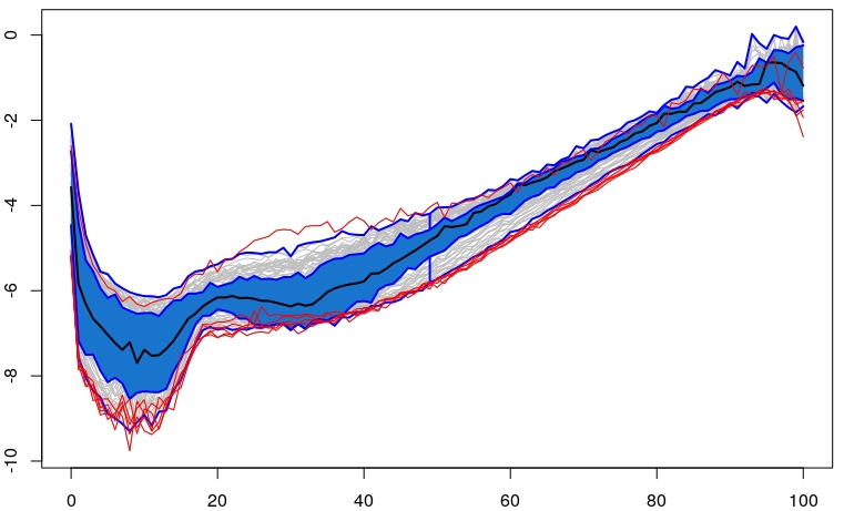
The boxplots for the Berkely growth sets, female and male, are shown in Figure 2. The distributions of the distances in this case are far from the theoretical distribution derived for Gaussian processes. In an attempt to overcome this problem, the parameter is adjusted automatically in order to reduce the Kullback-Leibler divergence between both distributions. The selected values of with this procedure are for the female set and for the male set. In any case, the number of outliers detected is quite large when compared to the sample size.
Female: 3, 8, 10, 13, 15, 18, 26, 29, 42, 43, 48 and 53.
Male: 5, 10, 15, 27, 29, 32, 35 and 37.
But if we look at the estimated density functions corresponding to the distribution of on each set (Figure 3), we can see that these distributions have two modes. In fact, all the curves marked as outliers are the ones that fall into the second mode (whose distance to the mean is greater that the red dotted line). This behavior is similar to the one of the Integrated Squared Error showed in Arribas-Gil and Romo (2014).


5.2 Binary classification
Mahalanobis distance can be used also for classification, classifying each curve through the distance to the nearest mean function, whenever the prior probabilities of the classes are equal. When this is not the case, the rule to classify a coming observation is just to assign it to the population defined by
where stands for the mean functions (for instance, it is used in (Galeano et al., 2015, Section 3.3)). Here we present two different examples of binary classification with same prior probabilities. In order to check the performance of our proposal, we compare it with other classifiers presented below. The name used on the tables for each method is shown between brackets.
- •
Optimal Bayes classifier proposed in Dai et al. (2017) (“OB”). This is a functional extension of the classical multivariate Bayes classifier based on nonparametric estimators of the density functions corresponding to the main coefficients in Karhunen-Loève expansions. Here the curves are projected onto a common sequence of eigenfunctions, and the previous quotient is taken using the densities of these projections. The authors propose three approaches to estimate these densities. We have chosen the implementation which assumes that these densities are Gaussian since, according to their results, it seems to slightly outperform the others. The number of eigenfunctions used for the projections is fixed by cross-validation.
- •
Mahalanobis-based semidistance of Equation (17) proposed in Galeano et al. (2015) (“”).
- •
k-nearest neighbours with and neighbours (“knn3” and “knn5”). In spite of its simplicity, this method tends to show a good performance when dealing with functional data.
Our proposal is denoted as “”. Now the parameter is fixed by cross-validation, for . For heterocedastic problems, we have implemented our binary classifier mimicking an improvement that is usually made in the multivariate context. In that finite setting, given two equiprobable populations with covariance matrices , a curve is assigned to class 1, according to the Quadratic Discriminant classifier, whenever
where the finite dimensional Mahalanobis distance is defined in (1) (see, for instance, Section 8.3.7 of Izenman (2008)). In most cases with multivariate data, classifying with this rule gives better results than merely classifying to class 1 when . In the case of functional data this is just an heuristic improvement. If and are the mean and covariance functions of each class, the standard classifier would assign the curve to the class such that , , is minimum ( stands for the distance when using the covariance function ). Instead, we will classify to class 1 if , and to 0 if not. This constant is computed as , where , , are the ten greater eigenvalues of and respectively.
Cut Brownian Motion and Brownian Bridge
The first problem under consideration is to distinguish between two “cut” versions of a standard Brownian Motion and a Brownian Bridge. By “cut” we mean to take the process on the interval , . We know an explicit expression for the Bayes error of this problem, which depends on the cut point . For the case of equal prior probabilities of the classes, which will be the case here, this Bayes error is given by,
where stands for the distribution function of a standard Gaussian random variable. Since both processes are almost indistinguishable around zero, when . Also when , since then one can decide the class with no error just looking at the last point of the curve.
The trajectories of both processes are shown in Figure 4 and the cut points considered, and , are marked with vertical dotted lines. For each class, 50 samples are drawn for training and 250 for test. The experiment is run 500 times for each cut point, and the trajectories are sampled over an equidistant grid in of size . Table 2 shows the percentages of misclassified curves, as well as the Bayes errors. Our proposal and knn with 5 neighbors seem to outperform the other methods for this problem.

| t | Bayes | OB | knn3 | knn5 | ||
|---|---|---|---|---|---|---|
| 0.75 | 33.9 | 42.5 ( 3.5) | 43.5 ( 2.5) | 46.4 ( 3.2) | 43.2 ( 2.8) | 42.4 ( 2.8) |
| 0.8125 | 30.8 | 40.0 ( 3.7) | 41.9 ( 2.6) | 44.8 ( 3.3) | 41.0 ( 2.8) | 40.1 ( 3.0) |
| 0.875 | 26.9 | 36.1 ( 3.6) | 40.2 ( 2.6) | 42.6 ( 3.7) | 38.0 ( 3.0) | 36.9 ( 3.0) |
| 0.9375 | 20.9 | 32.3 ( 3.1) | 38.0 ( 2.8) | 39.9 ( 3.5) | 33.7 ( 2.7) | 32.5 ( 2.7) |
| 1 | 0.0 | 26.5 ( 2.8) | 35.9 ( 2.9) | 36.0 ( 3.5) | 28.4 ( 2.7) | 27.6 ( 2.7) |
Simulated data
We have implemented also the experimental setting proposed in Dai et al. (2017). The authors consider three different scenarios. For the first two, the curves of both classes and , are drawn from processes
where is a Gaussian variable with zero mean and variance . Function is the th element in the Fourier basis, starting with,
For Scenario A, the coefficients are independent Gaussian variables. For Scenario B they are independent centered exponential random variables. Finally, in Scenario C the processes are
where are the same as in Scenario B and are independent variables with common distribution . Thus, in this latter case the coefficients of the basis expansion are dependent but uncorrelated. The means and the variances of the coefficients , , are changed in order to check the “same” and “different” scenarios for mean and variances. Then always, and is either 0 or . In the same way, the variance of is always and the variance of is either , or . The curves are sampled on 51 equidistant points in .
The prior probabilities of both classes are set to and two sample sizes, 50 and 100, are tested for training. For test we use 500 realizations of the processes. Each experiment is repeated 500 times. The misclassification percentages for all the different scenarios are shown in Table 3. Our proposal is mainly the winner, although in Scenario A it is overtaken by the Optimal Bayes classifier in the case of equal means and different variances. Also knn with 5 neighbors performs better sometimes in the case of different means and equal variances.
| Scenario A (Gaussian) | |||||||
|---|---|---|---|---|---|---|---|
| n | mean | sd | OB | knn3 | knn5 | ||
| 50 | same | diff | 35.9 ( 3.5) | 19.0 ( 4.0) | 47.0 ( 3.1) | 45.6 ( 2.2) | 46.2 ( 2.0) |
| diff | same | 42.3 ( 3.8) | 47.3 ( 6.8) | 43.7 ( 3.7) | 42.9 ( 3.6) | 42.0 ( 3.6) | |
| diff | diff | 29.1 ( 5.0) | 36.4 ( 10.1) | 40.0 ( 5.4) | 39.7 ( 3.0) | 40.0 ( 3.1) | |
| 100 | same | diff | 34.2 ( 3.0) | 9.3 ( 2.1) | 45.8 ( 3.5) | 44.6 ( 1.9) | 45.4 ( 1.8) |
| diff | same | 34.6 ( 4.5) | 45.1 ( 8.2) | 37.0 ( 4.4) | 42.1 ( 3.0) | 41.0 ( 3.0) | |
| diff | diff | 22.0 ( 4.9) | 35.7 ( 11.3) | 34.2 ( 6.2) | 38.3 ( 2.4) | 38.6 ( 2.5) | |
| Scenario B (exponential) | |||||||
| n | mean | sd | OB | knn3 | knn5 | ||
| 50 | same | diff | 24.2 ( 5.2) | 30.2 ( 10.4) | 37.0 ( 6.6) | 37.6 ( 2.6) | 38.0 ( 2.7) |
| diff | same | 41.8 ( 3.9) | 49.1 ( 5.5) | 42.3 ( 4.1) | 38.0 ( 3.4) | 37.2 ( 3.6) | |
| diff | diff | 14.3 ( 4.8) | 31.8 ( 12.8) | 25.1 ( 9.0) | 24.7 ( 3.1) | 25.1 ( 3.5) | |
| 100 | same | diff | 16.9 ( 3.1) | 24.0 ( 9.6) | 28.2 ( 6.1) | 35.3 ( 2.4) | 35.7 ( 2.3) |
| diff | same | 34.5 ( 4.6) | 48.3 ( 5.9) | 36.7 ( 4.2) | 36.5 ( 2.8) | 35.6 ( 2.7) | |
| diff | diff | 7.7 ( 2.9) | 30.1 ( 13.4) | 17.8 ( 6.3) | 21.6 ( 2.4) | 21.8 ( 2.6) | |
| Scenario C (dependent) | |||||||
| n | mean | sd | OB | knn3 | knn5 | ||
| 50 | same | diff | 30.0 ( 5.4) | 33.3 ( 8.1) | 40.1 ( 5.9) | 39.9 ( 2.7) | 39.9 ( 2.7) |
| diff | same | 43.6 ( 4.1) | 48.8 ( 4.8) | 42.9 ( 4.2) | 38.1 ( 3.6) | 37.5 ( 3.8) | |
| diff | diff | 19.9 ( 4.9) | 36.2 ( 11.0) | 30.3 ( 7.7) | 26.4 ( 3.1) | 26.6 ( 3.3) | |
| 100 | same | diff | 21.7 ( 3.0) | 28.0 ( 7.5) | 29.4 ( 5.7) | 37.6 ( 2.4) | 37.5 ( 2.4) |
| diff | same | 38.0 ( 4.3) | 48.8 ( 5.0) | 38.9 ( 3.8) | 36.5 ( 2.7) | 35.6 ( 2.8) | |
| diff | diff | 13.3 ( 3.2) | 34.6 ( 11.0) | 23.2 ( 6.1) | 23.4 ( 2.4) | 23.3 ( 2.4) | |
Acknowledgements
This work has been partially supported by Spanish Grant MTM2016-78751-P. The authors are very grateful to Daniel Estévez for his valuable help with operator theory.
References
- Amini and Wainwright (2012) A. A. Amini and M. J. Wainwright. Approximation properties of certain operator-induced norms on Hilbert spaces. Journal of Approximation Theory, 164(2):320–345, 2012. URL http://dblp.uni-trier.de/db/journals/jat/jat164.html#AminiW12.
- Arribas-Gil and Romo (2014) A. Arribas-Gil and J. Romo. Shape outlier detection and visualization for functional data: the outliergram. Biostatistics, 15(4):603–619, 2014.
- Ash and Gardner (2014) R. B. Ash and M. F. Gardner. Topics in Stochastic Processes: Probability and Mathematical Statistics: A Series of Monographs and Textbooks, volume 27. Academic press, 2014.
- Berlinet and Thomas-Agnan (2004) A. Berlinet and C. Thomas-Agnan. Reproducing kernel Hilbert spaces in probability and statistics. Kluwer Academic, Boston, 2004. ISBN 1-4020-7679-7. URL http://opac.inria.fr/record=b1128469.
- Conway (1990) J. B. Conway. A course in functional analysis, volume 96. Springer Science & Business Media, 1990.
- Cucker and Smale (2001) F. Cucker and S. Smale. On the mathematical foundations of learning. American Mathematical Society, 39(1):1–49, 2001.
- Cucker and Zhou (2007) F. Cucker and D. X. Zhou. Learning theory: an approximation theory viewpoint, volume 24. Cambridge University Press, 2007.
- Cuevas (2014) A. Cuevas. A partial overview of the theory of statistics with functional data. Journal of Statistical Planning and Inference, 147:1–23, 2014.
- Dai et al. (2017) X. Dai, H.-G. Müller, and F. Yao. Optimal bayes classifiers for functional data and density ratios. Biometrika, 104(3):545–560, 2017.
- Galeano et al. (2015) P. Galeano, E. Joseph, and R. E. Lillo. The mahalanobis distance for functional data with applications to classification. Technometrics, 57(2):281–291, 2015.
- Ghiglietti and Paganoni (2017) A. Ghiglietti and A. M. Paganoni. Exact tests for the means of gaussian stochastic processes. Statistics & Probability Letters, 131:102–107, 2017.
- Ghiglietti et al. (2017) A. Ghiglietti, F. Ieva, and A. M. Paganoni. Statistical inference for stochastic processes: two-sample hypothesis tests. Journal of Statistical Planning and Inference, 180:49–68, 2017.
- Gohberg and Goldberg (2013) I. Gohberg and S. Goldberg. Basic operator theory. Birkhäuser, 2013.
- Hsing and Eubank (2015a) T. Hsing and R. Eubank. Theoretical foundations of functional data analysis, with an introduction to linear operators. John Wiley & Sons, 2015a.
- Hsing and Eubank (2015b) T. Hsing and R. Eubank. Theoretical foundations of functional data analysis, with an introduction to linear operators. John Wiley & Sons, 2015b.
- Izenman (2008) A. J. Izenman. Modern multivariate statistical techniques. Regression, classification and manifold learning, 2008.
- Janson (1997) S. Janson. Gaussian Hilbert spaces, volume 129. Cambridge university press, 1997.
- Kato (2013) T. Kato. Perturbation theory for linear operators, volume 132. Springer Science & Business Media, 2013.
- Laha and Rohatgi (1979) R. G. Laha and V. K. Rohatgi. Probability Theory. John Wiley & Sons, New York-Chichester-Brisbane, Wiley Series in Probability and Mathematical Statistics, 1979.
- Lukić and Beder (2001) M. N. Lukić and J. H. Beder. Stochastic processes with sample paths in reproducing kernel Hilbert spaces. Transactions of the American Mathematical Society, 353(10):pp. 3945–3969, 2001. ISSN 00029947. URL http://www.jstor.org/stable/2693779.
- Mahalanobis (1936) P. C. Mahalanobis. On the generalized distance in statistics. Proceedings of the National Institute of Sciences (Calcutta), 2:49–55, 1936.
- Mardia (1975) K. V. Mardia. Assessment of multinormality and the robustness of hotelling’s t 2 test. Applied Statistics, pages 163–171, 1975.
- Penny (1996) K. I. Penny. Appropriate critical values when testing for a single multivariate outlier by using the mahalanobis distance. Journal of the Royal Statistical Society. Series C (Applied Statistics), 45(1):73–81, 1996. ISSN 00359254, 14679876. URL http://www.jstor.org/stable/2986224.
- Reed and Simon (1980) M. Reed and B. Simon. Methods of modern mathematical physics. vol. 1. Functional analysis. Academic New York, 1980.
- Rencher (2012) A. C. Rencher. Methods of multivariate analysis, volume 3 ed. John Wiley & Sons, 2012.
- Rousseeuw and van Zomeren (1990) P. J. Rousseeuw and B. C. van Zomeren. Unmasking multivariate outliers and leverage points. Journal of the American Statistical Association, 85(411):633–639, 1990. doi: 10.1080/01621459.1990.10474920. URL http://www.tandfonline.com/doi/abs/10.1080/01621459.1990.10474920.
- Schölkopf and Smola (2002) B. Schölkopf and A. J. Smola. Learning with kernels: support vector machines, regularization, optimization, and beyond. MIT press, 2002.
- Zuo and Serfling (2000) Y. Zuo and R. Serfling. General notions of statistical depth function. Annals of statistics, pages 461–482, 2000.