Measurement of the Dynamical Structure Factor of a 1D Interacting Fermi Gas

Understanding many-body systems is one of the most important challenges of quantum physics, not only intellectually, but also on how it impacts our ability to develop materials with novel properties. In high dimensions, the cornerstone of our understanding of such systems has been the existence of excitations behaving much like the original individual free particles of which it is comprised. For fermions these are the Landau quasiparticles of Landau’s Fermi liquid theory [1, 2]. In this case, interactions mostly result in the modification of parameters, such as mass.

Very different behavior occurs when the dimensionality of the system is reduced, which reinforces the effects of interactions. In one-dimension, even the physics of nearly free particles may be substantially altered [3]. Because all particles are affected by interactions, in reduced dimensions excitations of the system are collective, while no individual, single particle-like excitations can occur. This leads to a type of physics, known as the Tomonaga-Luttinger liquid (TLL) [4, 5, 6], in which all the excitations are decomposed into collective excitations of charge and spin. As a consequence, the system is critical with correlations decreasing as a power law at zero temperature, and individual excitations fractionalize, decomposing into products of topological excitations carrying spin but no charge (spinons) and charge but no spin (holons) [3]. The physics of such systems is thus controlled by the velocities of the charge and spin collective excitations as well as a dimensionless parameter controlling the power law decay of the correlations. These parameters are directly related to the microscopic interaction in the system [7, 3].

Observing these properties presents considerable challenges. In condensed matter, the power law behaviors attributed to TLL have been seen, in particular, in organic conductors [8], nanotubes [9], and in the conductivity of edge states [10], while spin-charge separation was observed in quantum wires [11]. Further examples of experimental realizations of TLL can be found in [12]. Due to the screened nature of the long-range Coulomb interactions in electronic systems, however, it is difficult to make quantitative comparisons with the TLL theory. In particular, control of interactions has not been previously accomplished. It is thus important to have experimental systems in which such quantitative comparisons can be made. In condensed matter, quantum spin systems provide an excellent route to quantitatively test for TLL [13, 14] but only for interacting bosonic-like systems.

Given their remarkable degree of control of lattice structure and interactions [15], cold atoms provide a promising, complementary route to tackle TLL physics. The contact nature of interactions in cold atoms, and their control via a Feshbach resonance [16] enables detailed comparison between the theoretical predictions of TLL and experiment. The possibility of measuring the dynamical structure factors of charge and spin provides a check that collective excitations indeed control the entire excitation spectrum. Realizing these measurements, however, has not proven to be easy. For bosonic systems, quasi-long range behavior of correlation functions consistent with TLL predictions have been observed for optical lattices [17] and for atom chips [18], and the sound velocity connected to TLL physics [19] and the dynamical structure factor [20] were recently measured. For fermionic systems, the dynamical structure factor was probed for SU(N) fermions [21], but due to the absence of a Feshbach resonance, a detailed analysis of the excitation spectrum as a function of the interaction strength has been missing.

In this paper, we use Bragg spectroscopy [22, 23] to measure the dynamical structure factor $S(q,\omega)$ of the density (“charge”) mode of a one-dimensional (1D) Fermi gas of fermionic ⁶Li whose repulsive $s$-wave interactions are broadly tunable. Bragg spectroscopy, which employs two-photon stimulated transitions, is a sensitive method to detect density fluctuations, and thus $S(q,\omega)$ in cold atom systems. Our measurement of $S(q,\omega)$ for $q<k_{\textrm{F}}$, where $k_{\textrm{F}}$ is the Fermi momentum, agrees well with the TLL theory when using the local density approximation to account for the density inhomogeneity of the trapped gas, thus providing the first exploration of such physics with cold atomic fermions with tunable interactions.

The 1D experiment of Ref. [21] employed Bragg spectroscopy to measure the low-energy energy excitation spectra of the density mode of a 1D Fermi gas with a tunable number of spin components. Bragg spectroscopy has also been used to measure the dynamical structure factor in 3D for both the spin and density excitations of a strongly interacting Fermi gas at high momentum, where $q\gg k_{\textrm{F}}$, [24], and more recently, the charge excitation spectrum for $q\lesssim k_{\textrm{F}}$ [25].

The two lowest hyperfine sub-levels ($|F=1,m_{F}=1/2\rangle$ and $|F=1,m_{F}=-1/2\rangle$) of ⁶Li constitute a quasi-stable, pseudo-spin-1/2 system, which we label as $|\penalty\uparrow\penalty\rangle$ and $|\penalty\downarrow\penalty\rangle$, respectively. The three-dimensional $s$-wave scattering length, $a$, for states of opposite spin projection can be tuned from $a=0$ at 528 G, to $a\simeq 400$ $a_{0}$ at 606 G, where $a_{0}$ is the Bohr radius [26]. Beyond this repulsive interaction strength, however, the “upper branch” of the Feshbach resonance becomes unstable to the formation of deeply bound dimers [27].

The apparatus and some of the methods used in this experiment have been described previously [27, 28]. We focus here on the primary differences. The atoms are loaded into a crossed beam optical trap formed from three mutually orthogonal infrared (IR) laser beams. These beams are retroreflected, but the polarization of each retroreflected beam is rotated by 90^∘ to form a trap without a lattice. After loading this trap, we measure the total number of atoms and their temperature to be $1.4\times 10^{5}$ and 0.05 $T_{\textrm{F}}$, respectively, where $T_{\textrm{F}}$ is the Fermi temperature of each spin state assuming no interactions. We then increase the depth of the trap and rotate the polarization of the retroreflected beams to form a 3D optical lattice with a lattice depth $V_{\textrm{L}}=7E_{\textrm{r}}$, where $E_{\textrm{r}}=h^{2}/(2m\lambda^{2})$ is the recoil energy, $h$ is Planck’s constant, $m$ is the atomic mass, and $\lambda=1,064$ nm is the wavelength of the light. During this process, we also adjust the scattering length to desired final value before the lattice depth reaches $V_{\textrm{L}}=2.5E_{\textrm{r}}$. We superimpose a blue-detuned (532 nm), non-retroreflected laser beam along each axis to partially compensate the overall confining envelope of the infrared beams [29, 27]. The intensities of the compensating beams are adjusted to flatten the confining potential and to tune the central density in the lattice to be near one atom per site, $n\simeq 1$, for each interaction strength. Previous measurements showed that the atoms formed a Mott insulator for $a\gtrsim 250a_{\textrm{o}}$ at $V_{\textrm{L}}=7E_{\textrm{r}}$ [28]. The small variation of density for different interactions is an important feature of our experiment.

We then slowly turn off the compensating green beams and the vertical IR beam while simultaneously increasing the intensity of the two remaining lattice beams to form a 2D lattice with $V_{\textrm{L}}=15E_{\textrm{r}}$. The 2D lattice creates a bundle of nearly isolated 1D tubes, characterized by axial and radial harmonic frequencies of $\omega_{\textrm{z}}=(2\pi)1.3$ kHz, and $\omega_{\perp}=(2\pi)198$ kHz, respectively. The final total atom number is $N=1.1\times 10^{5}$. The total number of atoms in the central tube, $N_{m}$, is nearly independent of $a$ for stronger interactions, but is somewhat larger for smaller $a$. By performing an inverse Abel transform on column density images we determine the 3D density distributions, and find that $N_{m}$ varies from 55, at larger $a$, to 70 for an ideal gas. The most probable atom number per tube is between 37 and 40 for all interactions. Taking $N_{m}=60$ gives $k_{B}T_{F}=1.9~\mu$K for each spin-state, which is much less than $\hbar\omega_{\perp}=9.5~\mu$K.

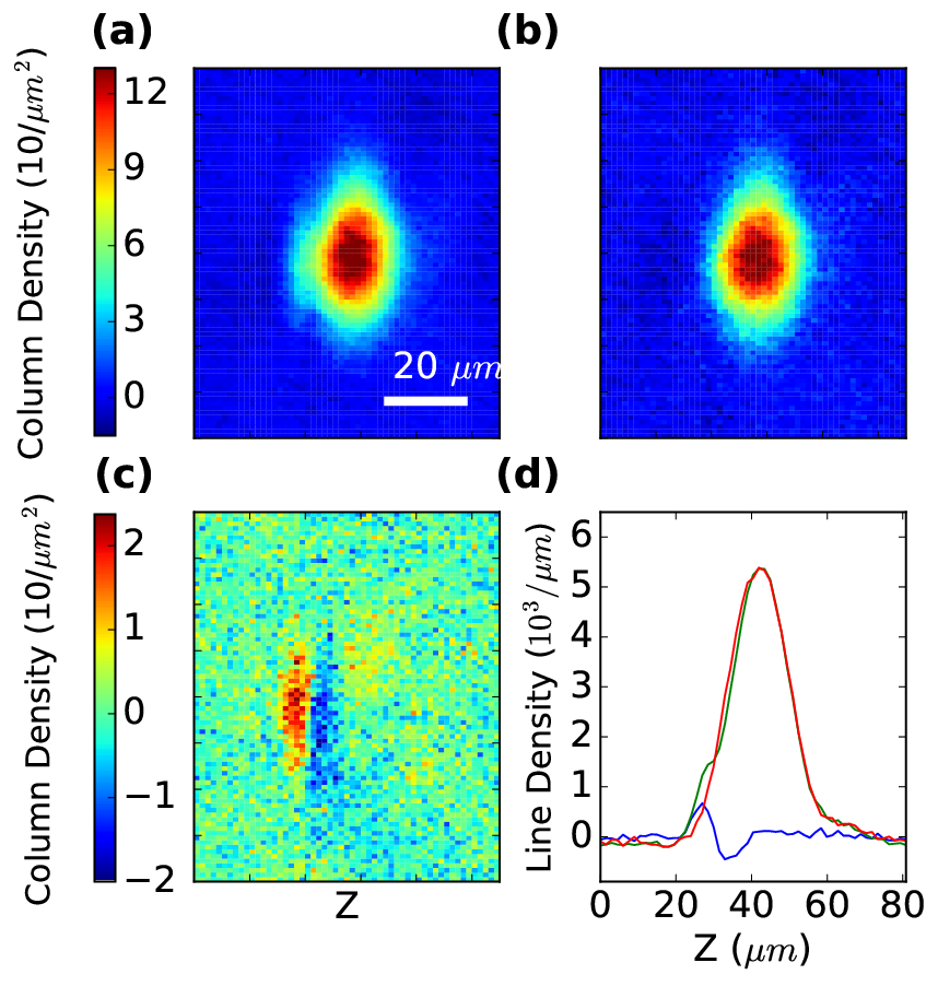
Bragg spectroscopy employs two laser beams, with wavevectors $\mathbf{k_{1}}$ and $\mathbf{k_{2}}$ and frequency difference $\omega$. They propagate with an angle $\theta$ between them and intersect the atoms symmetrically about a line perpendicular to the tube ($z$) axis, and thus possess a net momentum along the z-direction. These beams drive a stimulated two-photon transition that couples the ground state to an excitation of frequency $\omega$ and z-component of momentum $q=|\mathbf{k_{1}}-\mathbf{k_{2}}|=2k\sin(\theta/2)$, where $k=|\mathbf{k_{1}}|=|\mathbf{k_{2}}|$. We fix the angle $\theta/2\simeq 4.5^{\circ}$ such that $q/k_{\textrm{F}}\simeq 0.2$ for a central tube filling of $N_{m}=60$.

The Bragg beams are detuned by 14 GHz blue of the D₂ transition in ⁶Li in order to minimize the rate of spontaneous emission. Since the detuning is large compared with the 76 MHz splitting between the $|\uparrow\rangle$ and $|\downarrow\rangle$ states, the signal is sensitive only to density excitations and not to spin. The Bragg beams are pulsed on for 300 $\mu$s, which is less than half the axial period, but long compared with $\omega^{-1}$, conditions that both simplify the analysis [23] and minimize the pulse-time broadening. The optical lattice beams are switched off immediately following the Bragg pulse. After 150 $\mu$s of time of flight, we image the column density distribution of both states using phase-contrast polarization imaging [32] with a probe detuning of 33 MHz red of the $|\downarrow\rangle$ imaging transition (and 110 MHz red of the $|\uparrow\rangle$ transition). By repeating the experiment without Bragg beams, we record a reference image that we subtract from the signal image obtained with the Bragg beams present, as shown in Fig.  1. These column density images are integrated in the direction transverse to the tube axis to obtain axial line densities shown in Fig. 1(d). The integral under the positive part of the line densities are proportional to the total momentum transferred by the Bragg beams, and is what we define as “signal”.

We checked that the Bragg signal is in the linear response regime by varying the Bragg beam intensity, while fixing the pulse duration. In this regime, the rate of stimulated Bragg transitions should depend quadratically on the laser intensity (assumed equal for each beam). As shown in Fig. 2, an intensity per beam of less than 55 mW/cm² ensures that the momentum transfer is in the linear response regime over the entire range of interaction strengths accessed in the experiment. We fix the intensity at this value.

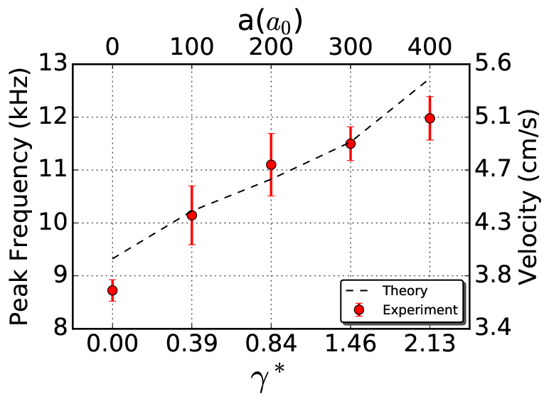
The Bragg spectra for five values of the interaction parameter are presented in Fig. 3. Each data point corresponds to an average of 20-30 experimental runs for each value of $\omega$ and fixed $q$. The full-width at half maximum of these spectra range from 9 kHz for a noninteracting gas to 11 kHz for the most strongly interacting one. These spectral widths are large compared to the pulse-time broadening of 3 kHz. The spectra are empirically found to fit well to a skew normal distribution (convolution of a Gaussian with the error function). The most probable value of $\omega$ may be obtained from the fitting parameters for each interaction, and these are plotted in Fig.  4. The most probable frequency increases with interaction strength until $a=400a_{0}$. We notice heating and atom loss beyond this interaction, quite probably due to three-body recombination from the unstable upper branch during the transition from the 3D to 2D lattice. In contrast, we observe no atom loss for $a$ between 0 and 400 $a_{0}$.

In the linear response regime, the experimentally measured momentum transfer for each $q$ and $\omega$ is proportional to $S(q,\omega)-S(-q,-\omega)$, where the second term accounts for inverse Bragg scattering: absorption by beam 2 and stimulated emission by beam 1 [23]. The second term will be small compared to the first when $k_{B}T\ll\hbar\omega$ [33, 23], and in this case, the measured Bragg signal is proportional to $S(q,\omega)$.

In order to compare with theory, an inverse Abel transform is applied to the measured column densities (without a Bragg pulse) to obtain the distribution of atom number per tube at each interaction strength. Using the local density approximation (LDA) we split each tube into about a hundred pieces of length $dz$ with constant density $n(z)$, calculate the dynamic structure factors independently for each piece, and sum them together to get the momentum transfer for one tube. As momentum is an additive quantity, we repeat this procedure for each tube in the lattice, summing the individual momentum transfers into the resulting total momentum transfer.

For a homogeneous Fermi gas, the dynamic structure factor is:

where $\chi$ is the dynamic susceptibility [34]. The TLL theory [3] states that at small $q$ the susceptibility is dominated by a collective charge mode, whose velocity has a very precise interaction dependence that can be computed exactly with known interactions [35]. For a homogeneous system at zero temperature and small $q$, the susceptibility has a resonance at $\omega=uq$ giving direct and convenient access to the velocity of charge excitations. Thus, for weak interactions, Eq. 1 may be used to calculate the structure factor, but in this case, substituting the speed of sound $u$ obtained from Bethe Ansatz [35] for the Fermi velocity to account for the shift in the resonance. The velocity $u$ may be calculated exactly as a function of interaction. More details of our theoretical analysis are available in the Supplemental Materials ¹¹ 1 See Supplemental Material [URL] for additional details of our theoretical analysis, which includes Ref. [40]..

We use this procedure to calculate the structure factor for a temperature of 200 nK, and compare with the experimental data, as shown in Fig. 3. The only adjustable parameter is the overall scaling of the excitation. The agreement between the calculated lineshape with the experimental one validates our method to account for the sources of broadening, and shows that the experiment gives direct access to the interaction dependence of the velocity. The peaks of the experimental excitation spectra for each interaction are plotted in Fig. 4 together with the theoretical result. The agreement between the measured and computed interaction dependence of the velocity is very good and provides the first experimental test of the change in velocity of the collective excitation of a 1D Fermi gas vs. interactions.

We also attempted to measure the dynamical structure factor of the spin mode by adjusting the detuning of the Bragg laser to be negative for one spin state, while positive for the other [27]. Since the two optical transitions are separated by only 76 MHz, however, we were unable to observe a Bragg signal without destroying the sample with excessive spontaneous emission from the excited 2P state. It may be possible to observe a spin-dependent Bragg signal in the future by detuning from the 3P excited state instead, as the rate of spontaneous emission is reduced by the ratio of linewidths, which is a factor of 8 in this case [37]. Such a measurement will thus give full access to the two collective modes controlling the physics of the interacting fermionic system. Furthermore, it would be interesting to couple such measurements with those of the single particle excitation spectrum, e.g. by momentum resolved RF spectroscopy [38, 39], to establish the link between the single particle spectrum and the collective modes predicted by TLL.

In conclusion, we have measured the dynamic response of a one-dimensional two-component fermionic system using Bragg spectroscopy and find good agreement with TLL theory for the collective charge mode. The ability to adjust the interaction strength via a Feshbach resonance enables future studies such as a direct observation of spin-charge separation, the dynamic response for high q excitation that goes beyond the Luttinger liquid theory, or possibly a system with p-wave interactions for a single spin state.

References

- [1] T. Giamarchi, Quantum Physics in One Dimension (Oxford University Press, Oxford, 2004)
- [2] X. W. Guan, M. T. Batchelor, and C. Lee, Reviews of Modern Physics 85, 1633 (2013)
- [3] J.-S. Caux and P. Calabrese, Physical Review A 74, 031605 (2006)