Computing performability measures in Markov chains by means of matrix functions Note: This research has been partially supported by the ISTI-CNR project “TAPAS: Tensor algorithm for performability analysis of large systems”, by the INdAM/GNCS project 2018 “Tecniche innovative per problemi di algebra lineare”, and by the Region of Tuscany (Project “MOSCARDO - ICT technologies for structural monitoring of age-old constructions based on wireless sensor networks and drones”, 2016–2018, FAR FAS).
Abstract
We discuss the efficient computation of performance, reliability, and availability measures for Markov chains; these metrics — and the ones obtained by combining them, are often called performability measures.
We show that this computational problem can be recasted as the evaluation of a bilinear form induced by appropriate matrix functions, and thus solved by leveraging the fast methods available for this task.
We provide a comprehensive analysis of the theory required to translate the problem from the language of Markov chains to the one of matrix functions. The advantages of this new formulation are discussed, and it is shown that this setting allows to easily study the sensitivities of the measures with respect to the model parameters.
Numerical experiments confirm the effectiveness of our approach; the tests we have run show that we can outperform the solvers available in state of the art commercial packages on a representative set of large scale examples.
Keywords:
Markov chains, Performance measures, Availability, Reliability, Matrix functions- CTMC
- Continuous Time Markov Chain
- MRP
- Markov Reward Process
- SPN
- Stochastic Petri Net
- PEPA
- Performance Evaluation Process Algebra
1 Introduction
Performance and dependability models are ubiquitous [29] in design and assessment of physical, cyber or cyber-physical systems and a vast ecosystem of high level formalisms has been developed to enhance the expressive power of CTMC. Examples include dialects of SPN such as Stochastic Reward Nets [29], Queuing networks [4], dialects of PEPA (PEPA) [18], and more. High level formalisms are to CTMC what high level programming languages are to machine code; in this setting, performance and dependability measures are usually defined following high level formalisms primitives. Once model and measures have been defined, automatic procedures synthesize, transparently to the modeler, a CTMC and a reward structure on it, producing a MRP (MRP), and the measures of interest are derived as a function of the reward structure.
The main contribution of this paper is to show that the computation of these measures can be recasted in the framework of matrix functions, and therefore enable the use of fast Krylov-based methods for their computation. In particular, we provide a translation table that directly maps common performability measures to their matrix function formulation. Moreover, our approach is easily extendable to other kinds of measures. Matrix functions are a fundamental tool in numerical analysis, and arise in different areas of applied mathematics [17]. For instance, they are used in the evaluation of centrality measures for complex networks [12], in the computation of geometric matrix means that find applications in radar [5] and image processing techniques [14, 25], as well as in the study and efficient solution of system of ODEs [2, 19] and PDEs [31].
Many numerical problems in these settings can be rephrased as the evaluation of a bilinear form , where is an assigned (matrix) function, a matrix, and and vectors. Often, the interest is in the approximation of for a specific choice of the arguments , and so an explicit computation of is both unnecessary and too expensive.
Therefore, one has to resort to more efficient methods, trying to exploit the structure of when this is available. For instance, in [13] the authors describe an application to network analysis that involves a symmetric (the adjacency matrix of an undirected graph), and they propose a Gauss quadrature scheme that provides guaranteed lower and upper bounds for the value of . Other approaches exploiting banded and rank structures in the matrices, often encountered in Markov chains, can be found in [6, 21]. These properties have already been exploited for the steady-state analysis of QBD processes [7, 8].
We prove that performability measures defined in CTMCs can be rephrased in this form as well. In particular they can be written as , where is the infinitesimal generator of the Markov chain (also called Markov chain transition matrix), and , and are chosen appropriately. CTMC arise when modeling the behavior of resource sharing systems [4], software, hardware or cyber-physical systems [29], portfolio optimization [32], and the evaluation of performance [4], dependability [3, 28] and performability [23] measures that we are going to rewrite as bilinear forms . These models are obtained with different high-level formalism; however, all of them are eventually represented as CTMCs.
A simple example, which is analyzed in more detail in Section 6.1, can be constructed by a set of states, numbered from to , assuming that we can transition from state to with an exponential distribution with parameter , and from to with rate . Pictorially, this can be represented using the following reachability graph:
In this case, the infinitesimal generator matrix has the following structure:
where is nonzero if and only if there is an edge from state to .
Rephrasing performability measures using the language of matrix functions opens also new direction of research regarding how structures that are visible at the level of these high level formalism are reflected into the CTMC infinitesimal generator, and then can be exploited to enhance measures’ evaluation.
The paper is structured as follows. We start with a brief discussion of modeling and matrix function notations in Section 2.1. The main contribution is presented in Section 3, where we give a dictionary for the conversion of standard performance, dependability and performability measures in the parlance of matrix functions.
Using this new formulation, we present a new solution method in Section 4, and we demonstrate in Section 5 that this framework can be used to describe in an elegant and powerful form the sensitivity of the measures, which is directly connected to the Frechét derivative of at . We show that, when an efficient scheme for the evaluation of is available, the sensitivity of the measures can be estimated at almost no additional cost.
Finally, we perform numerical tests on three relevant case studies in Section 6. The new method is shown to be efficient with respect to state-of-the-art solution techniques implemented in commercial level software tools. We also test our method to compute the sensitivity of measures as described in Section 5. The numerical experiments demonstrate that the computation requires less than twice the time needed to simply evaluate the measure.
To enhance readability, mathematical details are presented in the appendix. In particular, a brief discussion of the spectral properties of that are most relevant for our study is offered in appendix A.2; then, we give a summary of the currently available methods to compute performability measures in appendix A.3 and standard notions about matrix functions in appendix A.4. Details about the translation to matrix functions are presented in appendix Appendix B, where we provide a proof of the two main lemmas, Lemma 2.2 and Lemma 2.3, and we present additional remarks about their application.
2 Performability measures as matrix functions
2.1 Model and notation
We recall that Markov chains are stochastic processes with the memory-less property, that is the probability of jumping from state to state after some time depends only on and , and not on the previous history. We consider CTMC where the state space is finite so, without loss of generality, we assume it to be .
In addition, we assume that the probability of jumping from to is distributed with a given exponential rate , so that we may define a matrix with entries
where we set for any . With this definition, given a certain initial probability distribution , where the entry with index corresponds to the probability of being in the state , the probability at time can be expressed as
The stationary (or steady-state) distribution , that is the limit of for is guaranteed11 1 The uniqueness and existence of is discussed in appendix A.1 in further detail. to exist if the process is irreducible. If the process has absorbing states, then the stationary distribution might not exists or not be unique; in this case, it is typically of interest to study the transient behavior of the process.
From the modeling perspective, the steady-state distribution describes the long-term behavior of a system. However, when assessing the performance and reliability of processes modeling real-world phenomena, it is essential to characterize the transient phase as well, that is the behavior between the initial configuration and the steady-state. Moreover, the transient state is relevant also when is reducible, even though the steady-state distribution is not well-defined in this case.
In practice, if the system has a large number of states, computing at some time is not the desired measure; it is far more interesting to obtain concise information by “postprocessing” in an appropriate way. Note that, in this framework, it is expected that depends on the initial choice of , so that is an important parameter that needs to be known.
Let us make an example to further clarify this concept. Consider a Markov chain , with infinitesimal generator , modeling a publicly available service. Assume that we can partition the states in two sets and . The first contains the states where the system is online (“up”), whereas the second the ones where the system is offline (“down”). Up to permuting the states, we can partition the matrix according to this splitting:
In a certain interval of time , we would like to know how long the system is expected to stay online. This can be measured by computing integral
We note that , where is the vector with ones in the states of , and otherwise, and denote the usual scalar product. This is what we call the uptime of the system in . If the set is the set of absorbing states, then this measure coincides with the reliability of the system.
This is an instance of a broader class of measures that belong to the field of performance, availability and reliability modeling. In the literature, the terms performance and availability refer to measures depending on the steady-state, whereas reliability concerns the transient phase of a reducible chain. Measures combining performance and availability (or reliability in the reducible case) are called performability measures [22].
This paper is concerned with the efficient computation of such measures, which will be obtained by rephrasing the problem as the evaluation of a bilinear form induced by a matrix function.
The main tool used to devise fast algorithms for the evaluation of these measures is recasting them as the computation of matrix functions. Informally, given any square matrix and a function which can be expanded as a power series, a matrix function is defined as:
The most well-known example is the case , where . Another function of interest in this paper is . The definition holds in a more general setting, as discussed in appendix A.4.
Let us fix some notation. We denote by a fixed weight vector of elements, so that is a process whose value at time corresponds to entry of index in . In most cases, will be the reward vector, containing a “prize” assigned for being a certain state. We shall give two definitions of reward measures, to simplify the discussion of their computation later on.
Definition 2.1.
Let be a reward vector, and a Markov chain with infinitesimal generator . Then, the number is called instantaneous reward measure at time , and is denoted by . Similarly, the number
is called cumulative reward measure at time .
Note that both definitions depend on the choice of the reward vector . This dependency is not explicit in our notation to make it more readable — in most of the following examples the current choice of will be clear from the context. Occasionally, we will make this dependency explicit by saying that a measure is associated with a reward vector .
Intuitively, the instantaneous reward measures the probability of being in a certain set of states (the non-zero entries of ), weighted according to the values of the components of . The cumulative version is averaged over the time interval . For instance, for the uptime we had .
In the remaining part of this section, we show that reward measures can be expressed as , for a certain reward vector and an appropriate function .
The next result is the first example of this construction, and concerns instantaneous reward measures.
Lemma 2.2.
Let be an instantaneous reward measure associated with a vector and a Markov process generated by and with initial state . Then, , with
Proof.
The equality follows immediately by the relation . ∎
A similar statement holds for the cumulative reward measure.
Lemma 2.3.
Let be an cumulative reward measure, as in Definition 2.1. Then, , with
Proof.
The proof of this Lemma is given in Appendix B. ∎
3 Translation of performability measures into matrix functions
The purpose of this section is to construct a ready-to-use dictionary for researchers involved in modeling that can be used to translate several known measures to the matrix function formulation with little effort. This is achieved by applying some theoretical results which, to ease the reading, are discussed in Appendix B. Following these results, one can derive analogous formulations for additional performability measures.
For many measures, it is important to identify a set of states that correspond to the online or up state: when the system is in one of those states then it is functioning correctly. To keep a uniform notation, we refer to this set as . Its complement, the offline or down states, will be denoted by . In the case of reducible Markov chains, the set of “down” states typically coincides with the absorbing ones. This hypothesis is necessary for some measures (such as the mean time to failure) in order to make them well-defined.
Clearly, the actual meaning of being “up” or “down” may change dramatically from one setting to another; but the computations involved are essentially unchanged — and therefore we prefer to keep this nomenclature to present a unified treatment. A summary of all the different reformulations in this section, with references to the location where the details are discussed, is given in Table 1.
3.1 Instantaneous reliability
We consider the case of a reducible chain, with a set of absorbing states (the “down” states). We are concerned with determining the probability of being in an “up” state at any time . This measure is called instantaneous reliability.
This measure can be computed considering the probability of being in a state included in the set , i.e.,
where is the vector with components on the indices in , and zero otherwise. Therefore, this availability measure is rephrased in matrix functions terms as .
In the same way, we may define the measure , which is the probability of being in “down” state at the time . Notice that this can also be expressed in matrix function form by .
3.2 Instantaneous availability
In irreducible Markov chains, the instantaneous availability is the analogue of the reliability described in the previous section, that is, we measure the probability of the system being “up” at any time . We note that, mathematically, the definition of reliability and availability coincide but the former term is considered when dealing with reducible Markov chains, whereas the latter is employed for irreducible ones. In particular, the availability can be expressed in matrix function form as follows: .
When the states in correspond to the working state of at least components out of , this measure is often called the -out-of- availability of the system.
| Measure | Function | Reward vector | Matrix | Reference |
|---|---|---|---|---|
| Inst. reliability | Section 3.1 | |||
| Inst. availability | Section 3.2 | |||
| MTTF | Section 3.3 | |||
| Exp. # failures | Section 3.4 | |||
| Uptime | Section 3.5 | |||
| Average clients | Section 3.6 |
3.3 Mean time to failure
We consider the expected time of failure for a model. This measure is relevant for devices which fail, and cannot be repaired. In particular, it is possible to exit from states in , but one can never go back again: the Markov chain is reducible and is a set of absorbing states. The average time needed to exit can be expressed as the average time that one spends inside . In probabilistic terms,
where denotes the component of index in the vector . For this measure to be finite, it is necessary that all the states inside of have zero probability in the steady-state. This can be rephrased using as follows:
Here, one could be tempted to apply Lemma 2.3 directly, but this is not feasible. In fact, taking the limit of to for gives , which has a pole at , and is always singular. However, one can notice that, for , we have where is the vector of initial conditions restricted to the indices in . Therefore, we can apply Lemma 2.3 and take the limit of to obtain:
which can be written simply as . The matrix is invertible22 2 See Lemma A.4, its inverse is nonnegative [24], and therefore .
The same measure is often restricted to the interval . In this case, we may write
We note that this formulation is well-defined even when goes to infinity. In fact, a direct application of Lemma 2.3 yields
and this function does not have a pole in . Nevertheless, also in this case it holds true that , and this gives a reduction in the size of the matrix whose exponential needs to be computed, so this reformulation may be convenient in practice.
3.4 Expected number of failures
We consider a system partitioned as usual in up and down states (denoted by and ). We are interested in computing the expected number of transitions between a state in to a state in (the number of failures).
If we consider two states and , then the expected number of transitions from to in a certain time interval can be expressed as
When considering two sets of states, and , this can be generalized to the expected number of transitions from to by
where , and are the probability distributions restricted to the states in .
3.5 Uptime
The uptime measure determines the expected availability of a system in a time interval , for an irreducible Markov chain. To this end, we need to partition the states in online and offline, and to compute the integral
We note that this is the integral analogous of the instantaneous availability defined for irreducible systems in Section 3.2. In fact, a straightforward computation shows that
as predicted by Lemma 2.3. We notice that this measure is not well-defined if we let go to infinity, since for every irreducible Markov chain , and therefore the limit of needs to be infinite, because the integrand is not infinitesimal.
3.6 Average number of clients
We now discuss a measure which is specifically tailored to a model but, with the proper adjustments, can be made fit a broad number of settings. Assume we have a Markov chain that models a queue (which might be at some desk serving clients, a server running some software, or similar use cases). The state of is the number of clients waiting in the queue, and we assume a maximum number of slots. At any time, the process can finish to serve a client with a rate , or get a new client in the queue with rate .
We are interested in the expected number of clients in the queue at time , or at the steady state (that corresponds to ). In the two cases, this measure can be expressed as
where as usual we denote by the limit of to the steady-state. It is clear that, since , we can express as the bilinear form . It is interesting that one can express the steady state probability in matrix function form as well. In fact, if we define as the function equal to at and elsewhere, we can express33 3 This is proven in Lemma B.2. as .
4 Efficient computation of the measures
In view of the analysis of Section 3, we are now aware that several measures associated with a Markov process are in fact computable by evaluating , for appropriate choices of and of the matrix function . A straightforward application of standard dense linear algebra methods to compute usually has complexity , where is the size of the matrix , which in this case is the number of states of the underlying Markov chain.
It is often recognized in the literature that the matrix generating the Markov chain is structured, and allows for a fast matrix vector product . Typically, we can expect this operation to cost flops, where is the number of states in the Markov chain. In this section we propose to leverage well established Krylov approximation methods for the computation of , which in turn yields an algorithm for evaluating in linear time and memory. Similar ideas and techniques can be found in exponential integrators, see [16].
Here we recall only the essential details needed to carry out the scheme, and we refer to [15] and the references therein for further details. We now focus on the computation of , ignoring . Once this is known, can be obtained in flops through a scalar product.
4.1 Krylov subspace approximation
The key ingredient to the fast approximation of is the so-called Arnoldi process, the non-symmetric extension of the Lanczos scheme. From now on, we assume without loss of generality that . Consider the Krylov subspace of order generated by and as
Assuming no breakdown happens, the Arnoldi scheme provides an orthogonal basis for this space that satisfies the relation:
where is an upper Hessenberg matrix, a scalar, a vector, and the -th column of the identity matrix. This relation is often used in the description of the classical Arnoldi method, and can be employed to iteratively and efficiently construct the basis . We refer the reader to [11] for further details. This can be used to retrieve an approximation of by computing . This approximation has several neat features, among which we find the exactness properties: the approximation is exact if is a polynomial of degree at most . We would like to characterize how accurate is this approximation for generic function. To this aim, we introduce the following concept.
Definition 4.1.
Given a matrix , the subset of the complex plane defined as
is called the field of values of .
The above set is easily seen to be convex, and always contain the eigenvalues of . Whenever is a normal matrix (for instance, when is symmetric), then the set is the convex hull of the eigenvalues. For non-normal matrices, this set is typically slightly larger, but the following relation holds:
where is the spectrum, i.e., the set of eigenvalues, of . so in particular the set is not unbounded and, in the Markov chain setting, it is typically to estimate to obtain a rough approximation of its radius.
Lemma 4.2.
Let be a function defined on the field of values of , and a polynomial approximant of such that on . Then,
Proof.
This inequality follows immediately from the well-known Crouzeix inequality (sometimes called Crouzeix conjecture, since the bound is conjectured to hold with in place of ). See, for instance, [9]. ∎
A straightforward implication of the above result is that if is a degree approximant to and on a domain containing , then can be bounded by writing and using the exactness property:
We know, for instance by Weierstrass’ theorem, that polynomials approximate uniformly continuous functions on a compact set, so this alone guarantees convergence of the scheme. However, it tells us very little about the convergence speed. It turns out that, for many functions of practical use that have a high level of smoothness (such as ), the convergence is fast.
When the dimension of the space increases, the orthogonalization inside the Arnoldi scheme can become the dominant cost in the method. For this reason, it is advisable to employ restarting techniques. These aim at stopping the iteration after becomes sufficiently large, and consider a partial approximation of the function . Then, the residual is approximated by restarting the Arnoldi scheme from scratch. The efficient and robust implementation of this scheme is non-trivial; we use the approach developed in [15], to which we refer the reader for further details on the topic.
4.2 Approximation of exponential and
After running the Arnoldi scheme, we are left with a simpler problem: we need to compute , where is a small matrix. In our case, we are interested in the functions
The literature on the efficient approximation of the matrix exponential is vast; the most common approach for is to use a Padé approximation scheme coupled with a scaling and squaring technique, which is the default method implemented by MATLAB through the function expm; see the discussion in [17] for the optimal choice of parameters for the scaling phase and the approximation rule. Then, one can consider the rational approximant to obtained using the Padé scheme with order , let us call it , and so we have
The latter matrix power can be efficiently computed by steps of repeated squaring, and the evaluation of the rational function requires matrix multiplications and one inversion. The order has to be chosen depending on the level of squaring (i.e., on the value of ), and is an integer between and (parameter tuning for optimal performance and accuracy can be a tricky task, so we suggest to either refer to [17] or to rely on the MATLAB implementation of expm).
Concerning the computation of , we use a trick widely used in exponential integrators. In particular, we propose to recast the problem as the computation of a matrix exponential, by exploiting the following known result from the framework of exponential integrators, whose proof can be found in [2, Theorem 2.1].
Theorem 4.3.
Let be any square matrix, and . Then, the following relation holds:
The above result tells us that the action of on a vector can be obtained by computing the action of a slightly larger matrix on the vector padded with a final zero. Even when the norm of is large, the techniques in [15] allow to accurately control the approximation error.
4.3 Incorporating restarting
In practice, the dimension of the Krylov space needed to achieve a satisfactory accuracy might be high, and therefore a more refined technique is needed to achieve a low computational cost. One of the most efficient techniques is to incorporate a restarting scheme: we stop the method after the dimension of the space reaches a certain maximum allowed dimension, obtaining an approximation of low-quality. Then, we restart the method to approximate , i.e., the residual. The procedure is then repeated until convergence.
5 Sensitivity analysis
Performance and dependability models are often parametric, in the sense that some transition rates can be functions of some parameter . As described in [26], the sensitivity analysis is the study of how the measures of interest vary at changing .
5.1 A motivation for sensitivity analysis
During the design phase, a key requirement is to isolate the set of parameters that most influence the behavior of the system. This can guide optimization to the design. In particular, this allows to investigate the return of an investment aimed at changing some components, in terms of enhanced reliability and/or availability. When the budget for developing a new product is limited, this is of paramount importance.
Moreover, real world parameters come from actual (physical) measurements and therefore might be affected by measure errors of different orders of magnitude, in particular for cyber-physical systems. Sensitivity analysis can guide the effort in collecting the most relevant parameters with high precision and the other parameters with acceptable precision.
Another setting where sensitivity analysis plays a relevant role is the modeling of complex systems, where certain aspects of the system behavior are often abstracted away because the time scale at which they appear is considered too fine (avoiding stiffness) or in order to maintain a reasonable level of complexity within the model itself (state space explosion avoidance). In particular, a hierarchical modeling strategy [28] may be adopted: specific system components are modeled in isolation, measures are defined on them and the numerical value obtained evaluating the measures are used as parameters for the overall system model. The hierarchical strategy can be employed whenever the system logical structure presents a (partial) order among components and can involve several layers. Establishing to which extent each layer is sensitive to those parameters that come from an underlying layer enhances and guides modeling choices.
5.2 Sensibility analysis and Frechét derivatives
We are interested in bounding the first order expansion of a measure when the infinitesimal generator changes along a certain direction. Let be a performability measure of a system with matrix depending on a parameter in a smooth way. We want to determine a real positive number such that:
This characterizes the amplification of the changes in the system behavior when the parameter changes. If depends smoothly on then we can expand it around :
From now on, by a slight abuse of notation, we will write in place of , meaning that the bound is correct up to the second order terms in norm. A straightforward computation yields the following result.
Lemma 5.1.
Let a matrix with a dependency on around a point , and let . Then, we have
where is the Frechét derivative of the matrix function .
Even more interestingly, there exists a simple strategy (presented, for example, in [17]) to compute the Frechét derivative along a certain direction by making use of block matrices. Specializing it to our case yields the following corollary.
Corollary 5.2.
Let a matrix with a dependency on around a point , and let . Then, we have
where the vectors are partitioned accordingly to the block matrix.
Proof.
The result is an immediate consequence of [17, Theorem 4.12]. ∎
In view of the above result, if we are given an efficient method to evaluate , the sensitivity with respect to a certain perturbation of parameters can be computed by extending the method to work on a matrix of double the dimension.
For dense linear algebra methods, which have a cubic complexity, this amounts to times the cost of just computing ; for methods based on quadrature or Krylov subspaces, which have a linear complexity in the dimension, this means twice the cost of an evaluation.
In both cases, the asymptotic cost for the computation does not increase.
6 Numerical tests
In this section we report some practical example of the computation of availability and performance measures relying on matrix functions.
The results can be replicated using the MATLAB code that we have published at https://github.com/numpi/markov-measures, by running the scripts Example1.m, …, Example4.m. The numbering of the examples coincides with the one of the following subsections. The parameters controlling the truncation both in the commercial solver employed and in funm_quad are set to . For the funm_quad package we have used a restart every iterations and a maximum number of restarts equal to , which has never been reached in the experiments.
For instantaneous measures, our tests rely directly on the integral representation of the matrix exponential in funm_quad. This method is denoted by quad_exp in tables and figures. For cumulative measures, involving the evaluation of , the methods based on rephrasing the problem as the action of a matrix exponential is identified by exp_phi.
The tests have been performed with MATLAB r2017b running on Ubuntu 17.10 on a computer with an Intel i7-4710MQ CPU running at 2.50 GHz, and with 16 GB of RAM clocked at 1333 MHz.
6.1 Average queue length
We consider a simple Markov chain that models a queue for some service. The process has as possible states the integers , which represent the number of clients in the queue. A pictorial representation of the states for is given in Figure 1.
At any state, the rate of probability of jumping “left” (i.e., to serve one client) is equal to , whereas the rate of probability at which a new client arrives is equal to . The corresponding matrix for the Markov chain is as follows:
According to Section 3.6, this measure can be expressed in the form
The reward vector gives to each state a weight proportional to the number of clients waiting in the queue. We assume the initial state to be the vector , corresponding to starting with an empty queue. The measure gives the average expected number of waiting clients at time .
We have tested our implementation based on the quadrature scheme described in [1], and the timings needed to compute the measures as a function of the number of slots in the queue (that is, the size of the matrix ) are reported in Figure 2.
The proposed approach has a linear complexity growth as the number increases, as expected.
| Time (s) | |
|---|---|
The accuracy requested was set to . We note that, in this example, changing the number of available slots does not alter this measure in a distinguishable way: the states with a large index are very unlikely to be reached in a single unit of time, and therefore have a very low influence on the distribution with .
6.2 Availability modeling for a telecommunication system
We consider an example taken from [29][Example 9.15], which describes a telecommunication switching system with fault detection / reconfiguration delay. This model describes components which may fail independently, with a mean time to failure of . After failure of one component, this situation is detected and the entire system switches to detected mode. If this happens, the component is repaired with a certain probability (coverage factor), expected time of , and the system came back to normal mode; otherwise, with probability , the component remains failed, the system switches to normal mode anyway, and the failed component is repaired with expected time . The pictorial description of the system is reported in Figure 3, and the nonzero structure of the infinitesimal generator is reported in Figure 4.
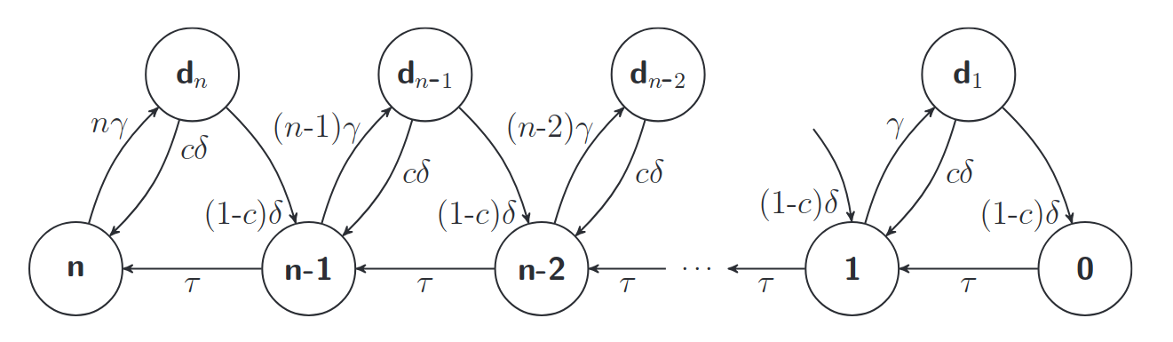
This Markov chain is irreducible, and we compute, fixed the interval , the average time the system spends in detected mode from time to time .
Denoting with the set of detected states, labeled as for in Figure 3, this measure, rephrasing what already seen in Section 3.5, can be computed as
In our test, we consider the interval of time , i.e., . The parameters are chosen as follows
In order to assess the scalability of our approach when the number of states grows, we consider large values of (even though those may not be common for the particular situation of a telecommunication system). The number of states in the Markov chain can be shown to be . The computational time required to compute the two measures is reported in Figure 5 for different values of ranging between and . We compare the timings with the cumulative solver included in Möbius 2.5 [10] that implement the uniformization method.
Instantaneous availability
| Möbius | exp_phi | |
|---|---|---|
The timings shows that, in this case, the computational complexity on the solver bundled with Möbius seems to have a quadratic complexity in the number of states. This appears to be caused by an increasing number of iteration needed to reach convergence due to relevant differences among rates in the Markov chain, which causes stiffness in the underlying ODE. The Krylov approach, on the other hand, does not suffer this drawback.
6.3 Reliability model for communication system attacks
We consider the mobile cyber-physical system model presented in [20], describing a collection of communicating nodes which are subject to attacks. The original study is based on a real-world architecture: there are mobile nodes, each node using sensors for localization and measuring anomaly phenomena, and the system comprises an imperfect intrusion/detection functionality distributed to all nodes for dealing with both intrusion and fault tolerance. This mechanism is based on a voting system. Here a simplified version is discussed, we refer the reader to [20] for further details on the intrusion/detection functionality and the complete system description.
The model considers a node capture which involves taking control of a good node by deceiving the authentication and turning it into a bad node that will be able to generate attacks within the system. The attackers primary objective is to cause impairment failure by performing persistent, random, or insidious attacks. At each instant of time, the number of good and bad nodes are indicated as and , respectively, and is the number of evicted nodes, i.e., nodes that have been detected as bad ones by the intrusion/detection mechanism. At the beginning, all nodes are considered good, i.e., . Only bad nodes can perform internal attacks, and whenever one of this attacks have success the entire system fails, switching the value of from , ok, to , failed.
The model is expressed through the definition of the Stochastic Reward Net depicted in Figure 6, where places (circles) correspond to , and determine the state of the system, and transitions (rectangles) define the behaviour of the attach model
- 1.
transition of a node from good to bad, called , represents the capture of a node by an attacker. The capture of a single node take place with rate , thus, being the capture of a node independent from the capture of other nodes, the rate of transition is .
- 2.
transition of a node from bad to evicted, called , represents the correct detection of an attack. Calling the probability of intrusion/detection false negative, and the period at which the intrusion/detection mechanism is exercised, the rate of is .
- 3.
transition of a node from good to evicted, called , represent a false positive of the intrusion/detection mechanism. Calling the probability of intrusion/detection false positive, the rate of is .
- 4.
transition of a the entire system from ok to failed, called . When a node is captured it will perform attacks with a probability and the success of attacks from compromised nodes has rate , thus the rate of is . At completion of transition the entire system fails and then both and are set to so that the Stochastic Reward Net reach a (failed) absorbing state.
The graph whose vertexes are all the feasible combinations of values within places and arcs correspond to transitions forms the Markov chain under analysis. For instance, with The Stochastic Reward Net of Figure 6 produces the Markov chain depicted in Figure 7, where the notation means and . The nonzero structure of the infinitesimal generator is reported in Figure 8.
The parameters are chosen as follows
Being the intrusion/detection mechanism based on a voting system, the Byzantine fault model is selected to define the security failure of the system, i.e., the situation in which the system is working but there are not enough good nodes to obtain consensus when voting, that in our system means . Thus, the cumulative measure of interest is
Instantaneous availability
| Möbius | exp_phi | |
|---|---|---|
We have tested our implementation and measured the time required to compute this measure. The results are reported in Figure 9. Beside some overhead when dealing with small dimensions (and times below seconds), the approach relying on the restarted Krylov method (labeled by exp_phi) is faster than the uniformization method included in Möbius.
6.4 Sensitivity analysis
As a last example, we consider the case of a sensitivity analysis. For simplicity, we consider once more the model of Section 6.1, and we assume to be interested in changing the parameter . The only ingredient missing is computing the derivative of with respect to , which in this case is simply given by the matrix
We have implemented the function computing the derivative of the measure following the approach described in Section 5, and the performance of the algorithm is reported in Figure 10, for the time . We see that also in this case the scalability of the asymptotic cost of the algorithm is linear with respect to the number of states, as expected.
| Time (s) | |
|---|---|
As demonstrated by the experiments, the Krylov based approach often outperforms the classical uniformization method. This could be explained by the fact that the Krylov method performs the number of restarts required to achieve a certain accuracy given a specific choice of and ; in the case of the uniformization, instead, one has to choose a small timestep when dealing with stiff problems, ignoring the effect of the left and right vectors and .
7 Conclusions
We have presented a novel point of view on the formulation of availability, reliability, and performability measures in the setting of Markov chains. The main contribution of this work is to provide a systematic way to rephrase these measures in terms of bilinear forms defined by appropriate matrix functions.
A dictionary translating the most common measures in the field of Markov modeling to the one of matrix functions has been described. We have proved that, leveraging the software available for the efficient computation of the action of on a vector, we can easily devise a machinery that evaluates these measures with the same or better performances that states of the art solvers, such as the one included in Möbius (which implements the uniformization method).
In particular, our solver seems to be more robust to unbalanced rates in the matrix and stiffness in general, which can make a dramatic difference in some cases, as showcased by our numerical experiments.
The new formulation allows to study measures’ sensitivity by a new perspective, namely Frechét derivatives. This appears to be a promising reformulation that, along with providing efficient numerical procedures, might give interesting theoretical insights in the future.
We expect that this new setting will allow to devise efficient method tailored to the specific structure of Markov chains arising, for instance, from different high-level modeling languages.
Several problems remain open for further study. For instance, we have analyzed the use of Krylov methods with restarts, but the use of rational Krylov methods appear promising as well. Moreover, often the infinitesimal generator have particular structures induced by the high-level formalism used to model the Markov chain — as it has often been noticed in the literature — which we have not exploited here. These topics will be subject to future investigations.
Appendix Appendix A Continuous time Markov chains and reward structures
Markov models are typically defined using high level formalism and then translated into CTMC. Most often, the modeler is interested in extracting relevant information on the Markov chain, such as probability of breakdown (or, from the opposite perspective, of completing operations without breakdown). This kind of information is described abstractly using a reward structure, which is defined at the higher level — using the MRP language. These measures assess the performance and dependability of the system, and so are called performability measures [23].
A.1 Definition of models and measures
Given a CTMC, a natural question is if the limit for of the probability distribution exists, and whether it depends on the initial choice . To characterize this behavior, we need to introduce the concepts of irreducibility.
Definition A.1.
Let be a Markov chain with infinitesimal generator , and consider the directed graph with nodes the set of states of , and with an edge from to if and only if . We say that is irreducible if for for every two states there exists a path connecting to . We say that is reducible if it is not irreducible.
We shall partition the Markov processes in two classes: the irreducible ones, called transient, which in the finite case are also positive recurrent, and the reducible ones, which are called terminating.
Intuitively, a Markov chain is irreducible if there is always a nonzero probability of jumping from to , possibly through some intermediate jumps. This property is sufficient to guarantee the existence and uniqueness of the steady-state vector , the limit of for .
From the linear algebra point of view, it is often useful to notice that a Markov process is reducible if and only if the matrix can be made block upper triangular by permuting the rows and column (with the same permutation).
We refer to the book [29] for a more detailed analysis on the classification of Markov chains, which we do not discuss further.
Theorem A.2.
Let be an irreducible Markov chain with a finite number of states and infinitesimal generator . Then, there exists a unique positive vector such that , and does not depend on . Moreover, generates the left kernel of .
A.2 Spectral properties of and the steady-state
As we already pointed out, unless the Markov chain is irreducible, the steady state probability might not be unique — and therefore depend on the specific choice of initial configuration . The uniqueness can be characterized by considering the spectral properties of .
Lemma A.3.
Let be the infinitesimal generator of a continuous time Markov chain. Then, is singular, and has as right eigenvector corresponding to the eigenvalue ; if the Markov process is irreducible, then the left kernel is generated by , the steady-state distribution.
The matrix has another distinctive feature from the linear algebra point of view, which we will use repeatedly in what follows.
Lemma A.4.
Let be the infinitesimal generator of a Markov chain. Then, is an -matrix, i.e., there exists a positive such that
with being a non-negative matrix with spectral radius bounded by .
Lemma A.4 implies, by a straightforward application of classical Gerschgorin theorems [30], that all the eigenvalues of are contained in the left half of the complex plane.
The spectral features of are tightly connected with the asymptotic behavior of the Markov chain. In particular, as we have pointed out in the previous section, a reducible process has a matrix that can be permuted to be block upper triangular. More precisely, one can reorder the entries as
| (1) |
where is a permutation that lists the indices in first, and then the ones in . The set are the transient states of the process, whereas contains the recurrent ones. The matrix contains the probability rates of jumping from a state in to a state in . The following characterization will be relevant in the following.
Lemma A.5.
Let be the infinitesimal generator of a terminating process, and the permutation identified in (1). Then, is invertible.
Proof.
We claim that every row of has the sum of the off-diagonal elements strictly smaller than the modulus of the diagonal one. We assume that the matrix has been permuted already, so we may write without loss of generality:
We have that, for every :
Considering that the diagonal element has negative sign, and all the others are positive, we conclude that
and therefore is not included in any of the Gerschgorin circles of , and is invertible [30]. ∎
A.3 Available solution methods
Solving the Markov chain means computing the probability vector at a given time or, if the chain is irreducible, computing the steady-state probability vector . As discussed in the following, often it is required to compute also for some index . We recall in this section the most well-known methods to tackle this task in the generic case (without particular assumption on the Markov chain).
A simple approach is the direct computation of the matrix exponential , which in turns allows to obtain . However, this is only feasible if the number of states is small, because the complexity is cubic in the number of states.
Another strategy is to compute the Laplace transform [29] of , denoted by , solving the linear system , obtained applying the Laplace transform to the Kolmogorov forward equation, and then anti-transform producing . The parameter can be chosen so that is non-singular, the linear system can be solved exploiting favorable properties of , e.g., sparseness, and the known term is often easy to compute because in dependability and performance models is highly structured. This method can be applied only to relatively small chains, being the anti-transform a costly operation, but can tackle relatively large . Numerical integration [27] from zero to of the Kolmogorov forward equation and/or of
where , is another alternative. Unfortunately, in dependability models the parameters can have different order of magnitudes, e.g., in a cyber-physical system the mean time to failure of an hardware component is considerably different from the mean time to failure of a software component, and similarly in performability models the performance-oriented and fault-related parameters can have different scalings. Thus, numerical integration is a good choice only if the chosen method, for the particular case under analysis, has been proved to be highly resilient to stiffness. For general chains and arbitrary , the uniformization method [27] is commonly adopted by commercial level software tool, such as Möbius [10]. An heuristically chosen such that allows to compute the truncate series expansion of and in terms of powers of . In the numerical experiments, we will compare the performances of the approach proposed in this paper with the solver bundled with Möbius.
A.4 Matrix functions
Matrix functions are ubiquitous in applied mathematics, and appear in diverse applications. We refer the reader to [17] and the references therein for more detailed information. The definition of a matrix function can be given in different (equivalent) ways. Here we recall the one based on the Jordan form.
Definition A.6 (Matrix function).
Let be a matrix with spectrum , and a function that is analytic on the spectrum of . Let be the Jordan form of , with being its decomposition in elementary Jordan blocks; we define the matrix function as
where for an Jordan block we have:
Definition A.6 is rarely useful (directly) from the computational point of view. In most cases, computation of matrix functions is performed relying on the Schur form, on block diagonalization procedures, on contour integration, or on rational and polynomial approximation (we refer to [17] and the references therein for a comprehensive analysis of advantages and disadvantages of the different approaches).
Remark A.7.
Note that, in order to apply Definition A.6, we do not necessarily need to be analytic on the whole spectrum of ; we just need to have derivatives of order at every point corresponding to an eigenvalue with Jordan blocks of size at most .
Some examples of matrix functions that appear frequently in applied mathematics are the matrix exponential , the inverse and the resolvents , the square root and the matrix logarithm .
Appendix Appendix B Rephrasing the measures
This section aims to provide the building blocks that enables the translation of the measures from the Markov chain setting, where they are expressed as expected values of a random variable obtained as a function of , to the more computationally-friendly matrix function form.
Proof of Lemma 2.3.
Recall that, by Definition 2.1, we have
by linearity of the integral. Assume, for simplicity, that is diagonalizable, and let be its eigendecomposition; we can write
By direct integration we get . Finally, using the relation we obtain the sought equality . The general statement follows by density of diagonalizable matrices, together with the continuity of . ∎
Remark B.1.
We shall note that defined in Lemma 2.3, despite being defined piece-wise, is an analytic function, and is in fact defined by the power-series
which is convergent for all . Nevertheless, the formula cannot be used directly to evaluate the function at , because is not well-defined when , and this point is always included in the spectrum, since is singular. The notation is often used in the description of exponential integrators. We refer to [16] and the references therein for more details.
A similar statement can be given also for the steady-state case. Nevertheless, to achieve this we need to consider a discontinuous function, and this can cause difficulties in the numerical use of such characterization.
Lemma B.2.
Let a continuous irreducible Markov process with infinitesimal generator , and assume an initial distribution of probability . The steady-state distribution can be expressed as follows:
Proof.
We notice that, for any finite time , . Since the spectrum of is contained in , it is sufficient to check that converges to as on this set. It is clear that, for every in the left half plane, we indeed have , and the claim follows noting that independently of . ∎
Remark B.3.
Remark B.4.
If the process is irreducible then the matrix function takes the form and therefore, since for every probability distribution , it is clear that the steady-state is independent of .
References
- [1] Afanasjew, M., Eiermann, M., Ernst, O. G., Güttel, S., 2008. Implementation of a restarted Krylov subspace method for the evaluation of matrix functions. Linear Algebra Appl. 429 (10), 2293–2314.
- [2] Al-Mohy, A. H., Higham, N. J., 2011. Computing the action of the matrix exponential, with an application to exponential integrators. SIAM J. Sci. Comput. 33 (2), 488–511.
- [3] Avizienis, A., Laprie, J.-C., Randell, B., Landwehr, C., Jan. 2004. Basic concepts and taxonomy of dependable and secure computing. IEEE Trans. Dependable Secur. Comput. 1 (1), 11–33.
- [4] Balsamo, S., Onvural, R. O., Persone, V. D. N., 2001. Analysis of Queueing Networks with Blocking. Kluwer Academic Publishers, Norwell, MA, USA.
- [5] Barbaresco, F., 2009. New foundation of radar doppler signal processing based on advanced differential geometry of symmetric spaces: Doppler matrix cfar and radar application. In: International Radar Conference. Vol. 82.
- [6] Benzi, M., Boito, P., 2014. Decay properties for functions of matrices over -algebras. Linear Algebra Appl. 456, 174–198.
- [7] Bini, D. A., Massei, S., Robol, L., 2017a. Efficient cyclic reduction for quasi-birth-death problems with rank structured blocks. Appl. Numer. Math. 116, 37–46.
- [8] Bini, D. A., Massei, S., Robol, L., 2017b. On the decay of the off-diagonal singular values in cyclic reduction. Linear Algebra Appl. 519, 27–53.
- [9] Crouzeix, M., Palencia, C., 2017. The numerical range is a -spectral set. SIAM J. Matrix Anal. Appl. 38 (2), 649–655.
- [10] Deavours, D. D., Clark, G., Courtney, T., Daly, D., Derisavi, S., Doyle, J. M., Sanders, W. H., Webster, P. G., 2002. The Möbius framework and its implementation. IEEE Trans. on Softw. Eng. 28 (10), 956–969.
- [11] Demmel, J. W., 1997. Applied numerical linear algebra. Vol. 56. Siam.
- [12] Estrada, E., Higham, D. J., 2010. Network properties revealed through matrix functions. SIAM Rev. 52 (4), 696–714.
- [13] Fenu, C., Martin, D., Reichel, L., Rodriguez, G., 2013. Network analysis via partial spectral factorization and Gauss quadrature. SIAM J. Sci. Comput. 35 (4), A2046–A2068.
- [14] Fletcher, P. T., Joshi, S., 2007. Riemannian geometry for the statistical analysis of diffusion tensor data. Signal Process. 87 (2), 250–262.
- [15] Frommer, A., Güttel, S., Schweitzer, M., 2014. Efficient and stable Arnoldi restarts for matrix functions based on quadrature. SIAM J. Matrix Anal. Appl. 35 (2), 661–683.
- [16] Gander, M. J., Güttel, S., 2013. PARAEXP: a parallel integrator for linear initial-value problems. SIAM J. Sci. Comput. 35 (2), C123–C142.
- [17] Higham, N. J., 2008. Functions of matrices. Theory and computation. Society for Industrial and Applied Mathematics (SIAM), Philadelphia, PA.
- [18] Hillston, J., 1996. A Compositional Approach to Performance Modelling. Cambridge University Press, New York, NY, USA.
- [19] Hochbruck, M., Lubich, C., Selhofer, H., 1998. Exponential integrators for large systems of differential equations. SIAM J. Sci. Comput. 19 (5), 1552–1574.
- [20] Martinez, J., Trivedi, K., Cheng, B., 2017. Efficient computation of the mean time to security failure in cyber physical systems. In: Proceedings of the 10th EAI International Conference on Performance Evaluation Methodologies and Tools. ICST, ICST, Brussels, Belgium, pp. 109–115.
- [21] Massei, S., Robol, L., 2017. Decay bounds for the numerical quasiseparable preservation in matrix functions. Linear Algebra Appl. 516, 212–242.
- [22] Meyer, J. F., 1980. On evaluating the performability of degradable computing systems. IEEE Transactions on computers (8), 720–731.
- [23] Meyer, J. F., July 1982. Closed-Form Solutions of Performability. IEEE Transactions on Computers C-31 (7), 648–657.
- [24] Plemmons, R. J., 1977. M-matrix characterizations. i—nonsingular m-matrices. Linear Algebra and its Applications 18 (2), 175–188.
- [25] Rathi, Y., Tannenbaum, A., Michailovich, O., 2007. Segmenting images on the tensor manifold. In: IEEE Conference on Computer Vision and Pattern Recognition. IEEE, pp. 1–8.
- [26] Reibman, A., Smith, R., Trivedi, K., 1989. Markov and Markov reward model transient analysis: An overview of numerical approaches. European Journal of Operational Research 40 (2), 257 – 267.
- [27] Reibman, A., Trivedi, K., 1989. Transient analysis of cumulative measures of Markov model behavior. Communications in Statistics. Stochastic Models 5 (4), 683–710.
- [28] Trivedi, K. S., 2002. Probability and Statistics with Reliability, Queuing and Computer Science Applications, 2nd Edition. John Wiley and Sons Ltd., Chichester, UK.
- [29] Trivedi, K. S., Bobbio, A., 2017. Reliability and Availability Engineering: Modeling, Analysis, and Applications. Cambridge University Press.
- [30] Varga, R. S., 2010. Geršgorin and his circles. Vol. 36. Springer Science & Business Media.
- [31] Yang, Q., Turner, I., Liu, F., Ilić, M., 2011. Novel numerical methods for solving the time-space fractional diffusion equation in two dimensions. SIAM J. Sci. Comp. 33 (3), 1159–1180.
- [32] Zhifeng, D., Fenghua, W., 2018. A generalized approach to sparse and stable portfolio optimization problem. Journal of Industrial & Management Optimization 14 (1547-5816_2018_4_1651), 1651.