Extreme Events: Mechanisms and Prediction
Abstract
Extreme events, such as rogue waves, earthquakes and stock market crashes, occur spontaneously in many dynamical systems. Because of their usually adverse consequences, quantification, prediction and mitigation of extreme events are highly desirable. Here, we review several aspects of extreme events in phenomena described by high-dimensional, chaotic dynamical systems. We specially focus on two pressing aspects of the problem: (i) Mechanisms underlying the formation of extreme events and (ii) Real-time prediction of extreme events. For each aspect, we explore methods relying on models, data or both. We discuss the strengths and limitations of each approach as well as possible future research directions.
1 Introduction
Extreme events are observed in a variety of natural and engineering systems. Examples include oceanic rogue waves [1, 2], extreme weather patterns [3, 4, 5, 6], earthquakes [7] and shocks in power grids [8, 9]. These events are associated with abrupt changes in the state of the system and often cause unfortunate humanitarian, environmental and financial impacts. As such, the prediction and mitigation of extreme events are highly desired.
There are several outstanding challenges in dealing with extreme events. These events often arise spontaneously with little to no apparent early warning signs. This renders their early prediction from direct observations a particularly difficult task [10, 11, 12]. In certain problems, such as earthquakes, reliable mathematical models capable of predicting the extreme events are not available yet [13].
In other areas, such as weather prediction where more advanced models are in hand, accurate predictions require detailed knowledge of the present state of the system which is usually unavailable. The partial knowledge of the current state together with the chaotic nature of the system leads to uncertainty in the future predictions. These uncertainties are particularly significant during the extreme episodes [14, 15, 16].
In addition, models of complex systems are usually tuned using data assimilation techniques. This involves selecting the model parameters so that its predictions match the existing empirical data. The effectiveness of data assimilation, however, is limited when it comes to rare extreme events due to the scarcity of observation data corresponding to these events [17, 18, 19, 20].
These challenges to modeling and prediction of extreme events remain largely outstanding. The purpose of the present article is to review some of these challenges and to present the recent developments toward their resolution.
The analysis of extreme events can be divided into four components as illustrated in figure 1: Mechanisms, Prediction, Mitigation and Statistics. Below, we briefly discuss each of these components.
- (i)
Mechanisms: The mechanisms that trigger the extreme events are the primary focus of this article. Consider an evolving system that is known from the time series of its observables to produce extreme events. We are interested in understanding the conditions that underly the extreme events and trigger their formation. Even when the governing equations of the system are known, it is often a difficult task to deduce the mechanism underlying the extreme events. This is due to the well-known fact that even seemingly simple governing equations can generate very complex chaotic dynamics. The task of deducing the behavior of solutions from the governing equations becomes specially daunting when the system consists of many interacting degrees of freedom which give rise to a high-dimensional and complex attractor.
In section 3, we review a number of methods that unravel the extreme event mechanisms. These methods have been developed to analyze specific classes of dynamical systems. For instance, the multiscale method discussed in section 3.1 only applies to systems whose degrees of freedom can be separated into the so-called slow and fast variables. Even when such a slow-fast decomposition is available, computing the corresponding slow manifold and its stable and unstable manifolds become quickly prohibitive as the dimension of the system increases.
As a result, a more general mathematical framework is needed that is applicable to a broader range of dynamical systems and at the same time can leverage the ever growing computational resources. We explore such a general framework in section 4.
- (ii)
Real-time prediction: Most undesirable aspects of extreme events can often be avoided if the events are predicted in advance. For instance, if we can predict severe earthquakes a few hours in advance, many lives will be saved by evacuation of endangered zones. As a result, their real-time prediction is perhaps the most exigent aspect of extreme phenomena.
Real-time prediction requires measurable observables that contain early warning signs of upcoming extreme events. We refer to such observable as indicators of extreme events. Reliable indicators of extreme events must have low rates of false-positive and false-negative predictions. A false positive refers to the case where the indicator incorrectly predicts an upcoming extreme event. Conversely, a false negative refers to the case where the indicator fails to predict an actual extreme event. Knowing the mechanisms that trigger the extreme events does not necessarily enable their prediction. However, as we show in section 5, even partial knowledge of these mechanisms may lead to the discovery of reliable indicators of extreme events.
Another important aspect of extreme event prediction is the confidence in the predictions. The sensitivity to initial conditions leads to an inherent uncertainty in chaotic systems even when the system model is deterministic [21, 22]. Such uncertainties permeate the prediction of extreme events. As a result, the predictions have to be made in a probabilistic sense where the uncertainties in the predictions are properly quantified (see section 5.1).
- (iii)
Mitigation: Can we control a system so as to suppress the formation of extreme events? This if of course beyond reach in many natural systems such as ocean waves and extreme weather patterns. However, in certain engineered systems, such as power grids, one can in principle design control strategies to avoid the formation of extreme events [23, 24, 25]. To this end, knowing the mechanisms that trigger the extreme events is crucial as it informs the design of the control strategy. The real-time prediction of the extreme events, on the other hand, informs the optimal time for the activation of the control strategy (see figure 1).
The mitigation of extreme events within a dynamical systems framework has only recently been examined [26, 27, 28, 29, 30, 31]. The research in this direction has been limited to mitigation in simplified models by introducing arbitrary perturbations that nudge the system away from the extreme events. However, a systematic study involving controllability and observability of extreme events in the sense of control theory is missing.
- (iv)
Statistics: The statistical study of extreme events attempts to answer questions regarding the frequency and probability of occurrence of extreme events from a large sample. Such statistical questions are perhaps the most intensely studied aspect of extreme events due to their applications in finance, insurance industry and risk management [32, 33, 34, 35]. In this article, we will limit our discuss of the statistics to this section and refer the interested reader to the cited literature on the topic.
Two major frameworks for quantifying the extreme statistics of stochastic processes are the extreme value theory and the large deviation theory. The extreme value theory studies the probability distribution of the random variable where is a sequence of random variables [36]. The main objective in extreme value theory is to determine the possible limiting distributions of as tends to infinity. In particular, the Fisher–Tippett–Gnedenko theorem (also known as the extremal types theorem) states that, if is a sequence of independent and identically distributed (i.i.d) random variables then the limiting distribution of can only converge to three possible distributions and provides explicit formula for these distributions [37, 38, 39]. This is a significant result since the extreme statistics of the random variable can be deduced even when no extreme events have actually been observed. In many practical cases, however, the random variables are not independent. Therefore, the more recent work in extreme value theory has been focused on relaxing the independence assumption [40, 41, 42, 43, 44, 45, 46, 47, 48]. For an extensive review of extreme value theory in the context of dynamical systems, we refer to a recent book by Lucarini et al. [49].
Another prominent framework for the statistical analysis of extreme events is the large deviation theory which is concerned with the tail distribution of random variables. The tails of the probability distributions contain the extreme values a random variable can take, hence the name large deviations. The large deviations were first analyzed by Cramèr [50] who studied the decay of the tail distribution of the empirical means for where is a sequence of i.i.d random variables. Later, Donsker and Varadhan [51, 52, 53, 54] generalized the large deviation results to apply them to Markov processes. The current scope of the large deviation theory is quite broad and is applied to quantifying heavy tailed statistics in a variety of deterministic and stochastic dynamical systems. We refer the interested reader to the articles by Varadhan [55] and Touchette [56, 57] for a historical review of large deviation theory and its applications.
The four aspects of extreme events mentioned above are intertwined. However, the discovery of mechanisms that give rise to extreme events resides in the heart of the problem (see figure 1). For instance, even partial knowledge of the mechanisms that trigger the extreme events may lead to the discovery of indicators that facilitate their data-driven prediction (see section 5.2). In addition, once we know what mechanisms trigger the extreme events, we can make informed choices about the control strategies towards avoiding them. To this end, the real-time prediction of upcoming extreme events informs the time the control strategy should be activated. Knowledge of the mechanisms of the extreme events can also help improve the statistical estimates regarding their likelihood and frequency.
As a result, the main focus of this article will be on the first aspect of extreme events, i.e., the mechanisms. We will also discuss some aspect of the real-time prediction of the extremes, specially the quantification of the reliability of the indicators of extreme events. In section 2, we introduce the general set-up and notation. Section 3 reviews some well-known mechanisms for extreme event formation in deterministic and stochastic dynamical systems. In section 4, we review a variational method for discovering the mechanisms of extreme events and illustrate its application with two examples: intermittent turbulent energy dissipation and rogue ocean waves. In section 5, we discuss reliable indicators of extreme events for their real-time prediction. Section 6 contains our concluding remarks.
2 Setup and notation
In this section, we lay out the setup of the problem that allows for a dynamical systems framework for extreme event analysis. We consider systems that are governed by an initial value problem of the form
| (1a) | |||
| (1b) |
where the state belongs to an appropriate function space for all times . The initial state of the system is specified by , where and . The operator is a potentially nonlinear operator that is provided by the physics. The PDE (1) should also be supplied with appropriate boundary conditions where denotes the boundary of .
System (1) generates a solution map
| (2) |
that maps the initial state to its image at a later time . The solution map has the semi-group property, i.e., and for all .
We equip the space with further structure. In particular, we assume that is a probability space and that the probability measure is -invariant. We refer to a measurable function as an observable. Note that for an observable , is a continuous stochastic process whose realizations are made by choosing an initial condition drawn in a fashion compatible with the probability measure .
The observable is a quantity whose statistics and dynamical evolution is of interest. For instance, in the water wave problem considered in section 4.3 below, the observable is the wave height. In meteorology, the observable of interest could be temperature or precipitation. Here, we are in particular interested in the extreme values of the observable . In practice, the extreme values are often defined by setting a threshold . The observable values that are larger than this threshold constitute an extreme event. This motivates the following definition of extreme events.
Definition 1 (Extreme Events)
For an observable , the extreme event set , corresponding to the prescribed extreme event threshold , is given by
| (3) |
The extreme event sets within the state space are depicted in figure 2. As the system trajectory passes through the extreme event set , the time series of the observable exhibit a sudden burst. In this figure, the extreme event set is depicted as a collection of patches, but in principle this set can have an extremely complex geometry.
In certain problems, the extreme events may correspond to unusually small values of the observable . In that case, Definition 1 is still operative by studying the observable instead of . A third type of rare events (which are not necessarily extreme) is the rare transition between long-lived states (see figure 3). In this case, the system evolves for long times around a particular state before it is suddenly ejected to the neighborhood of a different state around which the system evolves for a long time before being ejected again [58, 59, 60, 61, 62, 63, 64]. Although such rare transitions do not necessarily fall under Definition 1, we return to them in section 3.3 and review the mechanisms that cause the transitions.
Finally, we point out that, although the governing equations (1) are formulated as a partial differential equation (PDE), we will also consider systems that are described by a set of ordinary differential equations (ODEs), , where denotes the state of the system at time . This ODE could also arise from a finite-dimensional approximation of a PDE model as is common in numerical discretization of PDEs.
3 Routes to extreme events
There are certain classes of dynamical systems exhibiting extreme events for which the mechanisms that trigger these events are well-understood. In this section, we review three such systems and discuss the underlying mechanisms of extreme events in them.
3.1 Multiscale systems
An interesting type of extreme events appear in slow-fast dynamical systems where the motion is separated into distinct timescales. The extreme events in such systems appear as bursts when a system trajectory is dominated by the fast timescales of the system. The early work on this subject was motivated by the observation of relaxation oscillations in electrical circuits [65, 66, 67]. Later, slow-fast dynamics found applications in a wide range of problems such as chemical reactions [68, 69, 70, 71, 72], excitable systems (e.g., neural networks) [73, 74, 75, 76, 77, 78, 79], extreme weather patterns [80, 81, 82], and dynamics of finite-size particles in fluid flows [83, 84].
We first discuss the phenomenology of bursting in slow-fast systems and then demonstrate its implications on a concrete example. Figure 4 sketches the phase space geometry of a slow-fast system. It has an invariant slow manifold where the trajectories follow the slow time scale. In the directions transverse to the slow manifold, the dynamics follow the fast time scales. We assume that the slow manifold is normally hyperbolic. Loosely speaking, normal hyperbolicity means that the transverse attraction to and repulsion from the manifold is stronger than its internal dynamics [85, 86]. We also assume that the slow manifold is of the saddle type, that is, it consists of two components: attracting and repelling. Normal perturbations to the manifold on its attracting component decay over time while the perturbations over the repelling component grow. Due to invariance of the slow manifold, trajectories starting on the manifold remain on it for all times unless they exit the manifold through its boundaries.
Now consider a trajectory that starts slightly off the slow manifold over its attracting component (the black curve in figure 4). Initially this trajectory converges towards the slow manifold until it approaches its repelling component. At this point, the normal repulsion pushes the trajectory away from the slow manifold where the fast time scales are manifest. This rapid repulsion continues until the trajectory leaves the neighborhood of the repelling component and is pulled back towards the attracting components.
If the normal repulsion is strong enough, the episodes where the trajectory travels away from the slow manifold appear as rapid bursts. The repelling subset of the slow manifold can be a very complex set as a result of which the burst can appear chaotic and sporadic.
We demonstrate the bursting in slow-fast systems on a normal form of a singular Hopf bifurcation [87],
| (4) |
where is a small parameter. For our discussion we fix the remaining parameters, , , and .
We first discuss the singular limit where . In this limit, system (4) reduces to the differential-algebraic equations
| (5) |
This reduced system describes the slow flow on the critical manifold
| (6) |
In order to discern the dynamics outside the critical manifold, we use a blow-up construction by rescaling time according to . The derivative with respect to the fast time is given by . With this change of variable, equation (4) becomes
| (7) |
where the prime denotes derivative with respect to the fast time . In the singular limit, , we have and . Moreover, in the rescaled system, every point on the critical manifold is a fixed point since . This is an artifact of the rescaling which is singular at . More precisely, points on the critical manifolds are fixed points with respect to the fast time scale. In turn, the slow dynamics on the critical manifold is given by the reduced system (5). The combination of the reduced system (5) and the rescaled system (7) describes the motion on the critical manifold and away from it.

Of particular relevance to us is the behavior of trajectories in a small neighborhood of the critical manifold. The critical manifold consists of three connected components (see figures 5 and 6). Two of these components, denoted by , are normally attracting, meaning that trajectories starting away from them in a transverse direction converge towards the critical manifold. In contrast, transverse perturbations to the normally repelling segment diverge rapidly from the critical manifold. As a result, trajectories starting near the repelling submanifold are repelled to a neighborhood of the attracting manifold where they follow the slow time scales along the critical manifold until they reach one of the fold points or (see figure 5). At the folds, located on the boundary between the attracting and repelling submanifolds, the trajectory is repelled again from toward the second segment of the attracting submanifold . This cycle continues indefinitely, creating bursting trajectories that are repelled away from the repelling submanifold and attracted back towards the critical manifold along its attracting segment.
Now we turn our attention to the nonsingular case where . The above analysis of the singular flow () bears some relevance to the nonsingular case (). For sufficiently small perturbations, , the Geometric Singular Perturbation Theory (GSPT) [88] guarantees, under certain conditions, that the critical manifold survives as a perturbed invariant manifold , that is as smooth as the critical manifold, and that is close to the critical manifold . Furthermore, the normally attracting or repelling properties of the perturbed manifold is similar to that of the critical manifold .
In particular, for system (4), the critical manifold deforms into a nearby slow manifold . The perturbed slow manifold has its own repelling and attracting submanifolds similar to those of which create bursting repulsion from and attraction towards the slow manifold. Figure 6 shows a trajectory of the system for . At this parameter values, the system has undergone a supercritical Hopf bifurcation [89] giving birth to a stable periodic orbit (the black curve). This periodic orbit carries much of the bursting properties described above for the singular system. Most of the time, the trajectory spirals outwards near the fold . At some point, the trajectory approaches the repelling segment of the slow manifold whereby it is repelled away towards its attracting segment. The trajectory follows the attracting segment until it reaches the fold where the repelling segment again repels the trajectory towards the second attracting segment. Following the attracting segment, the trajectories returns towards the fold and the small spiral motion repeats. This cycle continues indefinitely. Figure 6(c) shows the time series of the -coordinate along the periodic orbit showing the bursts resulting from repulsion away from the slow manifold.
For illustrative purposes, we presented in figure 6 a parameter set where the asymptotic motion of the system is relatively simple, dictated by a single stable periodic orbit. The dynamics is not always so predictable. There are parameter values where the system undergoes period doubling bifurcations resulting in several co-existing unstable periodic orbits. As a result, a generic trajectory never settles down to a particular periodic orbit. Instead, it indefinitely bounces back and forth between unstable periodic orbits. As a result, the bursting time series appear chaotic and less predictable.
We illustrate this on a system which exhibits chaotic bursts for a wide range of parameters. Consider the coupled FitzHugh–Nagumo units [77],
| (8) |
where is the number of units and are constant parameters. The units are coupled to each other through the summation term. The matrix with entries is the adjacency matrix that determines which units are coupled. The constant determines the strength of the couplings.

Figure 7 shows a typical trajectory of the FitzHugh–Nagumo system with two units (). Also shown is the time series of the mean of , i.e. . The mean mostly oscillates chaotically around with a relatively small variance. Once in a while, however, it exhibits relatively large excursions away from in the form of bursts. As opposed to the periodic extreme events of figure 6, these bursts appear chaotically, with no regular recurrent pattern. Similar extreme events have been observed in the FitzHugh–Nagumo system with larger number of units and various parameter values [78].
In this chaotic regime, the geometry of the invariant sets and their stable and unstable manifolds can be incredibly complex. One of the recent contributions to the field of slow-fast systems has been the development of accurate numerical methods for computing such invariant manifolds [90, 91, 92, 93]. The computational cost of these manifolds increases with the dimension of the system such that their computation is currently limited to four or five dimensional systems [94]. Nonetheless, understanding the mechanism behind extreme events in prototypical low-dimensional slow-fast systems has been greatly informative at the conceptual level.
3.2 Homoclinic and heteroclinic bursting
Another geometric mechanism of generating extreme events is through homoclinic and heteroclinic connections (see figure 8). Since these mechanisms share many of the characteristics of the slow-fast systems discussed in section 3.1, we limit this section to a brief discussion of the main ideas underlying homoclinic and heteroclinic bursting.
An example of a homoclinic connection is that of the Shilnikov orbit of a saddle-focus fixed point. This is an unstable fixed point with a two-dimensional stable manifold and a one-dimensional unstable manifold (see figure 8(a)). Within the stable manifold, the trajectories spiral towards the fixed point while they are repelled from the fixed point in its unstable direction. The Shilnikov orbit is the homoclinic trajectory that is asymptotic to the fixed point both in forward time and in backward time.
Shilnikov [95] proved that, if the attraction within the stable manifold is weaker than the repulsion along the unstable manifold, small perturbations to the system give birth to infinitely many unstable periodic orbits around the homoclinic orbit. These periodic orbits resemble the shape of the original Shilnikov orbit [96]. More precisely, the periodic orbits consist partly of spiral motion towards the fixed point and partly of bursting motion away from it. Generic trajectories shadow these periodic orbits such that the time series of their -component exhibits small scale oscillations, corresponding to the spiraling motion, and occasional bursts, corresponding to repulsion along the unstable manifold [97, 98]. Since the periodic orbits are all unstable, the motion along generic trajectories can be chaotic resulting in very complex dynamics. A classical example of such chaotic motion is the Rossler attractor [99, 100].
Although the Shilnikov bifurcation was first studied as a route to chaotic motion in simple systems, it has found many applications in explaining the self-sustained bursting phenomena observed in nature. These include, for instance, sudden variations in geophysical flow patterns [101, 102], spiking and synchronization in neural networks [103, 75, 104] and chemical reactions [105].
A similar mechanism of bursting is through heteroclinic connections. As opposed to the homoclinic case, the heteroclinic orbit asymptotes to different fixed points in forward and backward times. Figure 8(b), for instance, depicts a heteroclinic connection corresponding to the phase space of a three-dimensional vector field introduced in Ref. [106]. As in the homoclinic case, the heteroclinic bursting has been useful in explaining several spiking behavior observed in nature from nonlinear waves to turbulent fluid flow [107, 108, 109, 110, 111, 112, 113].
3.3 Noise-induced transitions
So far we have discussed deterministic systems which possess a self-sustaining mechanism for generating extreme events. However, an important class of rare extreme events are induced by noise [114, 115, 116, 117]; see also [118] for an excellent review for this form of transitions. Such systems typically have equilibria that are stable in the absence of noise. Noise, however, makes it possible to transition from the neighborhood of one equilibrium to the other.
In such systems the transition mechanism is the noise and, as such, there is no ambiguity regarding what underlies the rare events. However, the route the system takes during each transition is not as clear. In fact, due to the random nature of the system, the transition routes can only be identified probabilistically. In particular, one can inquire about the most likely route the system takes in traveling between two states. The answer facilitates the prediction of individual transitions as well as the quantification of transition rates in an ensemble of experiments. In this section, we briefly review the transition-path theory which is a framework for addressing these questions.
The origins of the transition-path theory stem from chemical physics where one is interested in computing the rate of chemical reactions that lead to a transition from the reactant state to the product state [119, 120, 58, 121, 122, 123].
The transition-path theory aims to go beyond computing the transition rates and determines the most likely paths that the system may take during the transitions. To describe this theory, we consider the Langevin equation,
| (9) |
where determines the state of the system, is the mass matrix, is the potential and is the friction coefficient. The stochastic process is a white noise with mean zero and covariance and is the diffusion matrix.
For our introductory purposes it is helpful to consider the over-damped case where equation (9) reduces to
| (10) |
where determines the state of the system. For simplicity, we have assumed and rescaled time to eliminate the dependence on the friction coefficient .
Figure 3 sketches the over-damped system (10) in the one-dimensional case (). In absence of noise , the system converges asymptotically to one of the two local minima of the potential . The noise, however, nudges the trajectory away from these equilibria. In rare instances, the trajectory can even pass over the saddle separating the two equilibria causing a transition from equilibrium towards equilibrium and vice versa.
In this simple example, there is no ambiguity about the path these rare transitions take since there is only one degree of freedom available. However, in higher dimensional problems (), the rare transitions have more options for traveling between local minima of the potential . Figure 9(a), for instance, shows the so-called rugged Mueller potential in two dimensions () with infinitely many possible paths between any pair of local minima.
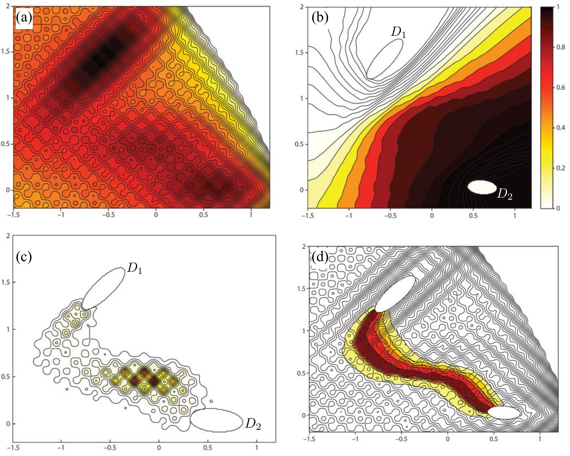
In this case, the following question arises: Given two sets , what is the most likely path the system may take for transitioning from set to set ? Figure 9(b) shows two such sets that cover the the lowest valleys of the potential . To answer this question, we assume that system (10) is ergodic with a unique invariant probability density such that the probability density of observing the state is . We would like to find the probability density which corresponds to the probability that a trajectory passing through has come from and will be going to . This probability density is given by
| (11) |
where are the so-called committor functions. The committor function measures the probability that a trajectory passing through came from . On the other hand, measures the probability that the trajectory passing through will arrive at before arriving at .
One can show that the committor functions satisfy the backward Kolmogorov equations
| (12) |
and
| (13) |
where is a linear operator and is its adjoint with respect to the inner product (see, e.g., Refs. [125, 62]). In addition, the density satisfies the forward Kolmogorov (or Fokker–Planck) equation,
| (14) |
where the time derivative vanishes since the density is invariant.
In order to evaluate the transition probability density , one needs to solve equations (12), (13) and (14) for , and , respectively. Then the transition probability density is computed from (11). Figure 9(c) shows the transition probability density corresponding to the rugged Mueller potential.
Recall that the probability density corresponds to the probability that a trajectory passing through has come from and will be going to . Although useful, this probability density is still a pointwise quantity which does not immediately inform us about the most likely path the system will take in going from to .
To address this shortcoming, the transition-path theory uses the probability current associated with the transition probability density . The vector field is defined such that for any codimension-one surface the integral of over the surface, i.e. , equals the probability flux of transition trajectory through . The current can be expressed explicitly in terms of the quantities introduced previously [125, 62] as
| (15) |
where is the probability current associated with the probability density .
Figure 9(d) shows the streamlines of the transition current . The color encodes the probability of the transition along each path such that the darker colors mark a higher transition probability. This figure finally shows the most probable path the transitions trajectories take in going from to .
Therefore, for noise-driven rare transitions, the transition-path theory provides a rigorous framework for computing the most likely mechanism for the rare events. We recall, however, that computing the transition paths in this framework requires the solutions to three PDEs (12), (13) and (14). Solving these equations in higher dimensions are quite costly such that the applications of transition-path theory have been limited to two- and three-dimensional systems [63]. We finally point out that a number of numerical methods for approximating the rare transition paths have been developed in order to partially remedy this high computational cost [126, 127, 128, 129, 130, 131, 132].
4 Variational method for physics-based probing of extreme events
In this section, we review a recent variational method for discovering the mechanisms that cause the extreme events. This method exploits the physics given by the governing equations (1) together with the statistical information from the system attractor in order to find initial states that over a prescribed time interval develop into an extreme event. The hope is to learn about the mechanism that causes the extremes by examining the states that precede the extreme events. We first introduce the variational method in a general framework and then present two specific applications of the method.
4.1 The variational method
Consider an observable whose time series along the system (1) is known to exhibit extreme events (see Definition 1). Also assume that there is a typical timescale over which the observable grows from its typical values and increases past its extreme value threshold . We therefore seek initial states such that . This motivates the definition of the domain of attraction of extreme events as follows.
Definition 2 (Extreme Event Domain of Attraction)
For an extreme event set and a prescribed time , the corresponding finite-time domain of attraction to the extreme events is the set
| (16) |
Here is shorthand for the pre-image of a set . The set contains the states that at some future time , with , enter the extreme event set . We remove the extreme event set from the domain of attraction to exclude the states that are extreme at the initial time.
The extreme event domain of attraction can be an extremely complex set whose numerical estimation is a daunting task. In addition, determination of the entire set may be unnecessary for deciphering the mechanisms that give rise to extreme events. Instead, one representative state from this set may suffice in discovering the extreme event generating mechanism.
We proposed in [133] to obtain the desired representative states as the solutions of a constrained optimization problem. In this approach, we seek states that maximize the growth of the observable over a prescribed time interval of length . More precisely, we seek the solutions to the maximization problem
| (17) |
where is a subset of to be discussed shortly. There are two constraints that are embedded in the optimization problem (17). One constraint is enforced through generated by the governing equations (1). In other words, it is implicitly implied that is a solution of the governing equations.
A second constraint is implied by requiring the state to belong to the subset . We envision to approximate the attractor of the system (1). This constraint is essential for discarding exotic states that belong to the state space but have negligible probability of being observed under the natural dynamics generated by the governing equations. It is known that dissipative differential equations often posses an attractor which is a subset of the state space [134, 135]. While the system can be initialized from any arbitrary states , its trajectories quickly converges to the attractor and remain on it. As a result, much of the function space is unexplored; the only states relevant to long term dynamics of the system are the ones belonging to the attractor or a small neighborhood of it. To this end, this additional constraint not only leads to more relevant states as precursors, but it also reduces the computational cost of the optimization problem, since we explore only the physically relevant solutions. For instance, the state space of the FitzHugh–Nagumo system shown in figure 7 is . However, it is visually appreciable that its trajectories converge to a small subset of .
Constraining the optimal states in equation (17) to belong to the attractor eliminates the states that may lead to a large growth of the observable but are dynamically irrelevant. The FitzHugh–Nagumo system, for instance, has transient trajectories along which becomes larger than which is much larger than the typical bursts shown in figure 7. These unusually large bursts, however, occur along trajectories that are away from the attractor and therefore are not sustained.
The attractor can be a very complex set whose estimation is quite difficult. In fact, numerical approximation of the attractors even in low-dimensional systems is an active area of research (see, e.g., Refs. [136, 137]). For our purposes an approximate representation of the attractor is sufficient. Here, we assume that the attractor can be approximated by the set
| (18) |
where determines the number of constraints, the maps are smooth enough and are the lower and upper bounds of . The choice of the maps and their bounds depends on the problem and is elaborated in the following sections.
With the two constraints discussed above, the optimization problem (17) can be written more explicitly as
| (19a) | |||
| (19b) | |||
| (19c) |
where is the shorthand notation for a trajectory of the system (1). If the set is compact in and the observable and the solution map are smooth enough, then there exist solutions to problem (19). These solutions are not necessarily unique. In fact, often there are multiple local maxima which may or may not be informative as to the origins of the extreme events. The relevance of the local minimizers can only be determined a posteriori. There are standard numerical methods for approximating the solutions of the constrained optimization problems of the form (19) that we do not review here but refer the interested reader to Refs. [138, 139, 140, 141].
Let denote a solution of the problem (19) corresponding to an extreme event, i.e., . We point out that a generic trajectory of the system (1) may never exactly pass through the state . However, if the solution map is continuous, any trajectory passing through a sufficiently small neighborhood of will also develop into an extreme event. This is illustrated in figure 10.
We demonstrate the application of this variational method on two examples. The first example involves the discovery of internal energy transfers that lead to the extreme energy dissipation episodes in a turbulent fluid flow. The second examples involves prediction of unusually large ocean surface waves, commonly known as rogue waves.
4.2 Application to a turbulent fluid flow
In this section, we present the application of the variational method to the extreme energy dissipation in a turbulent fluid flow. This flow is analyzed in detail in Ref. [133]; here, we reiterate our main findings and add a number of complementary comments. Consider the solutions to the two-dimensional incompressible Navier–Stokes equation
| (20) |
where is the velocity filed, is the pressure field, is the kinematic viscosity and the torus is the fluid domain with periodic boundary conditions. The velocity and pressure are functions of the spatial variables and time . The flow is driven by the deterministic Kolmogorov forcing where is the forcing wavenumber and . The simulations start from a random initial condition which is in turn propagated forward in time by numerically integrating the Navier–Stokes equation (20). We allow enough time elapse before collecting data in order to ensure that the initial transients have decayed and the trajectory has settled to the system attractor.


Because of the simplicity of the forcing and the boundary conditions, the Kolmogorov flow (i.e. the Navier–Stokes equations driven by the Kolmogorov forcing) has been studied extensively both by numerical and analytical methods [142, 143, 144, 145, 146, 113]. Similar variants of the Kolmogorov flow have also been investigated experimentally [147, 148, 149, 150].
In spite of the simplicity of the forcing and the boundary conditions, the Kolmogorov flow exhibits complex chaotic dynamics when the Reynolds number is sufficiently large. In particular, the Kolmogorov flow is known to undergo intermittent bursts in this chaotic regime [113]. The bursts are detected by monitoring certain system observables such as the energy dissipation rate and the energy input rate ,
| (21) |
The energy input rate measures the rate at which the external forcing pumps energy into the system. The energy dissipation rate measures the rate at which the system dissipates energy through diffusion.
Figure 11(a) shows the time series of the energy dissipation rate along a typical trajectory of the Kolmogorov flow at . This time series clearly exhibits chaotic, short-lived bursts. The bursts of the energy dissipation are almost concurrent with the bursts of the energy input rate . This can be inferred from figure 11(b) showing the joint probability density associated with the joint probability distribution
| (22) |
where is the invariant probability measure induced by the solution map of the Kolmogorov flow (cf. section 2). In practice, the density is approximated from data sampled from long-time simulations along several trajectories [151].
Since the large values of correlate strongly with the large values of (figure 11(b)), it is reasonable to assume that the same mechanism instigates the bursts of both quantities. From a physical point of view, one is interested in the burst of the energy dissipation rate . However, since the energy input rate is linear in the velocity field , it is mathematically more convenient to work with this quantity.
Given the simple form of the Kolmogorov forcing , the energy input rate (21) can be written more explicitly as where are the Fourier coefficients such that
| (23) |
where . This Fourier series is written in a divergence-free form so that the incompressibility condition is ensured. The energy input rate can be written in terms of the modulus and phase of the Fourier coefficients as where . Therefore, there are two scenarios through which the energy input rate can increase: (i) For a fixed , the phase approaches resulting in and subsequently increasing . (ii) For a fixed phase , the modulus increases resulting in the growth of .
Scenario (i) implies the alignment of the external forcing and the velocity field in the function space. This scenario, although appearing a priori more likely, is rejected based on numerical observations (see Ref. [133] for more details). Instead, it is the increase in the modulus that in turn leads to the increase in during its bursts (scenario (ii)). The growth of is only possible through the internal energy transfers operated by the nonlinear term . It is known that the nonlinear term redistributes the energy (injected by the external forcing) among the Fourier modes in such a way that the total transfer of energy among modes is zero [152, 153]. Note that both the nonlinear term and the pressure gradient conserve energy since
| (24) |

Examining the structure of the Navier–Stokes in the Fourier space reveals that Fourier modes are coupled together in triads such that the mode is affected by pairs of modes and with [152]. Each set of modes whose wavenumbers satisfy are referred to as a triad. Since each mode may belong to several triads [153], they form a complex network of triad interactions that continuously redistributes the energy among various modes. As a result, it is not straightforward to discern the mode(s) responsible for the growth of the modulus of the mode , resulting in the bursts of the energy input .
In Ref. [133], we employed a constrained optimization similar to (19) to discover the modal interactions that cause the extreme events in the Kolmogorov flow. Skipping the details, figure 12 shows the obtained optimal solution in the Fourier space. This optimal solution essentially consists of three Fourier modes with wavenumbers , and . Interestingly, these three modes form a triad since . Moreover, the wavenumber is present in this triad supporting scenario (ii) that postulated that the internal transfers of energy to mode are responsible for extreme events in the Kolmogorov flow.
Figure 13 shows the evolution of the moduli and along a typical trajectory of the Kolmogorov flow. First, we notice that has bursts similar to those of the energy dissipation rate (see figure 11). Secondly, the modulus has sharp dips which are almost concurrent with the bursts of . This observation shows that, during extreme events, the mode loses its energy and transfers most of it to mode through the triad interaction . The increase in , in turn, leads to an increase in the energy input rate causing the observed bursts in (see figure 11).
How does this transfer of energy from a low wavenumber to a higher wavenumber cause the bursts in the energy dissipation rate ? To answer this question we observe that
| (25) |
which follows directly from the definition of the energy dissipation (21) and the Fourier series (23). The transfer of energy from the mode to the mode will significantly increase the energy dissipation rate since the term is multiplied by a larger prefactor compared to the term whose prefactor is .
4.3 Application to oceanic rogue waves
In this section, we consider the real-time prediction of rogue water waves. Rogue waves refer to unusually large waves when compared to the surrounding waves. While there is no rigorous definition of a rogue wave, it is customary to define it as a wave whose height exceeds twice the significant wave height. For a given sea state, the significant wave height refers to four times the standard deviation of the surface elevation [1].
As a starting point, we consider the free-surface, as an unidirectional, irrotational flow in deep seas. The surface elevation is a function of the horizontal spatial variable and time (see figure 14). The vertical coordinates are denoted by the variable , such that the velocity potential is given by . In this setting, the water waves are governed by the set of equations [154],
| (26a) | |||
| (26b) | |||
| (26c) | |||
| (26d) |
Equation (26a) is the Bernoulli equation for irrotational flows with a free surface. Equation (26b) follows from the conservation of mass. Equations (26c) and (26d) are the boundary conditions at the bottom of the sea and the surface, respectively. The constant denotes the gravitational acceleration.
To solve the water wave equations (26) numerically, we need the initial surface elevation and the initial velocity potential . While the practical measurement of the surface elevation is possible [155, 156, 157, 158], measuring the entire velocity potential beneath the surface remains a challenging task. Therefore, it is highly desirable to decouple the surface evolution from the velocity potential. This motivates the use of the so-called envelope equations, an approximation to the water wave equations that only involves the surface elevation .


The envelope equations govern the evolution of perturbations to the linear waves
| (27) |
where is the wave amplitude, is the wavelength and is the wave period. The pair (27) is referred to as a linear wave since it is an exact solution of the linear part of the water wave equation (26). The wave frequency and the wave number satisfy the linear dispersion relation . The envelope equations describe the evolution of small perturbations to the linear wave (27). These perturbations are of the modulation form
| (28) |
where is the complex wave envelope. Perturbation analysis shows that, to the first order, satisfies the nonlinear Schrödinger (NLS) equation [162, 163, 164],
| (29) |
where we have normalized the space and time variables with the wavelength and wave period of the underlying periodic wave train so that and . This perturbation analysis is valid under certain assumptions [164, 165], including that the wave steepness is small, i.e., . These assumptions can be relaxed by considering higher-order terms in the perturbation analysis [163, 166, 167].
Several exact solutions of the NLS equation have been found over the years. Figure 15 shows three types of the so-called breather solutions of the NLS equation. These solutions are localized in time or space or both. Of particular interest to us is the Peregrine breather (panel c) since it mimics the rogue waves in the sense that it starts from a plane wave, develops into a localized large wave and again decays to a plane wave.
The breather solutions have been observed in carefully controlled experiments [165, 168, 169, 170, 171]. However, real ocean waves are irregular wave fields consisting of many dispersive wave groups so that the detection of breathers from a given wave field becomes a difficult task [172]. More importantly, these exact breather solutions are not the only possible mechanism for rogue wave formation. For instance, Cousins and Sapsis [173] studied the evolution of initial wave groups of the form for various combinations of wave amplitude and length scale . They find a range of parameters where the initially small wave groups develop into a rogue wave at a later time when evolved under the NLS equation.

One can approximate an irregular wave field as a superposition of localized wave groups with sech envelopes,
| (30) |
where the parameters are chosen so that the approximation error is minimized. An example of such a decomposition is shown in figure 16(a). Figure 16(b) shows the joint probability density function (PDF) of the parameters . This PDF is computed by approximating many realizations of random waves with the superposition (30).
This joint PDF contains several interesting pieces of information. In particular, it indicates the most likely combination of length scale and amplitude of wave groups in a given random sea (marked with a white square). These wave groups, however, do not necessarily develop into rogue waves. The solid black curve in figure 16(b) marks the boundary between wave groups that develop into a rogue wave at some point in the future (the wave groups above the curve) and those that do not (the wave groups below the curve). The intersection of this curve with the joint PDF determines the most ‘dangerous’ waves (marked by a white circle), i.e., the most likely wave groups that will develop into a rogue waves at some point in the future.
Cousins and Sapsis [174] used this information to develop a reduced-order method for prediction of rogue waves in unidirectional water waves in deep sea. This method does not require the numerical integration of the NLS equations and, as a result, is computationally much less expensive. In addition, the reduced-order model only requires the knowledge of localized wave groups that form the wave field. As such, this method can be applied to cases where the wave field is only partially known or when the measurement resolution is low. Later, Farazmand and Sapsis [175] generalized the reduced-order prediction of rogue waves to two-dimensional water waves.
We finally point out that the most ‘dangerous’ wave groups could alternatively be found as solutions to a constrained optimization problem similar to (17). However, since the computational cost of generating figure 16 is not prohibitive, the most dangerous waves were estimated directly from the joint PDF. Later, in the context of large deviation theory, Dematteis et al. [176] obtained similar results by solving a constrained optimization problem.
5 Prediction of extreme events
In this section, we turn our attention to the discovery of indicators of extreme events. Given an observable of the system (1), we seek indicators whose evolution along a trajectory signal an upcoming extreme value of the observable . This is sketched in figure 17 where the indicator attains a relatively large value at time just before the observable attains a large value over the future time interval . Note that the indicator is itself an observable of the system, but it is carefully chosen such that it predicts the extreme events associated with .
As a first step, we need to quantify the predictive skill of an observable . To this end, we define a number of quantities. In particular, we define the maximum observable values over a future time interval,
| (31) |
where is a state and . We refer to as the time horizon of the prediction. In the special case where , we have
| (32) |
where is the value of the observable at time units in the future if the current state of the system is . If , then is the maximum of the observable over the future time interval along the trajectory passing through the state . Our goal therefore is to find an indicator whose large values correlate strongly with the large values of for appropriate choices of and . We quantify this correlation through conditional statistics.
5.1 Conditional statistics for extreme events

Let denote the probability density associated with the joint probability distribution,
| (33) |
for given . Similarly, let denote the probability density associated with the distribution
| (34) |
Therefore, the conditional probability density is given by
| (35) |
Roughly speaking, the conditional probability density measures the probability of given that .
Recall from Definition 1 that an extreme event corresponds to . Therefore, an extreme event takes place over the future time interval if . An ideal indicator of extreme events should have a corresponding threshold such that implies . Conversely, indicates that no upcoming extreme events are expected, that is . The corresponding conditional PDF of such an ideal indicator is shown in figure 18(a). Unsuccessful predictions correspond to the cases where either or .
These four possibilities are summarized below:
- (I)
Correct Rejections: and .
The indicator correctly predicts that no extreme events are upcoming.
- (II)
Correct Predictions: and .
The indicator correctly predicts an upcoming extreme event.
- (III)
False Negatives: and .
The indicator fails to predict an upcoming extreme event.
- (IV)
False Positives: and .
The indicator falsely predicts an upcoming extreme event.
These possibilities divide the conditional PDF plots of into four quadrants (see figure 18). Figure 18(a) sketches the conditional PDF corresponding to a reliable indicator: there is a threshold for which negligible false positives and false negatives are recorded (low density in quadrants III and IV). Figure 18(b), on the other hand, sketches an unreliable predictor. For this indicator there is no choice of the threshold that leads to negligible amount of false positives and false negatives. The sketched threshold, for instance, returns no false positives but at the same time, does not predict any of the extreme events, hence, returning high false negatives.
The conditional PDF also enables us to quantify the probability that an extreme event will take place over the future time interval , given the value of the indicator at the present time. More precisely, we can measure the probability that , given that . We refer to this quantity as the probability of upcoming extreme events (or probability of extreme events, for short).
Definition 3 (Probability of Upcoming Extremes)
Roughly speaking, in terms of the invariant probability measure , measures
| (37) |
For a reliable indicator , we have if and if , with a sharp transition in between (see figure 18).
5.2 Applications
Now we demonstrate how these quantities are applied in practice by returning to the examples discussed in sections 4.2 and 4.3. Recall from section 4.2 that the extreme events in the Kolmogorov flow (i.e., large values of the energy dissipation rate) occur when a significant amount of energy is transfered from the mode to the forcing mode . As a result, during the extreme events, the mode loses energy, resulting in relatively small values of . Visual examination of the time series of the energy dissipation rate and modulus suggest that this energy loss takes place shortly before the extreme values of the energy dissipation rate are registered. This observation suggests that small values of can be used for short-term prediction of the extreme events.

The conditional statistics discussed above allows us to quantify the extent to which such predictions are feasible. Figure 19(a) shows the conditional PDF where the observable is the energy dissipation rate (21), i.e, . The indicator is chosen to be . The minus sign ensures that relatively large values (although negative) of the indicator correlate with the large values of the observable.
We point out a number of the important features of this figure. Most importantly, very small portion of the conditional probability density resides in the false positive or false negative regions (quadrants III and IV). Since the extreme events are rare, most of the density is concentrated in region. This region correlates strongly with which means the indicator successfully rules out the non-extreme dynamics (quadrant I). Conversely, we see also a high correlation between and which means that the indicator successfully identifies upcoming extreme events. This is better captured through the resulting probability of upcoming extreme events shown in figure 19(b). For , we have that means the probability of upcoming extreme events is almost zero. Conversely, for , we have , that is an extreme event is almost certainly upcoming. Due to the monotonicity of , there is a point where corresponding to an indicator threshold which in this case is approximately .

Figure 19(c) shows the application of the indicator to predicting extreme events along a trajectory of the Kolmogorov flow. Along this trajectory, the indicator is measured and the resulting is computed. Most of the time, the probability of extreme events is almost zero. At around time , however, this probability increases rapidly and eventually passes the threshold , signaling an imminent extreme event in the near future.
Similar results are obtained for the prediction of rogue waves. Recall from section 4.3 that rogue waves develop from localized wave groups with certain range of length scales and amplitudes. Cousins and Sapsis [174] proposed an indicator of upcoming rogue waves by projecting the wave envelope unto a subspace which captures this ‘dangerous’ range of length scales and amplitudes (see Ref. [174] for further details). The larger the projection, the more likely is the occurrence of a future rogue wave.
Figure 20 shows the resulting conditional PDF and the probability of upcoming rogue waves . Here, the observable is the maximum wave amplitude over the entire domain, i.e., . This conditional PDF has a similar structure to that of the Kolmogorov flow shown in figure 19: strong correlation between small (resp. large) values of the indicator and the small (resp. large) values of the future observable . However, the conditional probability density in figure 20(a) has a more significant density in quadrant III, i.e., there is a higher probability of false negatives. This is also reflected in the probability of upcoming extremes shown in figure 20(b). Note that even for small values of the indicator, , there is a non-negligible probability of extremes, . Contrast this with figure 19(b) where for small indicator values, the probability of future extremes is almost zero.
Nonetheless, the false negatives comprise only of the predictions which is relatively low. A more reliable indicator of future rogue waves would have an even lower rate of false negatives (as well as false positives). In the next section, we discuss possible methods for discovering most reliable indicators of extreme events for a given dynamical system.
5.3 Data-driven discovery of indicators
In section 5.2, we demonstrated that the analysis of the structure of the governing equations assisted with the variational method of section 4 can lead to the discovery of reliable indicators of extreme events. In the Kolmogorov flow (section 4.2), for instance, we showed that such a reliable indicator is the modulus of a particular Fourier mode.
This approach relies on the solution of a solutions of a constrained optimization problem involving the governing equations of the system. One may wonder whether there is a purely data-driven method for discovery of reliable indicators of extreme events. For Kolmogorov flow, for instance, it is quite possible that a carefully customized data analysis technique, applied to a long term simulation data, could have led to the discovery of the same indicator.
To date, a systematic framework for discovery of indicators of extreme events from data is missing. In the remainder of this section, we briefly sketch properties that such an approach should have. Recall that a reliable indicator of extreme events should return low rates of false positive and false negative predictions. An indicator that constantly issues alarms of upcoming extremes will correctly ‘predict’ the extreme events. However, this indicator is not desirable since it also returns a large number of false alarms. Conversely, an indicator that never issues an alarm, will have no false alarms but will also miss all the extreme events. Therefore, a reliable indicator is one that returns minimal number of combined false positives and false negatives.
The false positive and false negative predictions can be combined into a quantity called the failure rate. For an observable with the extreme event threshold , the failure rate of an indicator is
| (38) |
where is the future maximum of the observable as defined in (31) and is the alarm threshold such that signals an upcoming extreme event. Note that measures the probability of false negative ( given that ) and false positive ( given that ) predictions.
It follows from the definition of the conditional PDF that the failure rate is equal to
| (39) |
This expression measures the conditional density residing in quadrants (III) and (IV) of figure 18, measuring the false negatives and the false positives, respectively.
The failure rate depends on the indicator and three parameters, , and . The main objective is to find an indicator that minimizes the failure rate. However, one should simultaneously search for the appropriate parameters . In figure 19, for instance, the predictions correspond to and . If we gradually increase the prediction horizon the prediction skill of the indicator deteriorates such that for the indicator loses any predictive power. This finite-time predictability is expected since in chaotic systems the observables tend to have finite correlation times. A similar observation is valid for the indicator threshold . Therefore, the minimization of the failure rate should be carried out simultaneously over the measurable observables and the parameters .
The resulting minimizer is a reliable indicator of extreme events. Solving this optimization problem, however, is not straightforward because of the nonlinear and non-smooth dependence of the failure rate on the function (see Eqs. (35) and (39)). Treatment of this optimization problem will be addressed elsewhere.
6 Summary and conclusions
The study of extreme events can be divided into four components: mechanisms, real-time prediction, mitigation and statistics. Compared to the last topic that has been studied deeply for certain systems [55, 177], the other three aspects have received less attention. In this review, we focused on two of these aspects, namely mechanisms and real-time prediction, and reviewed the quantitative treatment of them.
Mechanisms that lead to the formation of extreme events are not unique. Depending on the system, they can be, for instance, a result of multiscale instabilities, driven by noise or the consequence of nonlinear energy transfers. Yet, our review suggests that there might be a unified mathematical framework for discovering these mechanisms.
In high-dimensional chaotic systems, the mechanisms underlying the extreme events are usually difficult to discern by relying solely on observation (or simulation) data. A successful method for discovering the underlying mechanisms should take a blended approach combining the governing equations of the system with the observation data or some low-order statistics. For instance, the variational method of Section 4 seeks the extreme event mechanisms as the solutions of a constrained optimization problem. Here the governing equations are used to form an appropriate objective functional and the observation data is used to form the appropriate constraints.
Prediction of individual extreme events is another aspect reviewed here. The prediction problem consists of designing a reliable indicator function whose behavior (e.g., large values) signals an upcoming extreme event. A reliable indicator is one that returns relatively low rates of false positive and false negative predictions. We saw that even partial knowledge of the mechanisms that lead to the extremes can inform the choice of a reliable indicator. While the discovery of the mechanisms relies on the governing equations, the predictions can be performed in a purely data-driven fashion. This of course assumes that the derived indicator can be measured or observed in practice.
Discovery of reliable indicators of extreme events directly from observed data is highly desirable. This is specially the case for problems, such as earthquakes, epileptic seizures, and social dynamics, where the governing equations are unknown. In section 5.3, we sketched some desirable properties that such a reliable indicator should have. We also outlined several technical problems surrounding this approach that remain unresolved and should be addressed in future work.
As for the mitigation of extreme events, very little has been done. The existing studies are narrow in scope and revolve around arbitrary perturbations that may nudge the system away from extreme events. Therefore, a control theoretic study of the mitigation of extreme events merits further investigation. This includes formulating the problem in terms of observable quantities that can be measured in practice, as well as control variables that can be adjusted. This greatly limits the admissible perturbations to the system and sheds light on the practical limitations of mitigating extreme events.
Finally, we point out that our discussion of extreme events was limited to autonomous systems. These are systems governed by a fixed set of principles. Our discussion does not apply to non-autonomous systems, such as stock markets [178] or social networks [179, 180], where the rules of engagement can change over time. While non-autonomous dynamical systems have been studied extensively [181, 182], the literature on extreme events in these systems is vanishingly small and remains an attractive area to be investigated.
This work has been supported through the ARO MURI grant W911NF-17-1-0306, the ONR MURI grant N00014-17-1-2676 and the AFOSR grant FA9550-16-1-0231.
References
- [1] Dysthe, K., Krogstad, H. E., and Müller, P., 2008. “Oceanic rogue waves”. Annu. Rev. Fluid Mech., 40, pp. 287–310.
- [2] Donelan, M. A., and Magnusson, A.-K., 2017. “The making of the Andrea wave and other rogues”. Scientific Reports, 7, p. 44124.
- [3] Ropelewski, C. F., and Halpert, M. S., 1987. “Global and regional scale precipitation patterns associated with the El Niño/Southern Oscillation”. Monthly Weather Review, 115(8), pp. 1606–1626.
- [4] Easterling, D. R., Evans, J., Groisman, P. Y., Karl, T. R., Kunkel, K. E., and Ambenje, P., 2000. “Observed variability and trends in extreme climate events: a brief review”. Bulletin of the American Meteorological Society, 81(3), pp. 417–425.
- [5] Moy, C. M., Seltzer, G. O., Rodbell, D. T., and Anderson, D. M., 2002. “Variability of El Niño/Southern Oscillation activity at millennial timescales during the Holocene epoch”. Nature, 420(6912), p. 162.
- [6] Dakos, V., Scheffer, M., van Nes, E. H., Brovkin, V., Petoukhov, V., and Held, H., 2008. “Slowing down as an early warning signal for abrupt climate change”. Proceedings of the National Academy of Sciences, 105(38), pp. 14308–14312.
- [7] United States Geological Survey, 2018. https://earthquake.usgs.gov/.
- [8] Crucitti, P., Latora, V., and Marchiori, M., 2004. “Model for cascading failures in complex networks”. Phys. Rev. E, 69, p. 045104.
- [9] Fang, X., Misra, S., Xue, G., and Yang, D., 2012. “Smart grid—the new and improved power grid: A survey”. IEEE communications surveys & tutorials, 14(4), pp. 944–980.
- [10] Scheffer, M., Bascompte, J., Brock, W. A., Brovkin, V., Carpenter, S. R., Dakos, V., Held, H., Van Nes, E. H., Rietkerk, M., and Sugihara, G., 2009. “Early-warning signals for critical transitions”. Nature, 461(7260), pp. 53–59.
- [11] Ghil, M., Yiou, P., Hallegatte, S., Malamud, B., Naveau, P., Soloviev, A., Friederichs, P., Keilis-Borok, V., Kondrashov, D., Kossobokov, V., et al., 2011. “Extreme events: dynamics, statistics and prediction”. Nonlinear Processes in Geophysics, 18(3), pp. 295–350.
- [12] Dakos, V., Carpenter, S. R., Brock, W. A., Ellison, A. M., Guttal, V., Ives, A. R., Kefi, S., Livina, V., Seekell, D. A., van Nes, E. H., et al., 2012. “Methods for detecting early warnings of critical transitions in time series illustrated using simulated ecological data”. PloS one, 7(7), p. e41010.
- [13] Ben-Menahem, A., and Singh, S. J., 2012. Seismic waves and sources. Springer Science & Business Media.
- [14] Murphy, J. M., Sexton, D. M., Barnett, D. N., Jones, G. S., Webb, M. J., Collins, M., and Stainforth, D. A., 2004. “Quantification of modelling uncertainties in a large ensemble of climate change simulations”. Nature, 430(7001), p. 768.
- [15] Scarrott, C., and MacDonald, A., 2012. “A review of extreme value threshold estimation and uncertainty quantification”. REVSTAT–Statistical Journal, 10(1), pp. 33–60.
- [16] Mohamad, M. A., and Sapsis, T. P., 2015. “Probabilistic description of extreme events in intermittently unstable dynamical systems excited by correlated stochastic processes”. SIAM/ASA Journal on Uncertainty Quantification, 3(1), pp. 709–736.
- [17] Doucet, A., De Freitas, N., and Gordon, N., 2001. “An introduction to sequential Monte Carlo methods”. In Sequential Monte Carlo methods in practice. Springer, pp. 3–14.
- [18] Majda, A. J., and Harlim, J., 2012. Filtering complex turbulent systems. Cambridge University Press.
- [19] Vanden-Eijnden, E., and Weare, J., 2013. “Data assimilation in the low noise regime with application to the Kuroshio”. Monthly Weather Review, 141(6), pp. 1822–1841.
- [20] Altwegg, R., Visser, V., Bailey, L. D., and Erni, B., 2017. “Learning from single extreme events”. Phil. Trans. R. Soc. B, 372(1723), p. 20160141.
- [21] Alligood, K. T., Sauer, T. D., and Yorke, J. A., 1996. Chaos: An Introduction to Dynamical Systems. Springer.
- [22] Hirsch, M. W., Smale, S., and Devaney, R. L., 2012. Differential Equations, Dynamical Systems, and an Introduction to Chaos. Academic Press.
- [23] Turitsyn, K., Sulc, P., Backhaus, S., and Chertkov, M., 2011. “Options for control of reactive power by distributed photovoltaic generators”. Proceedings of the IEEE, 99(6), pp. 1063–1073.
- [24] Susuki, Y., and Mezic, I., 2012. “Nonlinear Koopman modes and a precursor to power system swing instabilities”. IEEE Transactions on Power Systems, 27(3), pp. 1182–1191.
- [25] Belk, J. A., Inam, W., Perreault, D. J., and Turitsyn, K., 2016. “Stability and control of ad hoc dc microgrids”. In Decision and Control (CDC), 2016 IEEE 55th Conference on, IEEE, pp. 3271–3278.
- [26] Cavalcante, H. L. d. S., Oriá, M., Sornette, D., Ott, E., and Gauthier, D. J., 2013. “Predictability and suppression of extreme events in a chaotic system”. Physical Review Letters, 111(19), p. 198701.
- [27] Galuzio, P. P., Viana, R. L., and Lopes, S. R., 2014. “Control of extreme events in the bubbling onset of wave turbulence”. Physical Review E, 89(4), p. 040901.
- [28] Chen, Y.-Z., Huang, Z.-G., and Lai, Y.-C., 2014. “Controlling extreme events on complex networks”. Nature Scientific Reports, 4, p. 6121.
- [29] Chen, Y.-Z., Huang, Z.-G., Zhang, H.-F., Eisenberg, D., Seager, T. P., and Lai, Y.-C., 2015. “Extreme events in multilayer, interdependent complex networks and control”. Nature Scientific Reports, 5, p. 17277.
- [30] Bialonski, S., Ansmann, G., and Kantz, H., 2015. “Data-driven prediction and prevention of extreme events in a spatially extended excitable system”. Physical Review E, 92(4), p. 042910.
- [31] Joo, H. K., Mohamad, M. A., and Sapsis, T. P., 2017. “Extreme events and their optimal mitigation in nonlinear structural systems excited by stochastic loads: Application to ocean engineering systems”. Ocean Engineering, 142, pp. 145 – 160.
- [32] Morgan, M. G., Henrion, M., and Small, M., 1990. Uncertainty: a guide to dealing with uncertainty in quantitative risk and policy analysis. Cambridge University Press.
- [33] Wilmott, P., 2007. Paul Wilmott introduces quantitative finance. John Wiley & Sons.
- [34] McNeil, A. J., Frey, R., and Embrechts, P., 2015. Quantitative Risk Management: Concepts, Techniques and Tools. Princeton University Press.
- [35] Longin, F., 2017. Extreme Events in Finance: A Handbook of Extreme Value Theory and its Applications. Wiley handbooks in financial engineering and econometrics. John Wiley & Sons, Inc.
- [36] de Haan, L., and Ferreira, A., 2007. Extreme Value Theory: An Introduction. Springer Science & Business Media.
- [37] Fréchet, M. “Sur la loi de probabilité de l’écart maximum”. In Ann. Soc. Polon. Math, Vol. 6, pp. 93–116.
- [38] Fisher, R. A., and Tippett, L. H. C., 1928. “Limiting forms of the frequency distribution of the largest or smallest member of a sample”. In Mathematical Proceedings of the Cambridge Philosophical Society, Vol. 24, pp. 180–190.
- [39] Gnedenko, B., 1943. “Sur la distribution limite du terme maximum d’une serie aleatoire”. Annals of Mathematics, 44(3), pp. 423–453.
- [40] Watson, G. S., 1954. “Extreme values in samples from -dependent stationary stochastic processes”. Annals of Mathematical Statistics, 25(4), pp. 798–800.
- [41] Loynes, R. M., 1965. “Extreme values in uniformly mixing stationary stochastic processes”. Annals of Mathematical Statistics, 36(3), pp. 993–999.
- [42] Leadbetter, M. R., 1974. “On extreme values in stationary sequences”. Zeitschrift für Wahrscheinlichkeitstheorie und Verwandte Gebiete, 28(4), Dec, pp. 289–303.
- [43] Leadbetter, M. R., 1983. “Extremes and local dependence in stationary sequences”. Probability Theory and Related Fields, 65(2), pp. 291–306.
- [44] Hsing, T., Hüsler, J., and Leadbetter, M. R., 1988. “On the exceedance point process for a stationary sequence”. Probability Theory and Related Fields, 78(1), pp. 97–112.
- [45] Leadbetter, M. R., and Nandagopalan, S., 1989. “On exceedance point processes for stationary sequences under mild oscillation restrictions”. In Extreme value theory. pp. 69–80.
- [46] Chernick, M. R., Hsing, T., and McCormick, W. P., 1991. “Calculating the extremal index for a class of stationary sequences”. Advances in Applied Probability, 23(4), p. 835–850.
- [47] Freitas, A. C. M., and Freitas, J. M., 2008. “On the link between dependence and independence in extreme value theory for dynamical systems”. Statistics & Probability Letters, 78(9), pp. 1088 – 1093.
- [48] Freitas, A. C. M., Freitas, J. M., and Todd, M., 2015. “Speed of convergence for laws of rare events and escape rates”. Stochastic Processes and their Applications, 125(4), pp. 1653 – 1687.
- [49] Lucarini, V., Faranda, D., de Freitas, A. C. G. M. M., de Freitas, J. M. M., Holland, M., Kuna, T., Nicol, M., Todd, M., and Vaienti, S., 2016. Extremes and Recurrence in Dynamical Systems. John Wiley & Sons.
- [50] Cramèr, H., 1938. “Sur un nouveau théorème-limite de la théorie des probabilités”. Actual. Sci. Ind., 736, pp. 5–23.
- [51] Donsker, M. D., and Varadhan, S. R. S., 1975. “Asymptotic evaluation of certain Markov process expectations for large time, I”. Communications on Pure and Applied Mathematics, 28(1), pp. 1–47.
- [52] Donsker, M. D., and Varadhan, S. R. S., 1975. “Asymptotic evaluation of certain Markov process expectations for large time, II”. Communications on Pure and Applied Mathematics, 28(2), pp. 279–301.
- [53] Donsker, M. D., and Varadhan, S. R. S., 1976. “Asymptotic evaluation of certain Markov process expectations for large time, III”. Communications on pure and applied Mathematics, 29(4), pp. 389–461.
- [54] Donsker, M. D., and Varadhan, S. R. S., 1983. “Asymptotic evaluation of certain Markov process expectations for large time. IV”. Communications on Pure and Applied Mathematics, 36(2), pp. 183–212.
- [55] Varadhan, S. R. S., 2008. “Large deviations”. Ann. Probab., 36(2), pp. 397–419.
- [56] Touchette, H., 2009. “The large deviation approach to statistical mechanics”. Physics Reports, 478(1), pp. 1–69.
- [57] Touchette, H., 2011. “A basic introduction to large deviations: Theory, applications, simulations”. arXiv preprint arXiv:1106.4146.
- [58] Eyring, H., 1935. “The activated complex in chemical reactions”. The Journal of Chemical Physics, 3(2), pp. 107–115.
- [59] Evans, M. G., and Polanyi, M., 1935. “Some applications of the transition state method to the calculation of reaction velocities, especially in solution”. Transactions of the Faraday Society, 31, pp. 875–894.
- [60] Laidler, K. J., and King, M. C., 1983. “Development of transition-state theory”. The Journal of physical chemistry, 87(15), pp. 2657–2664.
- [61] Truhlar, D. G., Garrett, B. C., and Klippenstein, S. J., 1996. “Current status of transition-state theory”. The Journal of physical chemistry, 100(31), pp. 12771–12800.
- [62] Vanden-Eijnden, E., 2006. “Transition path theory”. Computer Simulations in Condensed Matter Systems: From Materials to Chemical Biology Volume 1, pp. 453–493.
- [63] Metzner, P., Schütte, C., and Vanden-Eijnden, E., 2006. “Illustration of transition path theory on a collection of simple examples”. The Journal of Chemical Physics, 125(8), p. 084110.
- [64] Weinan, E., and Vanden-Eijnden, E., 2010. “Transition-path theory and path-finding algorithms for the study of rare events”. Annual Review of Physical Chemistry, 61(1), pp. 391–420.
- [65] van der Pol, B., 1926. “LXXXVIII. on “relaxation-oscillations””. The London, Edinburgh, and Dublin Philosophical Magazine and Journal of Science, 2(11), pp. 978–992.
- [66] van der Pol, B., 1934. “The nonlinear theory of electric oscillations”. Proceedings of the Institute of Radio Engineers, 22(9), pp. 1051–1086.
- [67] Benoît, E., 1983. “Systèmes lents-rapides dans et leurs canards”. Astérisque, 109-110, pp. 159–19.
- [68] Field, R. J., and Noyes, R. M., 1974. “Oscillations in chemical systems. IV. Limit cycle behavior in a model of a real chemical reaction”. The Journal of Chemical Physics, 60(5), pp. 1877–1884.
- [69] Gillespie, D. T., 1977. “Exact stochastic simulation of coupled chemical reactions”. The Journal of Physical Chemistry, 81(25), pp. 2340–2361.
- [70] Connors, K. A., 1990. Chemical kinetics: the study of reaction rates in solution. John Wiley & Sons.
- [71] Koper, M. T. M., and Gaspard, P., 1991. “Mixed-mode and chaotic oscillations in a simple model of an electrochemical oscillator”. The Journal of Physical Chemistry, 95(13), pp. 4945–4947.
- [72] Arneodo, A., and Elezgaray, J., 1995. “Modeling front pattern formation and intermittent bursting phenomena in the couette flow reactor”. In Chemical Waves and Patterns, R. Kapral and K. Showalter, eds. Springer Netherlands, pp. 517–570.
- [73] Ermentrout, G. B., and Kopell, N., 1986. “Parabolic bursting in an excitable system coupled with a slow oscillation”. SIAM Journal on Applied Mathematics, 46(2), pp. 233–253.
- [74] Rinzel, J., 1987. “A formal classification of bursting mechanisms in excitable systems”. In Mathematical topics in population biology, morphogenesis and neurosciences. Springer, pp. 267–281.
- [75] Izhikevich, E. M., 2000. “Neural excitability, spiking and bursting”. International Journal of Bifurcation and Chaos, 10(06), pp. 1171–1266.
- [76] Guckenheimer, J., and Oliva, R. A., 2002. “Chaos in the Hodgkin–Huxley model”. SIAM Journal on Applied Dynamical Systems, 1(1), pp. 105–114.
- [77] Ansmann, G., Karnatak, R., Lehnertz, K., and Feudel, U., 2013. “Extreme events in excitable systems and mechanisms of their generation”. Phys. Rev. E, 88(5), p. 052911.
- [78] Karnatak, R., Ansmann, G., Feudel, U., and Lehnertz, K., 2014. “Route to extreme events in excitable systems”. Physical Review E, 90(2), p. 022917.
- [79] Saha, A., and Feudel, U., 2017. “Extreme events in FitzHugh-Nagumo oscillators coupled with two time delays”. Physical Review E, 95(6), p. 062219.
- [80] Latif, M., and Keenlyside, N. S., 2009. “El Niño/Southern Oscillation response to global warming”. Proceedings of the National Academy of Sciences, 106(49), pp. 20578–20583.
- [81] Dijkstra, H. A., 2013. Nonlinear climate dynamics. Cambridge University Press.
- [82] Roberts, A., Guckenheimer, J., Widiasih, E., Timmermann, A., and Jones, C. K. R. T., 2016. “Mixed-mode oscillations of el niño–southern oscillation”. Journal of the Atmospheric Sciences, 73(4), pp. 1755–1766.
- [83] Haller, G., and Sapsis, T., 2010. “Localized instability and attraction along invariant manifolds”. SIAM Journal on Applied Dynamical Systems, 9(2), pp. 611–633.
- [84] Sapsis, T., and Haller, G., 2008. “Instabilities in the dynamics of neutrally buoyant particles”. Physics of fluids, 20(1), p. 017102.
- [85] Wiggins, S., 1994. Normally hyperbolic invariant manifolds in dynamical systems. No. 105 in Applied Mathematical Sciences. App. Math. Sci., Springer.
- [86] Jones, C. K. R. T., 1995. “Geometric singular perturbation theory”. In Dynamical Systems. Springer, pp. 44–118.
- [87] Desroches, M., Guckenheimer, J., Krauskopf, B., Kuehn, C., Osinga, H. M., and Wechselberger, M., 2012. “Mixed-mode oscillations with multiple time scales”. SIAM Review, 54(2), pp. 211–288.
- [88] Fenichel, N., 1979. “Geometric singular perturbation theory for ordinary differential equations”. Journal of Differential Equations, 31(1), pp. 53–98.
- [89] Guckenheimer, J., 2008. “Singular Hopf bifurcation in systems with two slow variables”. SIAM Journal on Applied Dynamical Systems, 7(4), pp. 1355–1377.
- [90] Guckenheimer, J., and Vladimirsky, A., 2004. “A fast method for approximating invariant manifolds”. SIAM Journal on Applied Dynamical Systems, 3(3), pp. 232–260.
- [91] Krauskopf, B., Osinga, H. M., Doedel, E. J., Henderson, M. E., Guckenheimer, J., Vladimirsky, A., Dellnitz, M., and Junge, O., 2005. “A survey of methods for computing (un)stable manifolds of vector fields”. International Journal of Bifurcation and Chaos, 15(03), pp. 763–791.
- [92] Lebiedz, D., Siehr, J., and Unger, J., 2011. “A variational principle for computing slow invariant manifolds in dissipative dynamical systems”. SIAM Journal on Scientific Computing, 33(2), pp. 703–720.
- [93] Castelli, R., Lessard, J.-P., and James, J. D. M., 2015. “Parameterization of invariant manifolds for periodic orbits I: Efficient numerics via the Floquet normal form”. SIAM Journal on Applied Dynamical Systems, 14(1), pp. 132–167.
- [94] Babaee, H., Farazmand, M., Haller, G., and Sapsis, T. P., 2017. “Reduced-order description of transient instabilities and computation of finite-time Lyapunov exponents”. Chaos, 27(6), p. 063103.
- [95] Shilnikov, L. P., 1965. “A case of the existence of a denumerable set of periodic motions”. In Sov. Math. Dokl., Vol. 6, pp. 163–166.
- [96] Gaspard, P., and Nicolis, G., 1983. “What can we learn from homoclinic orbits in chaotic dynamics?”. Journal of statistical physics, 31(3), pp. 499–518.
- [97] Cvitanović, P., and Eckhardt, B., 1989. “Periodic-orbit quantization of chaotic systems”. Physical Review Letters, 63(8), p. 823.
- [98] Cvitanović, P., 1991. “Periodic orbits as the skeleton of classical and quantum chaos”. Physica D: Nonlinear Phenomena, 51(1-3), pp. 138–151.
- [99] Rössler, O., 1976. “An equation for continuous chaos”. Physics Letters A, 57(5), pp. 397 – 398.
- [100] Letellier, C., Dutertre, P., and Maheu, B., 1995. “Unstable periodic orbits and templates of the Rössler system: toward a systematic topological characterization”. Chaos, 5(1), pp. 271–282.
- [101] Meacham, S. P., 2000. “Low-frequency variability in the wind-driven circulation”. Journal of Physical Oceanography, 30(2), pp. 269–293.
- [102] Timmermann, A., Jin, F.-F., and Abshagen, J., 2003. “A nonlinear theory for El Niño bursting”. Journal of the Atmospheric Sciences, 60(1), pp. 152–165.
- [103] Ermentrout, B., 1998. “Neural networks as spatio-temporal pattern-forming systems”. Reports on progress in physics, 61(4), p. 353.
- [104] Izhikevich, E. M., 2003. “Simple model of spiking neurons”. IEEE Transactions on neural networks, 14(6), pp. 1569–1572.
- [105] Elezgaray, J., and Arneodo, A., 1992. “Crisis-induced intermittent bursting in reaction-diffusion chemical systems”. Physical review letters, 68(5), p. 714.
- [106] Farazmand, M., and Sapsis, T. P., 2016. “Dynamical indicators for the prediction of bursting phenomena in high-dimensional systems”. Phys. Rev. E, 94, p. 032212.
- [107] Coller, B., Holmes, P., and Lumley, J., 1994. “Interaction of adjacent bursts in the wall region”. Physics of Fluids, 6(2), pp. 954–961.
- [108] Jones, C., and Kopell, N., 1994. “Tracking invariant manifolds with differential forms in singularly perturbed systems”. Journal of Differential Equations, 108(1), pp. 64 – 88.
- [109] Han, S. K., Kurrer, C., and Kuramoto, Y., 1995. “Dephasing and bursting in coupled neural oscillators”. Physical Review Letters, 75(17), p. 3190.
- [110] Haller, G., and Wiggins, S., 1995. “Multi-pulse jumping orbits and homoclinic trees in a modal truncation of the damped-forced nonlinear Schrödinger equation”. Physica D: Nonlinear Phenomena, 85(3), pp. 311–347.
- [111] Coller, B., and Holmes, P., 1997. “Suppression of bursting”. Automatica, 33(1), pp. 1–11.
- [112] Kawahara, G., and Kida, S., 2001. “Periodic motion embedded in plane Couette turbulence: regeneration cycle and burst”. Journal of Fluid Mechanics, 449, pp. 291–300.
- [113] Farazmand, M., 2016. “An adjoint-based approach for finding invariant solutions of Navier-Stokes equations”. J. Fluid Mech., 795, pp. 278–312.
- [114] Horsthemke, W., 1984. “Noise induced transitions”. In Non-Equilibrium Dynamics in Chemical Systems. Springer, pp. 150–160.
- [115] Van den Broeck, C., Parrondo, J. M. R., and Toral, R., 1994. “Noise-induced nonequilibrium phase transition”. Physical review letters, 73(25), p. 3395.
- [116] Neiman, A. B., and Russell, D. F., 2002. “Synchronization of noise-induced bursts in noncoupled sensory neurons”. Physical review letters, 88(13), p. 138103.
- [117] Moore, R. O., Biondini, G., and Kath, W. L., 2008. “A method to compute statistics of large, noise-induced perturbations of nonlinear schrödinger solitons”. SIAM review, 50(3), pp. 523–549.
- [118] Forgoston, E., and Moore, R. O., 2017. “A primer on noise-induced transitions in applied dynamical systems”. Under review by SIAM Review.
- [119] Wigner, E., 1938. “The transition state method”. Transactions of the Faraday Society, 34, pp. 29–41.
- [120] Horiuti, J., 1938. “On the statistical mechanical treatment of the absolute rate of chemical reaction”. Bulletin of the Chemical Society of Japan, 13(1), pp. 210–216.
- [121] Yamamoto, T., 1960. “Quantum statistical mechanical theory of the rate of exchange chemical reactions in the gas phase”. The Journal of Chemical Physics, 33(1), pp. 281–289.
- [122] Chandler, D., 1978. “Statistical mechanics of isomerization dynamics in liquids and the transition state approximation”. The Journal of Chemical Physics, 68(6), pp. 2959–2970.
- [123] Pratt, L. R., 1986. “A statistical method for identifying transition states in high dimensional problems”. The Journal of Chemical Physics, 85(9), pp. 5045–5048.
- [124] Weinan, E., and Vanden-Eijnden, E., 2010. “Transition-path theory and path-finding algorithms for the study of rare events”. Annual review of physical chemistry, 61.
- [125] Weinan, E., and Vanden-Eijnden, E., 2006. “Towards a theory of transition paths”. Journal of statistical physics, 123(3), p. 503.
- [126] Gonzalez, C., and Schlegel, H. B., 1989. “An improved algorithm for reaction path following”. The Journal of Chemical Physics, 90(4), pp. 2154–2161.
- [127] Bolhuis, P. G., Chandler, D., Dellago, C., and Geissler, P. L., 2002. “Transition path sampling: Throwing ropes over rough mountain passes, in the dark”. Annual Review of Physical Chemistry, 53(1), pp. 291–318.
- [128] Dellago, C., Bolhuis, P., and Geissler, P. L., 2002. “Transition path sampling”. Advances in chemical physics, 123(1).
- [129] Weinan, E., Ren, W., and Vanden-Eijnden, E., 2002. “String method for the study of rare events”. Physical Review B, 66(5), p. 052301.
- [130] Maragliano, L., Fischer, A., Vanden-Eijnden, E., and Ciccotti, G., 2006. “String method in collective variables: Minimum free energy paths and isocommittor surfaces”. The Journal of chemical physics, 125(2), p. 024106.
- [131] Weinan, E., Ren, W., and Vanden-Eijnden, E., 2007. “Simplified and improved string method for computing the minimum energy paths in barrier-crossing events”. Journal of Chemical Physics, 126(16), p. 164103.
- [132] Pan, A. C., Sezer, D., and Roux, B., 2008. “Finding transition pathways using the string method with swarms of trajectories”. The journal of physical chemistry B, 112(11), pp. 3432–3440.
- [133] Farazmand, M., and Sapsis, T. P., 2017. “A variational approach to probing extreme events in turbulent dynamical systems”. Science Advances, 3(9), p. e1701533.
- [134] Ruelle, D., 1989. Chaotic evolution and strange attractors, Vol. 1. Cambridge University Press.
- [135] Constantin, P., Foias, C., Nicolaenko, B., and Temam, R., 1989. Integral manifolds and inertial manifolds for dissipative partial differential equations, Vol. 70 of Applied Mathematical Sciences.
- [136] Dellnitz, M., and Junge, O., 2004. On the Approximation of Complicated Dynamical Behavior. Springer New York, New York, NY, pp. 400–424.
- [137] Chen, K. K., Tu, J. H., and Rowley, C. W., 2012. “Variants of dynamic mode decomposition: boundary condition, Koopman, and Fourier analyses”. Journal of Nonlinear Science, 22(6), pp. 887–915.
- [138] Hinze, M., Pinnau, R., Ulbrich, M., and Ulbrich, S., 2008. “Optimization with PDE constraints”. Vol. 23 of Mathematical Modeling: Theory and Applications. Springer Science & Business Media.
- [139] Herzog, R., and Kunisch, K., 2010. “Algorithms for PDE-constrained optimization”. GAMM-Mitteilungen, 33(2), pp. 163–176.
- [140] Farazmand, M., Kevlahan, N. K.-R., and Protas, B., 2011. “Controlling the dual cascade of two-dimensional turbulence”. J. Fluid Mech., 668, pp. 202–222.
- [141] Bertsekas, D. P., 2014. Constrained optimization and Lagrange multiplier methods. Academic press.
- [142] Obukhov, A. M., 1983. “Kolmogorov flow and laboratory simulation of it”. Russian Mathematical Surveys, 38(4), pp. 113–126.
- [143] Marchioro, C., 1986. “An example of absence of turbulence for any Reynolds number”. Commun. Math. Phys., 105, pp. 99–106.
- [144] Platt, N., Sirovich, L., and Fitzmaurice, N., 1991. “An investigation of chaotic Kolmogorov flows”. Phys. Fluids A, 3, pp. 681–696.
- [145] Foias, C., Manley, O., Rosa, R., and Temam, R., 2001. Navier–Stokes Equations and Turbulence. Cambridge Univ. Press, Cambridge.
- [146] Chandler, G. J., and Kerswell, R. R., 2013. “Invariant recurrent solutions embedded in a turbulent two-dimensional Kolmogorov flow”. J. Fluid Mech., 722, pp. 554–595.
- [147] Batchaev, A., and Dovzhenko, V., 1983. “Laboratory simulation of the stability loss of periodic zonal flows”. In Akademiia Nauk SSSR Doklady, Vol. 273, pp. 582–584.
- [148] Burgess, J. M., Bizon, C., McCormick, W., Swift, J., and Swinney, H. L., 1999. “Instability of the Kolmogorov flow in a soap film”. Physical Review E, 60(1), p. 715.
- [149] Ouellette, N. T., and Gollub, J. P., 2008. “Dynamic topology in spatiotemporal chaos”. Physics of Fluids, 20(6), p. 064104.
- [150] Suri, B., Tithof, J., Grigoriev, R. O., and Schatz, M. F., 2017. “Forecasting fluid flows using the geometry of turbulence”. Phys. Rev. Lett., 118, p. 114501.
- [151] Majda, A., Abramov, R. V., and Grote, M. J., 2005. Information theory and stochastics for multiscale nonlinear systems, Vol. 25. American Mathematical Soc.
- [152] Kraichnan, R. H., 1971. “Inertial-range transfer in two- and three-dimensional turbulence”. J. Fluid Mech., 47, pp. 525–535.
- [153] Moffatt, H. K., 2014. “Note on the triad interactions of homogeneous turbulence”. J. Fluid Mech., 741 R3, pp. 1–11.
- [154] Stoker, J. J., 1958. Water waves: The mathematical theory with applications. John Wiley & Sons.
- [155] Nieto Borge, J. C., RodrÍguez, G. R., Hessner, K., and González, P. I., 2004. “Inversion of marine radar images for surface wave analysis”. Journal of Atmospheric and Oceanic Technology, 21(8), pp. 1291–1300.
- [156] Fu, T. C., Fullerton, A. M., Hackett, E. E., and Merrill, C., 2011. “Shipboard measurments of ocean waves”. In OMAE 2011, pp. 1–8.
- [157] Story, W. R., Fu, T. C., and Hackett, E. E., 2011. “Radar measurement of ocean waves”. In ASME 2011 30th International Conference on Ocean, Offshore and Arctic Engineering, pp. 707–717.
- [158] Nieto Borge, J. C., Reichert, K., and Hessner, K., 2013. “Detection of spatio-temporal wave grouping properties by using temporal sequences of X-band radar images of the sea surface”. Ocean Modelling, 61, pp. 21–37.
- [159] Ma, Y.-C., 1979. “The perturbed plane-wave solutions of the cubic Schrödinger equation”. Studies in Applied Mathematics, 60(1), pp. 43–58.
- [160] Akhmediev, N. N., and Korneev, V. I., 1986. “Modulation instability and periodic solutions of the nonlinear Schrödinger equation”. Theoretical and Mathematical Physics, 69(2), pp. 1089–1093.
- [161] Peregrine, D., 1983. “Water waves, nonlinear Schrödinger equations and their solutions”. The Journal of the Australian Mathematical Society. Series B. Applied Mathematics, 25(01), pp. 16–43.
- [162] Benney, D. J., and Newell, A. C., 1967. “The propagation of nonlinear wave envelopes”. Journal of Mathematics and Physics, 46(1-4), pp. 133–139.
- [163] Zakharov, V. E., 1968. “Stability of periodic waves of finite amplitude on the surface of a deep fluid”. Journal of Applied Mechanics and Technical Physics, 9(2), pp. 190–194.
- [164] Hasimoto, H., and Ono, H., 1972. “Nonlinear modulation of gravity waves”. Journal of the Physical Society of Japan, 33(3), pp. 805–811.
- [165] Yuen, H. C., and Lake, B. M., 1975. “Nonlinear deep water waves: Theory and experiment”. The Physics of Fluids, 18(8), pp. 956–960.
- [166] Dysthe, K. B., 1979. “Note on a modification to the nonlinear Schrödinger equation for application to deep water waves”. Proc. R. Soc. A, 369(1736), pp. 105–114.
- [167] Trulsen, K., Kliakhandler, I., Dysthe, K. B., and Velarde, M. G., 2000. “On weakly nonlinear modulation of waves on deep water”. Phys. Fluids, 12(10), pp. 2432–2437.
- [168] Chabchoub, A., Hoffmann, N. P., and Akhmediev, N., 2011. “Rogue wave observation in a water wave tank”. Phys. Rev. Lett., 106(20), p. 204502.
- [169] Chabchoub, A., Hoffmann, N., Onorato, M., and Akhmediev, N., 2012. “Super rogue waves: observation of a higher-order breather in water waves”. Physical Review X, 2(1), p. 011015.
- [170] Chabchoub, A., Akhmediev, N., and Hoffmann, N., 2012. “Experimental study of spatiotemporally localized surface gravity water waves”. Physical Review E, 86(1), p. 016311.
- [171] Närhi, M., Wetzel, B., Billet, C., Toenger, S., Sylvestre, T., Merolla, J.-M., Morandotti, R., Dias, F., Genty, G., and Dudley, J. M., 2016. “Real-time measurements of spontaneous breathers and rogue wave events in optical fibre modulation instability”. Nature communications, 7, p. 13675.
- [172] Chabchoub, A., 2016. “Tracking breather dynamics in irregular sea state conditions”. Phys. Rev. Lett., 117, p. 144103.
- [173] Cousins, W., and Sapsis, T. P., 2015. “Unsteady evolution of localized unidirectional deep-water wave groups”. Phys. Rev. E, 91(6), p. 063204.
- [174] Cousins, W., and Sapsis, T. P., 2016. “Reduced-order precursors of rare events in unidirectional nonlinear water waves”. J. Fluid Mech, 790, 3, pp. 368–388.
- [175] Farazmand, M., and Sapsis, T. P., 2017. “Reduced-order prediction of rogue waves in two-dimensional deep-water waves”. J. Comput. Phys., 340, pp. 418 – 434.
- [176] Dematteis, G., Grafke, T., and Vanden-Eijnden, E., 2018. “Rogue waves and large deviations in deep sea”. Proceedings of the National Academy of Sciences, 115(5), pp. 855–860.
- [177] Davison, A. C., and Huser, R., 2015. “Statistics of extremes”. Annual Review of Statistics and its Application, 2, pp. 203–235.
- [178] Drazen, A., 2000. Political economy in macroeconomics. Princeton University Press.
- [179] Keizer, K., Lindenberg, S., and Steg, L., 2008. “The spreading of disorder”. Science, 322(5908), pp. 1681–1685.
- [180] Rand, D. G., Arbesman, S., and Christakis, N. A., 2011. “Dynamic social networks promote cooperation in experiments with humans”. Proceedings of the National Academy of Sciences, 108(48), pp. 19193–19198.
- [181] Kloeden, P. E., and Rasmussen, M., 2011. Nonautonomous dynamical systems. No. 176. American Mathematical Soc.
- [182] Carvalho, A., Langa, J. A., and Robinson, J., 2012. Attractors for infinite-dimensional non-autonomous dynamical systems, Vol. 182. Springer Science & Business Media.