Photon echoes in strongly scattering media: a diagrammatic approach

The polycrystalline powder in which photon echo has been observed [23] can be sketched as an ensemble of contiguous, disorderly distributed, microscopic grains that contain the active echo-generating material [Fig. 1 (a)]. Successive reflection and refraction processes at the grain-walls result in the observed multiple scattering effect.

Such a disordered succession of index-steps is difficult to model. Instead, we propose a much simpler scheme that preserves the two leading features, namely echo generation and multiple scattering. We replace the original structure by (1) an echo-generating continuous and homogeneous active medium, with (2) randomly embedded point-scatterers. This model is illustrated in Fig. 1 (b). One can switch from the disordered sample to the corresponding homogeneous slab by just removing the scatterers. This offers an easy way to compare the signals in these two situations.

Moreover, to achieve large optical thickness numerically, we consider a two dimensional system and scalar waves (i.e. the electric field is oriented along the translational invariant direction $y$) embedded in a slab geometry with size $L$ along $z$ and infinite along $x$ as shown in Fig. 1. Translational invariance along $y$ results in substituting the point scatterers with $N_{s}$ rectilinear, infinitely long, thin rods, randomly placed inside the system at positions $\boldsymbol{\mathbf{r}}_{j}$. With transverse size much smaller than the optical wavelength, the rods are assumed to behave as isotropic scatterers. In addition, light is scattered elastically, without absorption in the rods. This simplified model does not permit a quantative comparison with the experiment of Ref. 23 but contains all physical ingredients (scattering and echo production) required to give physical insights into the existence of the strong correlation between the driving fields and the echo beam.

Let $E^{(1,2,3)}(\boldsymbol{\mathbf{r}},\omega)$ denote the three driving field spectral amplitudes, at position $\boldsymbol{\mathbf{r}}$ and frequency $\omega$. One also defines the exciting field $E_{\text{exc}}^{(1,2,3)}(\boldsymbol{\mathbf{r}}_{i},\omega)$ at rod position $\boldsymbol{\mathbf{r}}_{i}$. The latter corresponds to the field illuminating the scatterer, and is obtained by subtracting the scatterer emission from the total field. The wave equation reads [3]

$$E_{\text{exc}}^{(1,2,3)}(\boldsymbol{\mathbf{r}}_{i},\omega)=E_{0}(\boldsymbol{\mathbf{r}}_{i},\omega)\\ +k_{0}^{2}\alpha\sum_{\begin{subarray}{c}j=1\\ j\neq i\end{subarray}}^{N_{s}}G_{0}(\boldsymbol{\mathbf{r}}_{i}-\boldsymbol{\mathbf{r}}_{j},\omega)E_{\text{exc}}^{(1,2,3)}(\boldsymbol{\mathbf{r}}_{j},\omega),$$

(6)

where $k_{0}=\omega/c$ is the wave vector in vacuum, $\alpha$ represents the scatterer polarizability, and $G_{0}$ is the free space Green function, connecting the field $E$ at any position inside the system to an electric-dipole point source $p$ lying at position $\boldsymbol{\mathbf{r}}_{0}$ by

$$E(\boldsymbol{\mathbf{r}},\omega)=\mu_{0}\omega^{2}G_{0}(\boldsymbol{\mathbf{r}}-\boldsymbol{\mathbf{r}}_{0},\omega)p.$$

(7)

In a 2D scalar problem, $G_{0}$ is given by the isotropic function

$$G_{0}(\boldsymbol{\mathbf{r}}-\boldsymbol{\mathbf{r}}_{0},\omega)=\frac{i}{4}\operatorname{H}_{0}^{(1)}(k_{0}|\boldsymbol{\mathbf{r}}-\boldsymbol{\mathbf{r}}_{0}|)$$

(8)

where $\operatorname{H}_{0}^{(1)}$ denotes the Hankel function of first kind and zero order.

In elastic, isotropic, scattering conditions, energy conservation leads to

$$k_{0}\operatorname{Im}\alpha=\frac{k_{0}^{3}}{4}|\alpha|^{2}$$

(9)

where the left-hand and right-hand sides, respectively, represent the extinction and scattering cross sections [1, 2, 3]. Therefore, the cross section cannot exceed $4/k_{0}$, which corresponds to

$$\alpha=\alpha_{\text{max}}=\frac{4i}{k_{0}^{2}}$$

(10)

For the sake of simplicity, one derives the three driving fields from identical incident fields, denoted as $E_{0}$, and given by plane waves at normal incidence

$$E_{0}(\boldsymbol{\mathbf{r}},\omega)=E_{0}\exp[ik_{0}z].$$

(11)

Once the exciting fields are known, the electric driving fields can be calculated at any position inside or outside the medium thanks to the relation

$$E^{(1,2,3)}(\boldsymbol{\mathbf{r}},\omega)=E_{0}(\boldsymbol{\mathbf{r}},\omega)\\ +k_{0}^{2}\alpha\sum_{j=1}^{N_{s}}G_{0}(\boldsymbol{\mathbf{r}}-\boldsymbol{\mathbf{r}}_{j},\omega)E_{\text{exc}}^{(1,2,3)}(\boldsymbol{\mathbf{r}}_{j},\omega).$$

(12)

The echo is created by active atoms placed inside the host medium. In the previous section, we have established that the source of the echo beam is given by $\widetilde{\Omega}_{1}^{*}(\boldsymbol{\mathbf{r}},\omega_{ab})\widetilde{\Omega}_{2}(\boldsymbol{\mathbf{r}},\omega_{ab})\widetilde{\Omega}_{3}(\boldsymbol{\mathbf{r}},\omega_{ab})$. Thus, the electric field of the echo signal can be cast in the form

$$E_{\text{exc}}^{(4)}(\boldsymbol{\mathbf{r}}_{i},\omega)=k_{0}^{2}\chi\int G_{0}(\boldsymbol{\mathbf{r}}_{i}-\boldsymbol{\mathbf{r}}^{\prime},\omega)E^{(1)*}(\boldsymbol{\mathbf{r}}^{\prime},\omega)\\ \qquad\qquad\qquad\times E^{(2)}(\boldsymbol{\mathbf{r}}^{\prime},\omega)E^{(3)}(\boldsymbol{\mathbf{r}}^{\prime},\omega)\mathrm{d}\boldsymbol{\mathbf{r}}^{\prime}\\ +k_{0}^{2}\alpha\sum_{\begin{subarray}{c}j=1\\ j\neq i\end{subarray}}^{N_{s}}G_{0}(\boldsymbol{\mathbf{r}}_{i}-\boldsymbol{\mathbf{r}}_{j},\omega)E_{\text{exc}}^{(4)}(\boldsymbol{\mathbf{r}}_{j},\omega).$$

(13)

where $\chi$ is a constant describing the coupling between the driving fields and the echo beam. Exactly as for the driving fields, the electric field of the echo at any position can be deduced from the relation

$$E^{(4)}(\boldsymbol{\mathbf{r}},\omega)=k_{0}^{2}\chi\int G_{0}(\boldsymbol{\mathbf{r}}-\boldsymbol{\mathbf{r}}^{\prime},\omega)E^{(1)*}(\boldsymbol{\mathbf{r}}^{\prime},\omega)\\ \qquad\qquad\qquad\times E^{(2)}(\boldsymbol{\mathbf{r}}^{\prime},\omega)E^{(3)}(\boldsymbol{\mathbf{r}}^{\prime},\omega)\mathrm{d}\boldsymbol{\mathbf{r}}^{\prime}\\ +k_{0}^{2}\alpha\sum_{j=1}^{N_{s}}G_{0}(\boldsymbol{\mathbf{r}}-\boldsymbol{\mathbf{r}}_{j},\omega)E_{\text{exc}}^{(4)}(\boldsymbol{\mathbf{r}}_{j},\omega).$$

(14)

This set of equations is overall reminiscent of previous descriptions of non-linearities in complex systems [26, 27, 28, 13], and similarities with these works will be found all along the following theory.

For a given spatial distribution of the $N_{s}$ scatterers, referred to as a configuration, one has to solve the $N_{s}$-linear-equation-set represented by Eq. (6). Then, with the help of Eq. (12), one can calculate the source term in Eq. (13), which leads to the $N_{s}$ values of the exciting echo field $E_{\text{exc}}^{(4)}(\boldsymbol{\mathbf{r}}_{j},\omega)$. Finally, substitution of $E_{\text{exc}}^{(4)}(\boldsymbol{\mathbf{r}}_{j},\omega)$ into Eq. (14) determines the echo field anywhere, inside or outside the sample. The large size of the system linear equations can be handled only through numerical computation.

The available experimental data are generally insufficient to define a specific configuration. Conversely, the detailed field structure, as provided by the numerical solution, often exceeds the detector spatial, angular, or temporal resolution. Therefore the experimentally accessible data, averaged over space and angle (in a rigid sample), or time (in a fluid), are expected to coincide with statistical averages over all possible disordered configurations. Of course, averaging washes out fine details, such as the speckle pattern of a fluctuating intensity emerging from a disordered medium.

One can approach the statistical average numerically, by averaging the solutions over a set of different configurations. More interestingly, in contrast with the single configuration problem, statistical average is accessible analytically. As will become clear in the following, the analytical solution not only saves computation time, but also brings physical insight into the observable quantities.

In the next two sections we shall adapt the available tools to echo generation in disordered media. The numerical solution, discussed in Sec. VI, will serve to validate the analytical procedure.

Let us first compute the average field. For that purpose, we combine Eqs. (6) and (12) to obtain a cluster expansion of the driving fields. Omitting the exponents $(1,2,3)$ and the frequency $\omega$ related to the driving fields for the sake of simplicity, we get [31]

$$E(\boldsymbol{\mathbf{r}})=E_{0}(\boldsymbol{\mathbf{r}})+k_{0}^{2}\alpha\sum_{i=1}^{N_{s}}G_{0}(\boldsymbol{\mathbf{r}}-\boldsymbol{\mathbf{r}}_{i})E_{0}(\boldsymbol{\mathbf{r}}_{i})\\ +k_{0}^{2}\alpha\sum_{i=1}^{N_{s}}G_{0}(\boldsymbol{\mathbf{r}}-\boldsymbol{\mathbf{r}}_{i})k_{0}^{2}\alpha\sum_{\begin{subarray}{c}j=1\\ j\neq i\end{subarray}}^{N_{s}}G_{0}(\boldsymbol{\mathbf{r}}_{i}-\boldsymbol{\mathbf{r}}_{j})E_{0}(\boldsymbol{\mathbf{r}}_{j})+\ldots$$

(15)

Averaging Eq. (15) over the configurations of the disorder leads to a closed and exact equation called the Dyson equation [32, 33]. In the following, the discussion is restricted to the Independent Scattering Approximation (ISA), where all the scattering events along a scattering sequence are statistically independent. The ISA is valid in a dilute medium, and the corresponding condition will be elucidated soon. In this limit, Dyson equation reads as

$$\left\langle E(\boldsymbol{\mathbf{r}})\right\rangle=E_{0}(\boldsymbol{\mathbf{r}})+\rho_{s}k_{0}^{2}\alpha\int G_{0}(\boldsymbol{\mathbf{r}}-\boldsymbol{\mathbf{r}}^{\prime})\left\langle E(\boldsymbol{\mathbf{r}}^{\prime})\right\rangle\mathrm{d}\boldsymbol{\mathbf{r}}^{\prime}$$

(16)

where the brackets $\left\langle\ldots\right\rangle$ denote the statistical average and $\rho_{s}$ is the density of scatterers.

Formal iterative solution of Eq. (16) leads to

$$\left\langle E(\boldsymbol{\mathbf{r}})\right\rangle=E_{0}(\boldsymbol{\mathbf{r}})+\rho_{s}k_{0}^{2}\alpha\int\left\langle G(\boldsymbol{\mathbf{r}}-\boldsymbol{\mathbf{r}}^{\prime})\right\rangle E_{0}(\boldsymbol{\mathbf{r}}^{\prime})\mathrm{d}\boldsymbol{\mathbf{r}}^{\prime}$$

(17)

where

$$\left\langle G(\boldsymbol{\mathbf{r}}-\boldsymbol{\mathbf{r}}_{0})\right\rangle=G_{0}(\boldsymbol{\mathbf{r}}-\boldsymbol{\mathbf{r}}_{0})\\ +\rho_{s}k_{0}^{2}\alpha\int G_{0}(\boldsymbol{\mathbf{r}}-\boldsymbol{\mathbf{r}}^{\prime})\left\langle G(\boldsymbol{\mathbf{r}}^{\prime}-\boldsymbol{\mathbf{r}}_{0})\right\rangle\mathrm{d}\boldsymbol{\mathbf{r}}^{\prime}.$$

(18)

Hence, Eq. (17) expresses $\left\langle E(\boldsymbol{\mathbf{r}})\right\rangle$ in terms of $E_{0}$ and of the average Green function $\left\langle G\right\rangle$, which can be obtained by solving Eq. (18). Actually, Eq. (18) is the Dyson equation for the average Green function $\left\langle G(\boldsymbol{\mathbf{r}}-\boldsymbol{\mathbf{r}}_{0})\right\rangle$, the average field radiated at position $\boldsymbol{\mathbf{r}}$ by a point source, located at $\boldsymbol{\mathbf{r}}_{0}$.

To solve Eq. (18) we assume a bulk geometry, ignoring the finite size of the actual slab. In this framework, Fourier transforming Eq. (18) leads to:

$$\left\langle G(\boldsymbol{\mathbf{k}})\right\rangle=G_{0}(\boldsymbol{\mathbf{k}})+G_{0}(\boldsymbol{\mathbf{k}})\rho_{s}k_{0}^{2}\alpha\left\langle G(\boldsymbol{\mathbf{k}})\right\rangle.$$

(19)

Substituting the Fourier transform of the free-space Green function

$$G_{0}(\boldsymbol{\mathbf{k}})=\left(k^{2}-k_{0}^{2}\right)^{-1}$$

(20)

into Eq. (19), we readily get

$$\left\langle G(\boldsymbol{\mathbf{k}})\right\rangle=\left(k^{2}-k_{\text{eff}}^{2}\right)^{-1}.$$

(21)

where

$$k_{\text{eff}}=k_{0}\sqrt{1+\rho_{s}\alpha}.$$

(22)

Except for the substitution of $k_{0}$ with $k_{\text{eff}}$, $G_{0}(\boldsymbol{\mathbf{k}})$ and $\left\langle G(\boldsymbol{\mathbf{k}})\right\rangle$ are expressed in the same way. As a consequence, inverse Fourier transform of Eq. (21) leads to

$$\left\langle G(\boldsymbol{\mathbf{r}}-\boldsymbol{\mathbf{r}}_{0})\right\rangle=\frac{i}{4}\operatorname{H}_{0}^{(1)}(k_{\text{eff}}|\boldsymbol{\mathbf{r}}-\boldsymbol{\mathbf{r}}_{0}|),$$

(23)

which can be compared to the vacuum counterpart given by Eq. (8). The average field propagates in an effective system with an effective permittivity, the imaginary part of which describes the attenuation due to scattering (loss by scattering). Indeed

$$k_{\text{eff}}\sim k_{0}+\frac{i}{2\ell}$$

(24)

where the scattering mean-free path $\ell$ (average distance between two consecutive scattering events) is given by

$$1/\ell=\rho_{s}k_{0}\operatorname{Im}\alpha.$$

(25)

At this stage we are able to explicit the ISA condition in a dilute system as $k_{0}\ell\gg 1$.

In the slab geometry, under illumination by a plane wave $E_{0}(z)$ at normal incidence to the interfaces, Eq. (17) reduces to

$$\left\langle E(z)\right\rangle=E_{0}(z)+(k_{\text{eff}}^{2}-k_{0}^{2})\int_{0}^{L}\left\langle G(z-z^{\prime})\right\rangle E_{0}(z^{\prime})\mathrm{d}z^{\prime}$$

(26)

where

	$\displaystyle\left\langle G(z)\right\rangle$	$\displaystyle=\frac{i}{4}\int_{-\infty}^{\infty}\operatorname{H}_{0}^{(1)}(k_{\text{eff}}\sqrt{x^{2}+z^{2}})\mathrm{d}x$		(27)
		$\displaystyle=\frac{i}{2k_{\text{eff}}}\exp\left[ik_{\text{eff}}|z|\right]$		(28)

is the 1D average Green function.

Substituting $E_{0}(z)$ given by Eq. (11) into Eq. (26), one readily obtains:

$$\left\langle E(z)\right\rangle=E_{0}\exp\left[ik_{\text{eff}}z\right]$$

(29)

in the ISA conditions.

The corresponding intensity (often called ballistic or coherent intensity) is given by

$$I_{B}(z)=\left|\left\langle E(z)\right\rangle\right|^{2}=I_{0}\exp\left[-\frac{z}{\ell}\right].$$

(30)

From this, one can define the optical thickness as the ratio $b=L/\ell$, in terms of which the relative power, ballistically transmitted by the system, can be expressed as $T_{B}=\exp(-b)$.

It is usual in the multiple scattering theory to have a simple representation of iterative equations in terms of diagrams. For Eq. (18), it reads

$$\left\langle G(\boldsymbol{\mathbf{r}}-\boldsymbol{\mathbf{r}}_{0})\right\rangle=\begin{pspicture}shift=0.0[(]0,-1)(6,2) \end{pspicture}+\begin{pspicture}shift=0.0[(]0,-1)(12,2) \end{pspicture}\\ +\begin{pspicture}shift=0.0[(]0,-1)(18,2) \end{pspicture}+\ldots$$

(31)

where circles and solid lines denote scattering events and free-space Green functions $G_{0}$ respectively.

The same work can be carried out to compute the average intensity. The field correlation $\left\langle E(\boldsymbol{\mathbf{r}})E^{*}(\boldsymbol{\mathbf{\uprho}})\right\rangle$, coinciding with the average intensity when $\boldsymbol{\mathbf{r}}=\boldsymbol{\mathbf{\uprho}}$, is driven by the Bethe-Salpeter equation [34, 35], which, in the dilute system approximation, reduces to

$$\left\langle I(\boldsymbol{\mathbf{r}})\right\rangle=\left|\left\langle E(\boldsymbol{\mathbf{r}})\right\rangle\right|^{2}\\ +\frac{4k_{0}}{\ell}\int\left|\left\langle G(\boldsymbol{\mathbf{r}}-\boldsymbol{\mathbf{r}}^{\prime})\right\rangle\right|^{2}\left\langle I(\boldsymbol{\mathbf{r}}^{\prime})\right\rangle\mathrm{d}\boldsymbol{\mathbf{r}}^{\prime}.$$

(32)

The iterative solution to that equation can be expanded as a series of diagrams:

$$\left\langle I(\boldsymbol{\mathbf{r}})\right\rangle=\begin{pspicture}shift=-5[(]0,-6)(4,6) \end{pspicture}+\begin{pspicture}shift=-5[(]0,-6)(10,6) \end{pspicture}+\begin{pspicture}shift=-5[(]0,-6)(16,6) \end{pspicture}+\ldots$$

(33)

where the upper (lower) line corresponds to the field (its conjugate) respectively. Thick solid lines correspond to the average Green functions and thick dashed lines denote average fields. The circles represent the scattering events, which are joined by vertical lines since they occur at the same position, in the same order, for both fields. The resulting characteristic shape is known as a ladder diagram.

Not only does that diagram expansion represent a convenient mathematical tool, but it also conveys a physical picture for the averaged intensity propagation through a disordered medium. Indeed, as illustrated by this diagram, statistical average washes out most of the contributions to $\left\langle I\right\rangle$ at position $\boldsymbol{\mathbf{r}}$ – those affected by the erratic spatial phase factors that build up when $E$ and $E^{*}$ follow different paths, and strongly depend on the path details. Only survive the scattering sequences where both fields $E$ and $E^{*}$ follow the same path, with the same scatterers located at the same positions. As it will soon become clear, that drastic selection results in speckle structure erasure. Averaging over a spatial region, with volume larger than $\lambda^{3}$, for a given and fixed scatterer distribution, is expected to achieve the same scattering path selection as statistical averaging over scatterer distributions.

With the help of the ballistic intensity defined in Eq. (30), one readily casts Eq. (32) in the form

$$I_{D}(\boldsymbol{\mathbf{r}})-\frac{4k_{0}}{\ell}\int\left|\left\langle G(\boldsymbol{\mathbf{r}}-\boldsymbol{\mathbf{r}}^{\prime})\right\rangle\right|^{2}I_{D}(\boldsymbol{\mathbf{r}}^{\prime})\mathrm{d}\boldsymbol{\mathbf{r}}^{\prime}\\ =\frac{4k_{0}}{\ell}\int\left|\left\langle G(\boldsymbol{\mathbf{r}}-\boldsymbol{\mathbf{r}}^{\prime})\right\rangle\right|^{2}I_{B}(\boldsymbol{\mathbf{r}}^{\prime})\mathrm{d}\boldsymbol{\mathbf{r}}^{\prime}.$$

(34)

where $I_{D}(\boldsymbol{\mathbf{r}})=\left\langle I(\boldsymbol{\mathbf{r}})\right\rangle-I_{B}(\boldsymbol{\mathbf{r}})$ represents the diffuse intensity. Deep inside the medium, at distances $\gg\ell$ from the interfaces, $\left|\left\langle G(\boldsymbol{\mathbf{r}}-\boldsymbol{\mathbf{r}}^{\prime})\right\rangle\right|^{2}$ is given by Eq. (23). In this region, one may simplify the left-hand side of Eq. (34), observing that the spatial frequency spectrum of $I_{D}(\boldsymbol{\mathbf{r}})$ is much narrower than that of $\left|\left\langle G(\boldsymbol{\mathbf{r}}-\boldsymbol{\mathbf{r}}^{\prime})\right\rangle\right|^{2}$. Hence one may replace the latter function Fourier transform by its second order Taylor expansion, which leads to

$$I_{D}(\boldsymbol{\mathbf{r}})-\frac{4k_{0}}{\ell}\int\left|\left\langle G(\boldsymbol{\mathbf{r}}-\boldsymbol{\mathbf{r}}^{\prime})\right\rangle\right|^{2}I_{D}(\boldsymbol{\mathbf{r}}^{\prime})\mathrm{d}\boldsymbol{\mathbf{r}}^{\prime}\\ =-\frac{\ell^{2}}{2}\Delta I_{D}(\boldsymbol{\mathbf{r}})$$

(35)

The right-hand side in Eq. (34), operating as a source term, vanishes far from the interfaces, in the region where Eq. (23) is valid. Hence, according to Eq. (35), Eq. (34) reduces to $\Delta I_{D}(\boldsymbol{\mathbf{r}})=0$, which conveys no information on $I_{D}(\boldsymbol{\mathbf{r}})$ build-up from ballistic intensity. Closer to the input interface, the source term no longer vanishes but the bulk approximation, ignoring the finite size of the slab, no longer applies. However, numerical simulations appear to be consistent with Eq. (35), provided the right-hand side of this equation is replaced with $I_{B}(\boldsymbol{\mathbf{r}})$.

The resulting diffusion equation [30], now considered to be valid throughout the medium, reads as

$$-\frac{\ell^{2}}{2}\Delta I_{D}(\boldsymbol{\mathbf{r}})=I_{B}(\boldsymbol{\mathbf{r}}).$$

(36)

That equation is complemented by two boundary conditions, assessing the absence of incoming diffuse intensity through both interfaces:

	$\displaystyle I_{D}(z=0)-z_{0}\left.\frac{\partial I_{D}(z)}{\partial z}\right|_{z=0}$	$\displaystyle=0,$		(37)
	$\displaystyle I_{D}(z=L)+z_{0}\left.\frac{\partial I_{D}(z)}{\partial z}\right|_{z=L}$	$\displaystyle=0,$		(38)

where $z_{0}$, the so called extrapolation length [36], is on the order of $\ell$. Let $F(z)$ represent any solution of equation

$$\frac{\ell^{2}}{2}F^{\prime\prime}(z)=I_{0}\exp\left[-\frac{z}{\ell}\right].$$

(39)

Then, the solution of the diffusion equation, consistent with the boundary conditions, reads

$$I_{D}(z)=\frac{(z+z_{0})F(L)+(L+z_{0}-z)F(0)}{L+2z_{0}}\\ +\frac{z_{0}(z+z_{0})F^{\prime}(L)-z_{0}(L+z_{0}-z)F^{\prime}(0)}{L+2z_{0}}-F(z).$$

(40)

Finally the solution of Eq. (36) reads

$$I_{D}(z)=2I_{0}\left[\left(1+\frac{z_{0}}{\ell}\right)\frac{L+z_{0}-z}{L+2z_{0}}-\exp\left(-\frac{z}{\ell}\right)\right].$$

(41)

The factor $z_{0}/\ell$ in this equation makes $I_{D}(z)$ sensitive to $z_{0}$ at any depth in the medium.

The variations of $I_{B}$ and $I_{D}$ with $z$ are plotted in Fig. 2. We have taken $z_{0}=\pi\ell/4$, a standard value for a 2D problem [30]. We may notice the very fast decay of $I_{B}$ on a typical length given by $\ell$, and the slower decay of $I_{D}$. This plot represents a stationary state, where the sample, continuously fed by the incident plane wave, re-emits all that energy through the interfaces. Although Eq. (41) is valid only within the slab boundaries, the spatial intensity distribution, as represented in Fig. 2, suggests that most of the incoming flux is scattered in backward direction through the input interface.

According to Eqs. (30) and (41), the average intensity reads

$$\left\langle I(z)\right\rangle=I_{0}\left[2\left(1+\frac{z_{0}}{\ell}\right)\frac{L+z_{0}-z}{L+2z_{0}}-\exp\left(-\frac{z}{\ell}\right)\right].$$

(42)

In the same way as we have defined the average Green function for the average field, we may define a Green function for the average intensity. Called the ladder operator, this quantity can be represented by the diagram

$$L(\boldsymbol{\mathbf{r}},\boldsymbol{\mathbf{r}}_{0})=\begin{pspicture}shift=-5[(]0,-6)(2,6) \end{pspicture}+\begin{pspicture}shift=-5[(]0,-6)(8,6) \end{pspicture}+\begin{pspicture}shift=-5[(]0,-6)(14,6) \end{pspicture}+\ldots$$

(43)

which analytically gives

$$L(\boldsymbol{\mathbf{r}},\boldsymbol{\mathbf{r}}_{0})=\frac{4k_{0}}{\ell}\delta(\boldsymbol{\mathbf{r}}-\boldsymbol{\mathbf{r}}_{0})+\frac{4k_{0}}{\ell}\int\left|\left\langle G(\boldsymbol{\mathbf{r}}-\boldsymbol{\mathbf{r}}^{\prime})\right\rangle\right|^{2}L(\boldsymbol{\mathbf{r}}^{\prime},\boldsymbol{\mathbf{r}}_{0})\mathrm{d}\boldsymbol{\mathbf{r}}^{\prime}.$$

(44)

In large systems ($L\gg\ell$), Eq. (44) reduces to

$$-\frac{\ell^{2}}{2}\Delta L(\boldsymbol{\mathbf{r}},\boldsymbol{\mathbf{r}}_{0})=\frac{4k_{0}}{\ell}\delta(\boldsymbol{\mathbf{r}}-\boldsymbol{\mathbf{r}}_{0}).$$

(45)

Expressed in terms of $\left|\left\langle G(\boldsymbol{\mathbf{r}}-\boldsymbol{\mathbf{r}}^{\prime})\right\rangle\right|^{2}$, just as Eq. (32), the ladder operator does not help to handle source terms such as $I_{B}(\boldsymbol{\mathbf{r}})$, which are strongly confined to the close vicinity of the interfaces. However, as will be seen soon, it proves helpful to deal with slowly varying sources terms, spreading all over the medium.

Along the lines of the above summarized multiple scattering theory, we have to identify the most important diagrams in the context of photon echo physics. Let us focus first on the average echo field. According to Eqs. (13) and (14), the echo signal is created at any position in the host medium and is given by $E^{(1)*}(\boldsymbol{\mathbf{r}}^{\prime},\omega)E^{(2)}(\boldsymbol{\mathbf{r}}^{\prime},\omega)E^{(3)}(\boldsymbol{\mathbf{r}}^{\prime},\omega)$. To construct the average echo field, we let the average intensity and the average field merge at $\boldsymbol{\mathbf{r}}^{\prime}$. The resulting signal propagation from $\boldsymbol{\mathbf{r}}^{\prime}$ to $\boldsymbol{\mathbf{r}}$ is carried out by the average Green function. That scheme is represented by the following diagram structure:

$$\left\langle E^{(4)}(\boldsymbol{\mathbf{r}})\right\rangle=\begin{pspicture}shift=-2[(]0,-3)(24,15) \end{pspicture}+\ldots$$

(46)

where the square represents echo generation; the middle line corresponds to $E^{(1)*}$; the upper and lower lines may respectively refer to $E^{(2)}$ and $E^{(3)}$, or to $E^{(3)}$ and $E^{(2)}$. All the significant contributions to $\left\langle E^{(4)}(\boldsymbol{\mathbf{r}})\right\rangle$ share the same structure, with different numbers of scattering events on each branch. Due to the possible permutation of $E^{(2)}$ and $E^{(3)}$, each diagram should be counted twice.

Finally, in quite the same way as the incident average field [see Eq. (26)], $\left\langle E^{(4)}(\boldsymbol{\mathbf{r}})\right\rangle$ can be expressed analytically as follows:

$$\left\langle E^{(4)}(z)\right\rangle=2k_{0}^{2}\chi\int_{0}^{L}\left\langle G(z-z^{\prime})\right\rangle\left\langle I(z^{\prime})\right\rangle\left\langle E(z^{\prime})\right\rangle\mathrm{d}z^{\prime},$$

(47)

still in a dilute system with $k_{0}\ell\gg 1$. In the large optical thickness limit, with $b\gg 1$, the integral upper bound can be changed into $z$, without significant deviations except at the very beginning of the slab ($z<\ell$). Using Eqs. (29) and (42), we finally get

$$\left\langle E^{(4)}(z)\right\rangle=ik_{0}\ell\chi E_{0}I_{0}\exp\left[ik_{\text{eff}}z\right]\\ \times\left\{\frac{2}{\ell}\left(1+\frac{z_{0}}{\ell}\right)\frac{(L+z_{0})z-z^{2}/2}{L+2z_{0}}+\exp\left[-\frac{z}{\ell}\right]-1\right\}.$$

(48)

In terms of intensity, this gives

$$I_{B}^{(4)}(z)=\left|\left\langle E^{(4)}(z)\right\rangle\right|^{2}.$$

(49)

These quantities can be compared with their equivalents in a homogeneous slab with the same active atom concentration. To deprive the slab from all the scattering centers, we just replace the average Green function, intensity and field in Eq. (47) by their counterparts for an homogeneous medium, which gives:

$$E_{\text{hom}}^{(4)}(z)=k_{0}^{2}\chi\int_{0}^{L}G_{0}(z-z^{\prime})I_{0}(z^{\prime})E_{0}(z^{\prime})\mathrm{d}z^{\prime}.$$

(50)

Provided $k_{0}z\gg 1$, the corresponding homogeneous echo field and intensity reduce to:

	$\displaystyle E_{\text{hom}}^{(4)}(z)$	$\displaystyle=\frac{ik_{0}\chi E_{0}I_{0}z}{2}\exp[ik_{0}z],$		(51)
	$\displaystyle\text{and }I_{\text{hom}}^{(4)}(z)$	$\displaystyle=\frac{k_{0}^{2}\chi^{2}I_{0}^{3}z^{2}}{4}.$		(52)

It should be pointed out that the bulk geometry approximation we have been using, imposing the large optical depth condition $L\gg\ell$, forbids any continuous transition from a disordered to a homogeneous medium, for example by continuously increasing the scattering mean free path $\ell$.

In Fig. 3, we have plotted $I_{B}^{(4)}(z)$ and $I_{\text{hom}}^{(4)}(z)$, both normalized to $I_{\text{hom}}^{(4)}(L)$, the echo intensity at the exit interface of a homogeneous slab. Close to the input, $I_{B}^{(4)}(z)$ and $I_{\text{hom}}^{(4)}(z)$ exhibit the same parabolic variation with $z$, which is the signature of spatially coherent buildup of the echo grows. In that region, the much faster growth of echo intensity in the disordered medium reflects the incident energy confinement near the input side of the slab. However, while the signal intensity grows quadratically in the homogeneous slab, a maximum is reached at $z\simeq 2\ell$ in the disordered medium, followed by a fast decrease with $z$. Scattering affects both the echo generation and propagation. On the one hand, the driving field $\left\langle E(z)\right\rangle$ drops with $z$, reducing contributions to the signal deeper into the slab. On the other hand, the ballistic component of the echo is attenuated as it propagates through the medium, feeding its diffuse part.

We shall now present a key stage in our investigation, namely the calculation of the correlation function

$$C^{(4)}(\boldsymbol{\mathbf{r}})=\left\langle E(\boldsymbol{\mathbf{r}})E^{(4)*}(\boldsymbol{\mathbf{r}})\right\rangle,$$

(53)

meaning the correlation of one driving field with the photon echo signal. This quantity is central in this work, first because it has been accessed to experimentally [23], second because its observed large amplitude represents a counterintuitive result. Indeed the driving fields and the non-linear signal are expected to develop very different distorted wavefronts as they travel through the disordered medium, which should hamper any correlation buildup.

One easily disposes of the ballistic component $C_{B}^{(4)}(z)=\left\langle E(z)\right\rangle\left\langle E^{(4)*}(z)\right\rangle$, with the help of Eqs. (29) and (48). This contribution dies out at short distance from the input interface. Expressing the diffuse component $C_{D}^{(4)}(z)=C^{(4)}(z)-C_{B}^{(4)}(z)$ is more challenging. Proceeding along the lines of the calculation of $I_{D}(z)$, we only retain the diagrams where the two participant fields follow the same sequence, undergoing scattering events in the same order at the same positions. More precisely, the propagation path is first followed by two incoming fields, one acting as a reference, the other as a driving field. They travel together up to an interaction point where the driving fields disappear, giving birth to an echo. From that point on, the echo and the reference field progress side by side along the same path. At each interaction point, the material response radiates in all directions, but all these contributions are expected to be accounted for by summation over the different paths. In the resulting diagram

$$C_{D}^{(4)}(\boldsymbol{\mathbf{r}})=\\ \begin{pspicture}shift=-17[(]0,-18)(36,6) \end{pspicture}+\ldots$$

(54)

both propagations up to $\boldsymbol{\mathbf{r^{\prime\prime\prime}}}$ and $\boldsymbol{\mathbf{\uprho}}$ are described by the average intensity $\left\langle I\right\rangle$, while the side-by-side progression of the echo field from $\boldsymbol{\mathbf{r^{\prime\prime}}}$ to $\boldsymbol{\mathbf{r^{\prime}}}$ is conveyed by the ladder operator $L$. The box from $\boldsymbol{\mathbf{r^{\prime\prime\prime}}}$ to $\boldsymbol{\mathbf{r^{\prime\prime}}}$, which contains the conversion of the driving fields into the echo, is given by

$$K(\boldsymbol{\mathbf{r}}^{\prime\prime},\boldsymbol{\mathbf{r}}^{\prime\prime\prime})=k_{0}^{2}\chi\int\left\langle G(\boldsymbol{\mathbf{r}}^{\prime\prime}-\boldsymbol{\mathbf{r}}^{\prime\prime\prime})\right\rangle\left\langle G^{*}(\boldsymbol{\mathbf{r}}^{\prime\prime}-\boldsymbol{\mathbf{\uprho}})\right\rangle\\ \times\left\langle I(\boldsymbol{\mathbf{\uprho}})\right\rangle\left\langle G^{*}(\boldsymbol{\mathbf{\uprho}}-\boldsymbol{\mathbf{r}}^{\prime\prime\prime})\right\rangle\mathrm{d}\boldsymbol{\mathbf{\uprho}}.$$

(55)

Putting all pieces together, one gets

$$C_{D}^{(4)}(\boldsymbol{\mathbf{r}})=\frac{8k_{0}}{\ell}\int\left|\left\langle G(\boldsymbol{\mathbf{r}}-\boldsymbol{\mathbf{r}}^{\prime})\right\rangle\right|^{2}L(\boldsymbol{\mathbf{r}}^{\prime},\boldsymbol{\mathbf{r}}^{\prime\prime})K(\boldsymbol{\mathbf{r}}^{\prime\prime},\boldsymbol{\mathbf{r}}^{\prime\prime\prime})\\ \times\left\langle I(\boldsymbol{\mathbf{r}}^{\prime\prime\prime})\right\rangle\mathrm{d}\boldsymbol{\mathbf{r}}^{\prime}\mathrm{d}\boldsymbol{\mathbf{r}}^{\prime\prime}\mathrm{d}\boldsymbol{\mathbf{r}}^{\prime\prime\prime}$$

(56)

where a factor of two takes into account the driving field permutation.

The origin of the correlation strength is all contained in the diagram (54), and can be realized already, without further calculation. Actually, the correlation buildup appears to be exactly as selective as the diffuse intensity propagation scheme, discussed in Sec. IV.2. In both cases one may neglect all the contributions containing a spatial phase shift, only keeping the single-path diagrams. Hence both the diffuse correlation and the diffuse intensity survive in the same way, traveling along the same paths through the disordered medium.

According to Eq. (42), the average intensity varies slowly in a large system (i.e. $b\gg 1$), deep inside the medium (i.e. $z\gg\ell$). The same statement can be formulated for the ladder. As the average Green function scales typically with the scattering mean-free path $\ell$, $\left\langle I(\boldsymbol{\mathbf{\uprho}})\right\rangle$ and $L(\boldsymbol{\mathbf{r}}^{\prime},\boldsymbol{\mathbf{r}}^{\prime\prime})$ can be replaced by $\left\langle I(\boldsymbol{\mathbf{r}}^{\prime\prime\prime})\right\rangle$ and $L(\boldsymbol{\mathbf{r}},\boldsymbol{\mathbf{r}}^{\prime\prime\prime})$ respectively in the above integrals. Moreover, using the well-known identity [30]

$$\frac{\ell}{k_{0}}\operatorname{Im}\left\langle G(\boldsymbol{\mathbf{r}}-\boldsymbol{\mathbf{r}}^{\prime\prime})\right\rangle=\int\left\langle G(\boldsymbol{\mathbf{r}}-\boldsymbol{\mathbf{r}}^{\prime})\right\rangle\left\langle G^{*}(\boldsymbol{\mathbf{r}}^{\prime}-\boldsymbol{\mathbf{r}}^{\prime\prime})\right\rangle\mathrm{d}\boldsymbol{\mathbf{r}}^{\prime}$$

(57)

for $\boldsymbol{\mathbf{r}}^{\prime\prime}=\boldsymbol{\mathbf{r}}$, we finally obtain

$$C_{D}^{(4)}(\boldsymbol{\mathbf{r}})=2\mathcal{K}\int L(\boldsymbol{\mathbf{r}},\boldsymbol{\mathbf{r}}^{\prime\prime\prime})\left\langle I(\boldsymbol{\mathbf{r}}^{\prime\prime\prime})\right\rangle^{2}\mathrm{d}\boldsymbol{\mathbf{r}}^{\prime\prime\prime}$$

(58)

with

$$\mathcal{K}=k_{0}^{2}\chi\int\left\langle G(\boldsymbol{\mathbf{r}}^{\prime\prime}-\boldsymbol{\mathbf{r}}^{\prime\prime\prime})\right\rangle\left\langle G^{*}(\boldsymbol{\mathbf{r}}^{\prime\prime}-\boldsymbol{\mathbf{\uprho}})\right\rangle\\ \times\left\langle G^{*}(\boldsymbol{\mathbf{\uprho}}-\boldsymbol{\mathbf{r}}^{\prime\prime\prime})\right\rangle\mathrm{d}\boldsymbol{\mathbf{\uprho}}\mathrm{d}\boldsymbol{\mathbf{r}}^{\prime\prime}.$$

(59)

Making use again of Eq. (57), we can simplify $\mathcal{K}$ into

$$\mathcal{K}=k_{0}\ell\chi\int\operatorname{Im}\left[\left\langle G(\boldsymbol{\mathbf{\uprho}})\right\rangle\right]\left\langle G^{*}(\boldsymbol{\mathbf{\uprho}})\right\rangle\mathrm{d}\boldsymbol{\mathbf{\uprho}},$$

(60)

which, for a dilute medium, reduces to

	$\displaystyle\mathcal{K}$	$\displaystyle=\frac{k_{0}\ell\chi}{2i}\int\left|\left\langle G(\boldsymbol{\mathbf{\uprho}})\right\rangle\right|^{2}\mathrm{d}\boldsymbol{\mathbf{\uprho}}$		(61)
		$\displaystyle=\frac{\ell^{2}\chi}{2i}\operatorname{Im}\left[\left\langle G(0)\right\rangle\right]=\frac{\ell^{2}\chi}{8i}.$		(62)

Applying the Laplace operator to Eq. (58), and making use of Eq. (45), one finally obtains

$$-\frac{\ell^{2}}{2}\Delta C_{D}^{(4)}(\boldsymbol{\mathbf{r}})=-ik_{0}\ell\chi\left\langle I(\boldsymbol{\mathbf{r}})\right\rangle^{2}.$$

(63)

This equation is the main result from the analytical theory. It takes a similar form as Eq. (36) obtained above for the diffuse intensity. However, in sharp contrast to Eq. (36), the source term in Eq. (63) has significant values at any depth in the medium, which entails a twofold consequence. First, since the correlation buildup is not localized near the slab input, the bulk approximation made for the diffusion equation is justified. There is not need to try to extrapolate this equation outside its region of validity. Second, the continuous feeding of $C_{D}^{(4)}(\boldsymbol{\mathbf{r}})$ by $\left\langle I(\boldsymbol{\mathbf{r}})\right\rangle^{2}$ strongly contributes to enhance the correlation, all along the progression through the medium.

Provided Eq. (63) is complemented with the boundary conditions [see Eq. (37)] previously used to solve Eq. (36), the solution $C_{D}^{(4)}(z)$ is also given by Eq. (40), where $F(z)$ now represents any solution of

$$F^{\prime\prime}(z)=-2i\frac{k_{0}}{\ell}\chi\left\langle I(z)\right\rangle^{2}.$$

(64)

We may compare the correlation in a disordered medium with the corresponding quantity in an homogeneous slab. The latter reads as

$$C^{(4)}_{\text{hom}}(z)=E_{\text{hom}}(z)E^{(4)*}_{\text{hom}}(z)\\ =\frac{\chi I_{0}^{2}}{4}\left\{-2ik_{0}z-1+\exp[-2ik_{0}(L-z)]\right\}$$

(65)

which, for depths larger than $\lambda=2\pi/k_{0}$, becomes

$$C^{(4)}_{\text{hom}}(z)=\frac{-ik_{0}\chi I_{0}^{2}z}{2}=i\sqrt{I_{0}I_{\text{hom}}^{(4)}(z)}.$$

(66)

According to Figs. 4 where we have displayed the variations of $\left|C_{D}^{(4)}(z)\right|/\left|C^{(4)}_{\text{hom}}(L)\right|$ with $z$, the strength of $\left|C_{D}^{(4)}(z)\right|$ largely exceeds that of $\left|C^{(4)}_{\text{hom}}(L)\right|$ at any depth.

Normalization with $\sqrt{\left\langle I\right\rangle\left\langle I^{(4)}\right\rangle}$, where $\left\langle I^{(4)}\right\rangle$ stands for the echo average intensity, helps to reveal the correlation strength. Indeed, as a consequence of the Cauchy Schwarz inequality, the variation range of $\left|C_{D}^{(4)}(z)\right|/\sqrt{\left\langle I(z)\right\rangle\left\langle I^{(4)}(z)\right\rangle}$ is limited to interval $[0,1]$, where the upper bound is reached when the echo is fully correlated with the reference field. In order to obtain the normalized correlation, we calculate the echo average intensity in the next section.

As for the incoming intensity and the calculation of the correlation function, we expand the echo average intensity into a ballistic and a diffuse part as follows:

$$\left\langle I^{(4)}(\boldsymbol{\mathbf{r}})\right\rangle=I_{B}^{(4)}(\boldsymbol{\mathbf{r}})+I_{D}^{(4)}(\boldsymbol{\mathbf{r}}).$$

(67)

The ballistic part is given by Eq. (49) and the diffuse part reads diagrammatically as

$$I_{D}^{(4)}(\boldsymbol{\mathbf{r}})=\\ \begin{pspicture}shift=-17[(]0,-18)(54,18) \end{pspicture}\\ +\ldots$$

(68)

We follow the same procedure as for the echo correlation function $C_{D}^{(4)}$. According to the diagram, the source term for the echo diffuse intensity reads as the correlation multiplied by the average intensity. This leads to the following diffusion equation governing the evolution of $I_{D}^{(4)}$:

$$-\frac{\ell^{2}}{2}\Delta I_{D}^{(4)}(\boldsymbol{\mathbf{r}})=2k_{0}\ell\operatorname{Re}\left[i\chi^{*}C^{(4)}(\boldsymbol{\mathbf{r}})\right]\left\langle I(\boldsymbol{\mathbf{r}})\right\rangle.$$

(69)

Again, the source term in this diffusion equation is delocalized over the whole sample, thus leading to a different behavior for $I_{D}^{(4)}$ compared to $I_{D}$ (or for $\left\langle I^{(4)}\right\rangle$ compared to $\left\langle I\right\rangle$) even if both quantities have significant values for all depths inside the slab, as illustrated in Figs. 5 and 2.

We note that $\left\langle I^{(4)}\right\rangle$ is much larger than $I^{(4)}_{\text{hom}}$. Two arguments can be put forward as an explanation. (1) In a random walk picture, the paths followed by photons inside the disordered medium can be much longer than the slab thickness. Indeed, the average path length is of the order of $\left\langle s\right\rangle=2L^{2}/\ell$ in a thick ($b\gg 1$) and dilute ($k_{0}\ell\gg 1$) scattering medium while it is $s_{\text{hom}}=L$ for an homogeneous slab. (2) In a disordered medium, the driving fields have larger values than in an homogeneous material thanks to light confinement by scattering. This is visible in Fig. 2 where a maximum average intensity on the order of $2.5I_{0}$ is reached.

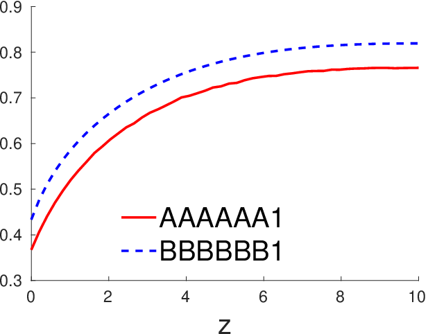
Finally, Fig. 6 shows the dramatic increase of the normalized correlation $\left|C^{(4)}(z)\right|/\sqrt{\left\langle I(z)\right\rangle\left\langle I^{(4)}(z)\right\rangle}$ with the penetration depth, up to $\approx 0.8$ at the slab exit.

References

- [1] L. L. Foldy, Phys. Rev. 67, 107 (1945).
- [2] M. Lax, Rev. Mod. Phys. 23, 287 (1951).
- [3] M. Lax, Phys. Rev. 85, 621 (1952).
- [4] M. P. Van Albada and A. Lagendijk, Phys. Rev. Lett. 55, 2692 (1985).
- [5] P.-E. Wolf and G. Maret, Phys. Rev. Lett. 55, 2696 (1985).
- [6] D. Wiersma, Nat. Phys. 4, 359 (2008).
- [7] V. E. Kravtsov, V. M. Agranovich, and K. I. Grigorishin, Phys. Rev. B 44, 4931 (1991).
- [8] M. Baudrier-Raybaut, R. Haidar, P. Kupecek, P. Lemasson, and E. Rosencher, Nature 432, 374 (2004).
- [9] X. Wen, S. Chen, and D. D. Dlott, J. Opt. Soc. Am. B 8, 813 (1991).
- [10] J. F. de Boer, A. Lagendijk, R. Sprik, and S. Feng, Phys. Rev. Lett. 71, 3947 (1993).
- [11] C. Vanneste and P. Sebbah, Phys. Rev. Lett. 87, 183903 (2001).
- [12] H. Cao, J. Y. Xu, D. Z. Zhang, S. H. Chang, S. T. Ho, E. W. Seelig, X. Liu, and R. P. H. Chang, Phys. Rev. Lett. 84, 5584 (2000).
- [13] T. Wellens and B. Grémaud, Phys. Rev. Lett. 100, 033902 (2008).
- [14] T. Wellens and B. Grémaud, Phys. Rev. A 80, 063827 (2009).
- [15] N. A. Kurnit, I. D. Abella, and S. R. Hartmann, Phys. Rev. Lett. 13, 567 (1964).
- [16] I. D. Abella, N. A. Kurnit, and S. R. Hartmann, Phys. Rev. 141, 391 (1966).
- [17] T. W. Mossberg, Opt. Lett. 7, 77 (1982).
- [18] V. Markushev, N. Ter-Gabriélyan, C. Briskina, V. Belan, and V. Zolin, Quantum Electron. 20, 773 (1990).
- [19] M. Colice, F. Schlottau, K. Wagner, R. Mohan, W. Babbitt, I. Lorgeré, and J.-L. Le Gouët, in Proceedings of SPIE, Vol. 5557 (2004) p. 132.
- [20] J.-L. Le Gouët, F. Bretenaker, and I. Lorgeré, in Advances In Atomic, Molecular, and Optical Physics, Vol. 54, edited by P. R. Berman, C. C. Lin, and E. Arimondo (Elsevier, 2007) pp. 549–613.
- [21] W. Tittel, M. Afzelius, R. Cone, T. Chanelière, S. Kroll, S. Moiseev, and M. Sellars, Laser & Photon. Rev. 1, 1863 (2009).
- [22] H. de Riedmatten, M. Afzelius, M. U. Staudt, C. Simon, and N. Gisin, Nature 456, 773 (2008).
- [23] F. Beaudoux, A. Ferrier, O. Guillot-Noël, T. Chanelière, J.-L. Le Gouët, and P. Goldner, Opt. Express 19, 15236 (2011).
- [24] A. Perrot, P. Goldner, D. Giaume, M. Lovrić, C. Andriamiadamanana, R. R. Gonçalves, and A. Ferrier, Phys. Rev. Lett. 111, 203601 (2013).
- [25] T. W. Mossberg, R. Kachru, S. R. Hartmann, and A. M. Flusberg, Phys. Rev. A 20, 1976 (1979).
- [26] V. E. Kravtsov, V. M. Agranovich, and K. I. Grigorishin, Phys. Rev. B 44, 4931 (1991).
- [27] T. Ito and M. Tomita, Phys. Rev. E 69, 036610 (2004).
- [28] S. E. Skipetrov, J. Opt. Soc. Am. B 21, 168 (2004).
- [29] M. C. W. van Rossum and T. M. Nieuwenhuizen, Rev. Mod. Phys. 71, 313 (1999).
- [30] E. Akkermans and G. Montambaux, Mesoscopic Physics of Electrons and Photons (Cambridge University Press, Cambridge, 2007).
- [31] U. Frisch, La propagation des ondes en milieu aléatoire et les équations stochastiques (Institut d’Astrophysique, 1967).
- [32] F. Dyson, Phys. Rev. 75, 486 (1949a).
- [33] F. Dyson, Phys. Rev. 75, 1736 (1949b).
- [34] S. M. Rytov, Y. A. Kravtsov, and V. I. Tatarskii, Principles of Statistical Radiophysics, Vol. 4 (Springer-Verlag, Berlin, 1989).
- [35] L. A. Apresyan and Y. A. Kravtsov, Radiation Transfer: Statistical and Wave Aspects (Gordon and Breach Publishers, Amsterdam, 1996).
- [36] A. Ishimaru, Wave Propagation and Scattering in Random Media (IEEE Press, Oxford, 1997).
- [37] S. Chandrasekhar, Radiative Transfer (Dover, New-York, 1950).