Investigating the Metallicity–Mixing Length Relation

Each star in this study has observed measurements of $\nu_{\mathrm{max}}$, $\Delta\nu$, $T_{\mathrm{eff}}$, and $\mathrm{[Fe/H]}$. $\nu_{\mathrm{max}}$ is the frequency at which the oscillation power is at a maximum and can be approximately related to a star’s surface gravity and effective temperature as $\nu_{\mathrm{max}}\propto gT_{\mathrm{eff}}^{-1/2}$ [8, 33, 5]. $\Delta\nu$, the large frequency separation, is the average frequency spacing between adjacent radial order ($n$) modes of the same degree ($\ell$). $\Delta\nu$ is approximately related to a star’s average density by $\Delta\nu\propto\sqrt{\bar{\rho}}$ [62, 69, 10, 11, see, e.g.,]. The seismic data was obtained from [56], who added 415 subgiant and dwarf stars to the original APOKASC catalog [51] and determined $\Delta\nu$ and $\nu_{\mathrm{max}}$ values from Kepler lightcurves. The $\mathrm{[Fe/H]}$ values were obtained from the spectroscopic survey of [9]. [9] observed the stars with the Tillinghast Reflector Echelle Spectrograph using the 1.5 m Tillinghast Reflector. The $T_{\mathrm{eff}}$ values were determined from these spectra in an iterative process after fixing $\log g$ to seismic values and can be found in [44]. These stars and their properties can be seen in Table 3.

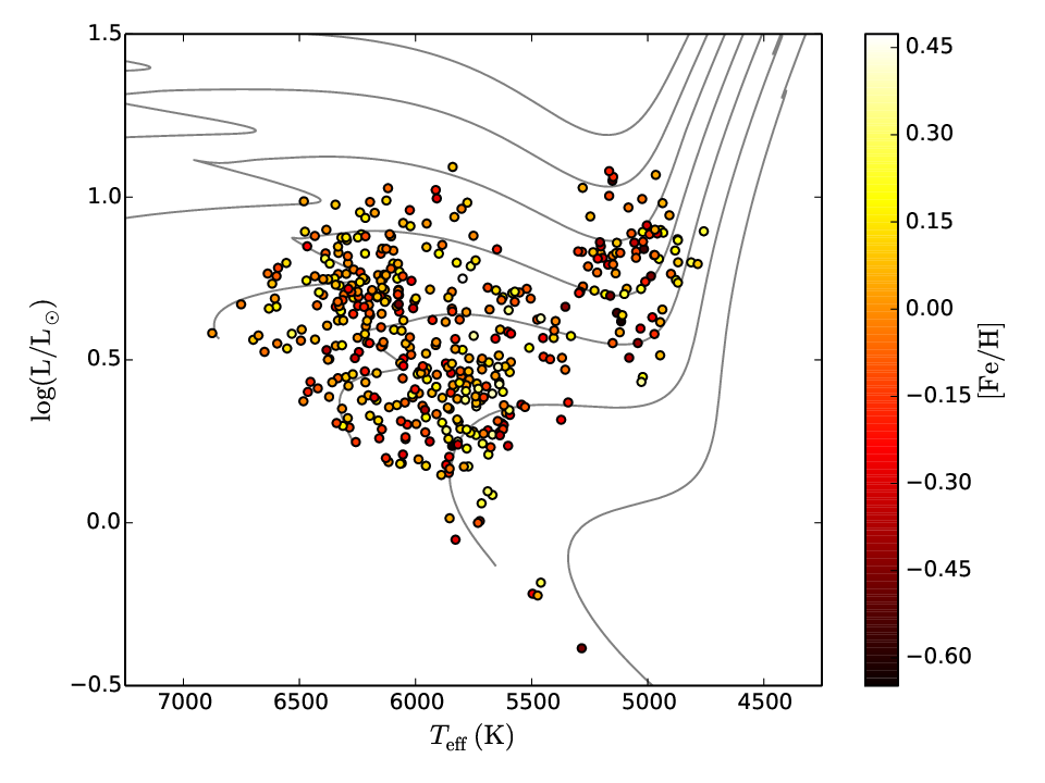
Figure 1 shows the H-R diagram with the stars in this work included, for the non-diffusion models. The background gray lines show tracks of 0.8, 1.0, 1.2, 1.4, 1.6, 1.8, and 2.0 $M_{\sun}$, generated using YREC [19], for reference. The values of $T_{\mathrm{eff}}$ and $L$ are from the likelihood weighted average values of the models (as explained in Sec. II.4). The points are colored by their likelihood weighted average value of $\mathrm{[Fe/H]}$.

Each star in our sample was modeled using the Yale stellar evolution code YREC [19]. All models were created with the OPAL equation of state [52] and OPAL opacities [31] supplemented with low temperature opacities from [23]. Nuclear reaction rates from [1] were adopted, except for that of the ${}^{14}N$($p$,$\gamma$)${}^{15}O$ reaction, for which we used the rates of [25]. Models were constructed with Eddington gray atmospheres.

The core set of models include core overshoot with an extent of $0.2H_{p}$. We did construct a subset of models without core overshoot as well. We made two full sets of models, the first of which did not include the diffusion and gravitational settling of helium and other heavy elements. These “No Diffusion” models form the core of our investigation. The second set of models were constructed including diffusion and gravitational settling using the rates of [64]. However, in hot stars, diffusion as modeled is known to drain out heavy elements quickly and to avoid this we multiplied the diffusion rate by a mass-dependent factor given by

Eq. 1 serves to smoothly decrease the diffusion rate for higher mass stars. The need to use this rather arbitrary factor is why we use the non-diffusion models as our primary set.

The $\Delta Y/\Delta Z$ relation was determined by constructing standard solar models. For models without diffusion, a calibrated solar model implied $Y=0.248+1.0958Z$, where we assumed that the primordial helium abundance $Y_{p}=0.248$. For models with diffusion, we get $Y=0.248+1.4657Z$. We use the metallicity scale of [27] to convert [Fe/H] to $Z/X$. Note that the solar calibrated mixing length is 1.70098 for models without diffusion and 1.838417 for models with diffusion.

The starting point of modeling each star was the input $\Delta\nu$, $\nu_{\rm max}$, $T_{\rm eff}$ and [Fe/H]. Since each of these quantities is associated with an uncertainty, we created many more realizations of these parameters to obtain a larger set of ($\Delta\nu$, $\nu_{\rm max}$, $T_{\rm eff}$, [Fe/H]), however, in each case the uncertainty was assumed to be 1.5 times larger than the quoted uncertainties in the data to obtain a larger range of inputs, this was particularly important in order to ensure that surface term effects on $\Delta\nu$ and $\nu_{\rm max}$ do not bias the calculations at this stage. Each realization of the inputs was then used to calculate mass $M$ and radius $R$ of the models using the modified $\Delta\nu$ relation proposed by [30] and the usual $\nu_{\rm max}$ scaling relation [33]. Note that the scaling relations here are used simply to determine a model mass and radius for each realization. When actually analyzing the models and determining model likelihoods (see Sec. II.4) the scaling relations are not used, as individual model frequencies are calculated instead, as will be described shortly. Models were constructed for each ($M$, $R$, $T_{\rm eff}$, [Fe/H]) realization. This was done by running YREC in an iterative manner by allowing the the mixing length parameter $\alpha$ to vary until we constructed a model of the required radius at the required $T_{\rm eff}$ for the given mass and metallicity.

We calculated the $\ell=0$ mode frequencies for each model. These were then used to determine the large separation $\Delta\nu$ as an average of the large separation weighted by the observed power envelope which is a Gaussian with a FWHM of $0.66\nu_{\rm max}^{0.88}$ [50]. The obtained $\Delta\nu$ was corrected for surface-term effects using the factor determined in Section II.3. For each model $\nu_{\rm max}$ was calculated from the acoustic cutoff using the prescription of [70]. The surface-term corrected $\Delta\nu$, $\nu_{\rm max}$, $T_{\rm eff}$ and [Fe/H] were then used to calculate the likelihood for each model (Section II.4).

We used a minimum of 500 realizations, though most stars needed more. The number of realizations was determined by determining $\alpha$ after every ten runs beyond the initial 500, and determining if the likelihood weighted average of $\alpha$ (see Section II.4) converged. Note that our procedure was different from that of [7], who first determined $M$ and $R$ from a grid-based modeling exercise and then did a Monte Carlo over the derived ($M$, $R$, $T_{\rm eff}$, [Fe/H]). We realized that the old procedure could lead to models that do not satisfy the input $\Delta\nu$ and $\nu_{\rm max}$.

When using frequencies of stellar models, the so-called “surface term” [12], a frequency difference between observed frequencies and frequencies from stellar models, must be considered and corrected. The surface term has been found to be a function of frequency once corrected for the mode-inertia [12]. These frequency differences arise due to the difficulties in modeling convection and the upper layers of stars. This therefore means that the surface term is also model dependent and is affected by the model physics [13, 21]. Many different methods of correcting for the surface term exist, for example modeling the surface term as a power law, using a scaled version of the solar surface term, as well as more complicated methods [34, 28, 2, 57, e.g., see]. An extensive comparison of these methods are discussed in more detail in [54]. For individual frequency modes, [2] show that the frequency shift can be approximated well with the function form,

where $\delta\nu$ is the frequency shift, $\mathcal{I}$ is the normalized mode inertia, $\nu_{\mathrm{ac}}$ is the acoustic cutoff frequency, and $a_{-1}$ and $a_{3}$ are the coefficient variables to be fit.

Since one of the stellar parameters these models will be fit to is $\Delta\nu$, some type of surface term correction must be applied in order to get correct results. In other words, we must determine how the surface correction effects our model measurements of $\Delta\nu$. A comparison of the value of $\Delta\nu$ determined from stellar models and from observations was performed for two different data sets. The first data set, from [40], consisted of observed mode frequencies from the Kepler LEGACY sample. These Kepler LEGACY sample stars had also previously been modeled using YREC for use in [58]. For these models the individual mode frequencies were determined using the “Yale Monte Carlo Method” (YMCM) described in [57] with some slight modifications as explained in [58]. Models for these Kepler LEGACY sample stars were created both with and without diffusion. The second data set has observed oscillation modes from Kepler from [16]. Model frequencies were obtained using the YMCM with models from [57]. For this set, only stars with measured $\nu_{\mathrm{max}}$ values were included.

For each stellar model, the [2] surface term correction (Eq. 2) could be applied. Since the individual mode frequencies were computed for each model and the corresponding observed frequencies were known from the literature sources mentioned, the coefficients $a_{-1}$ and $a_{3}$ were solved for each star by implementing a two-term unweighted least-$\chi^{2}$ fit. The surface term corrected frequencies for the stellar models were then compared to the observed frequencies to determine which stellar models were the best for each star.

Then, for each set of models $\Delta\nu$ was calculated for each star. For the model stars the large frequency separation was calculated by taking the individual mode frequencies for the $\ell=0$ modes and the corresponding radial quantum number ($n$) and using a weighted least-squared linear fit with Gaussian weights centered around $\nu_{\mathrm{max}}$ with a FWHM of $0.66\nu_{\mathrm{max}}^{0.88}$ as described in [50]. The fractional difference between the model calculated value of $\Delta\nu$ and the observational value of $\Delta\nu$ for each model was then calculated where $\delta(\Delta\nu)/\Delta\nu=(\Delta\nu_{\mathrm{model}}-\Delta\nu_{\mathrm{obs}})/\Delta\nu_{\mathrm{obs}}$. This fractional difference between $\Delta\nu$ from the models and from the observed data can be seen in Fig. 2.

From the values of $\delta(\Delta\nu)/\Delta\nu$ we can estimate the factor by which our model value of $\Delta\nu$ differs from the observed value of $\Delta\nu$. Based on the data in Fig. 2, for the error-weighted average for all the models together we obtain $\delta(\Delta\nu)/\Delta\nu=0.0109$. This means that

and so using Eq. 3 the surface term effects on $\Delta\nu$ can be removed and we can have confidence in comparing our model $\Delta\nu$ values to the observed $\Delta\nu$ values of our sample stars.

For each star, the Monte Carlo simulations resulted in typically 2-3 thousand stellar models. For each model, likelihood values for $\Delta\nu$, $\nu_{\rm max}$, $T_{\rm eff}$, and $\mathrm{[Fe/H]}$, were computed. These likelihood values were calculated following the form of Eq. 4, using $\Delta\nu$ as an example.

where $\Delta\nu_{\mathrm{model}}$ is the model’s value of $\Delta\nu$, $\Delta\nu_{\mathrm{obs}}$ is the observed value of $\Delta\nu$ from [56], and $\sigma_{\mathrm{\Delta\nu}}$ is the uncertainty in the observed value of $\Delta\nu$. Likelihood values for $\Delta\nu$, $\nu_{\rm max}$, $T_{\rm eff}$, and $\mathrm{[Fe/H]}$, were calculated in this manner. Note that before calculating the value of $\mathcal{L}_{\Delta\nu}$ the model values of $\Delta\nu$ were corrected for the surface term as explained in Sec. II.3.

A weighting factor for the age of the models was also included, with the purpose to ensure that models older than the age of the universe were given lower weights. The age weighting factor, $\mathcal{W}_{\mathrm{age}}$, is given by

where the age of the universe is 13.8 Gyr and $\sigma_{\mathrm{Age_{\mathrm{Universe}}}}=0.1$ Gyr. The value of $\sigma_{\mathrm{Age_{\mathrm{Universe}}}}$ was chosen such that the weighting function smoothly and quickly goes to zero for high ages (as can be seen in Fig. 3).

The total likelihood for each model was determined by multiplying the individual likelihood values together, so that

With the likelihood of each model for a given star determined, the likelihood weighted average of model quantities was calculated following the form of Eq. 7, using mass as an example,

with the likelihood weighted uncertainty being

where $N$ is the number of models for each star. Using Eq. 7 and 8 the value of stellar properties, such as mass, radius, age, temperature, $\mathrm{[Fe/H]}$, and $\alpha$ were calculated for each star. The process was also recalculated, for later use (see Sec. III.5), excluding the $\nu_{\rm max}$ likelihood values in Eq. 6 so that the total likelihood was only determined by the $\Delta\nu$, $T_{\rm eff}$, $\mathrm{[Fe/H]}$, and age values.

For each star the probability density function (PDF) for $\alpha$, that was obtained by marginalizing over all other parameters, was also examined to ensure the models converged properly. Several examples of the different types of PDFs (symetric, bimodal, skewed, and wide) for $\alpha$ can be seen in Figures 4-7. These figures show the smoothed continuous PDF functions. An example of the discrete PDF can be seen in the first panel of Fig. 4 (the gray background histogram). The discrete PDFs were transformed into the smoothed continuous PDFs using a kernel density estimation (KDE), where the bandwidth was determined using Scott’s rule [55]. Note that the stellar properties were not determined from the PDFs but from the likelihood weighted averages.

Following the work of [7], we are interested in examining the relationship between the mixing length parameter and a star’s metallicity. First we will examine the non-diffusion, $0.2H_{p}$ set of stellar models and in later sections we report the result of the analysis for the other sets of models. Since we will later be comparing the results to models with diffusion, it is best to use the quantity $\alpha/\alpha_{\sun}$ to compare the results of the different model physics. As mentioned earlier, in the non-diffusion case the value of $\alpha_{\sun}$ is $1.70098$ and for the diffusion models $\alpha_{\sun}$ is $1.838417$. The analysis is performed on stars with likelihood weighted $\alpha$ of $<4$, as the results for stars with $\alpha>4$ are rather unstable and thus not included. For the 460 stars modeled in this work, only 7 had average likelihood weighted values of $\alpha>4$. The high $\alpha$ values for the handful of excluded stars arose due to the models not properly converging in those cases.

As in the analysis of [7], we perform a trilinear fit to model $\alpha/\alpha_{\sun}$ as a function of $\log(g)$, $\log(T_{\mathrm{eff}})$, and $\mathrm{[Fe/H]}$. Our equation takes the form,

Using a minimum $\chi^{2}$ fit, the coefficients $a$, $b$, $c$, and $d$ for Eq. 9 were determined, with the results displayed in Table 1. Fig. 8 shows the residuals and partial residuals for this fit. We find a positive trend between $\alpha/\alpha_{\sun}$ and $\mathrm{[Fe/H]}$, a negative trend between $\alpha/\alpha_{\sun}$ and $\log(T_{\mathrm{eff}})$, and a slightly negative trend between $\alpha/\alpha_{\sun}$ and $\log(g)$.

The best-fit coefficients to Eq. 9 for this work are compared to those found in [7] in Table 2. Note that the coefficients presented in [7] were for a fit to $\alpha$ and not $\alpha/\alpha_{\sun}$. To make the comparison with our results more clear, the [7] values in Table 2 have been divided by the value of $\alpha_{\sun}$ from [7]. For each of the coefficients the sign is the same, however most notably the metallicity dependence from this work is larger. This is likely to be a result of the larger $\log g$ range and coverage of the current sample.

The properties of the stars in this study are shown in Table 3. The values of $\nu_{\mathrm{max}}$ and $\Delta\nu$ were obtained from [56], the $T_{\mathrm{eff}}$ values are from [44], the $\mathrm{[Fe/H]}$ values are from [9], and the $\alpha$ values are the likelihood weighted average values for the non-diffusion, $0.2H_{p}$ models.

For the non-diffusion, $0.2H_{p}$ set of models, we also re-compute the trilinear fit (Eq. 9) for 3 different temperature ranges, $\log(T_{\mathrm{eff}})<3.73$, $3.73<\log(T_{\mathrm{eff}})<3.78$, and $\log(T_{\mathrm{eff}})>3.78$. The partial residuals with respect to $\mathrm{[Fe/H]}$ for these temperature divisions can be seen in Fig. 9 and the values of the fit coefficient can be found in Table 4. While the temperature range does affect the fit coefficients, we still see a positive correlation between $\alpha$ and $\mathrm{[Fe/H]}$ in each range with the coefficient being between 0.328 and 0.605.

We also test the impact of using a different temperature scale. The model likelihoods were recalculated, where $\mathcal{L}_{T_{\mathrm{eff}}}$ was determined using the ASPCAP $T_{\mathrm{eff}}$ values from [56]. The trilinear fit was recomputed and the resulting $\mathrm{[Fe/H]}$ coefficient was 0.438 $\pm$ 0.031, compared to the original value of 0.437 $\pm$ 0.029 when using the original temperatures. So, the $\mathrm{[Fe/H]}$ coefficients are in excellent agreement.

We can also separate the stars by their evolutionary phase. Looking at the residuals from Fig. 8, the partial residuals for $T_{\mathrm{eff}}$ and $\log g$ appear to have different trends at low $T_{\mathrm{eff}}$ and low $\log g$, the more evolved stars, than compared to the partial residuals at higher $T_{\mathrm{eff}}$ and $\log g$. We can investigate if this is the result of a relation between the best fit coefficients, $\alpha$, and evolutionary phase. Fig. 10 plots the stars on the $\log g-T_{\mathrm{eff}}$ plane. As can be seen in Fig. 10, there is a distinct group of stars which are more evolved. This group of more evolved stars can also be seen in the H-R diagram in Fig. 1. We perform the trilinear analysis separately on the group of more evolved and less evolved stars to examine how the fit coefficients change, recorded in Table 5. Separating the stars into those which are more evolved and those which are less evolved does remove the features in the partial residuals at low $T_{\mathrm{eff}}$ and $\log g$. For the more evolved stars the $\mathrm{[Fe/H]}$ coefficient decreased while in the less evolved stars the trend with $\mathrm{[Fe/H]}$ increased. Additionally, for the more evolved stars, the $\log(T_{\mathrm{eff}})$ and $\log g$ coefficients changed sign.

An examination of the PDF and model likelihood results for each star shows that some stars have bimodal distributions both in mass and $\alpha$. An example of such a PDF is that of KIC 2010607, which is shown in Fig. 11. In these cases, the lower mass peak corresponds to the higher $\alpha$ peak and vice versa. This can be seen in Fig. 12. About 5% of the stars have such a bimodal distribution in both mass and $\alpha$.

In these cases, a bimodal Gaussian function was fit to the PDF histogram to determine the value of each peak and the corresponding $\sigma$. The star was then treated as having two separate solutions, one for each set of mass and $\alpha$ peaks. We can examine how separating the peaks effects the results compared to the original values for the non-diffusion, $0.2H_{p}$ models. With the bimodal stars split the $\mathrm{[Fe/H]}$ coefficient is 0.528 $\pm$ 0.034 and with the bimodal stars removed from the sample the $\mathrm{[Fe/H]}$ coefficient is 0.436 $\pm$ 0.030, compared to the original $\mathrm{[Fe/H]}$ coefficient of 0.437 $\pm$ 0.029.

The procedure was repeated with several other sets of stellar models, all with unique model physics. The additional sets were models including diffusion, a set of models without diffusion and without overshoot, and a recalculation of the original non-diffusion, $0.2H_{p}$ models without the inclusion of the $\mathcal{L_{\nu_{\mathrm{max}}}}$ term in the likelihood calculation. For each set of stellar physics, the best fit values for the coefficients in the trilinear fit of Eq. 9 are shown in Table 6. The residuals and partial residuals for the other sets of models can be seen in Figs. 13 and 14. In all cases, the linear model agrees well with the data. It is interesting to note that the $\mathrm{[Fe/H]}$ coefficients for the different model sets are in agreement with each other while the $\log g$ and $\log(T_{\mathrm{eff}})$ coefficients are not. The $\log(T_{\mathrm{eff}})$ coefficient changes in magnitude fairly substantially and the $\log g$ coefficient changes in sign depending on the model physics while the correlation with $\mathrm{[Fe/H]}$ appears to be more model independent.

If the value of $\alpha$ does depend on the metallicity of the star, then for a given metallicity the temperature-luminosity relation changes. This in turn will change the isochrones, especially on the giant branch, as mentioned in [18], for example. [72] explains that since a larger $\alpha$ makes convection more efficient, then the stellar model will be bluer and hotter. This color uncertainty can cause age uncertainties of 25% [72].

To demonstrate the effects that a metallicity dependent $\alpha$ has on stellar isochrones, isochrones were created for metallicities of $\mathrm{[Fe/H]}=-0.5$ and $+0.5$ for the non-diffusion, $0.2H_{p}$ set of models. For each metallicity two sets of isochrones were created in YREC, one set with the solar calibrated value of $\alpha$, and one set with the value of $\alpha$ following the trend observed between $\alpha$ and $\mathrm{[Fe/H]}$. The $\mathrm{[Fe/H]}=-0.5$ isochrones are 8 Gyr while the $\mathrm{[Fe/H]}=+0.5$ isochrones are 1 Gyr in age.

These isochrones can be seen in Fig. 16. As can be seen in Fig. 16, a smaller mixing length parameter shifts the isochrones towards cooler temperatures, agreeing with the explanation given by [72]. The clear difference between the sets of isochrones with different $\alpha$ values, especially at turn-off and the giant branch, show the importance of correctly selecting the value of the mixing length parameter as opposed to relying on the the solar calibrated value.

It is also possible that the relationship between $\alpha$, $T_{\rm eff}$, $\log g$, and $\mathrm{[Fe/H]}$ is not a linear one, but takes on some other functional form. To investigate this, the software package Eureqa [53] was used. Eureqa, available from the Nutonian company, performs symbolic regression through the use of an evolutionary search. The evolutionary search found that for the non-diffusion, $0.2H_{p}$ models the best fit took the form,

We can compare the linear fit from Eq. 9 to this more complicated equation, as seen in Fig. 17, which shows the total residuals, $(\alpha/\alpha_{\sun})_{\mathrm{Model\>Stars}}-(\alpha/\alpha_{\sun})_{\mathrm{Equational\>Fits}}$.

From Fig. 17, the Eureqa functional form and the linear model residuals do not appear significantly different. It is worth noting that in the low temperature region the Eureqa model residuals are much closer to zero compared to the residuals for the linear model. Comparing the reduced $\chi^{2}$ values for the linear model and the Eureqa equation we find that $\chi_{\mathrm{Linear}}^{2}=1.333$ and $\chi_{\mathrm{Eureqa}}^{2}=0.615$. While the $\chi^{2}$ value is about a factor of 2 better, the complicated form of Eq. 10 does not appear to be justified on any theoretical basis. While the trilinear fit is not either, it is at least a simple equational form which provides a good fit.

The inclusion of a $\log(M)$ term in Eq. 9 was also tested. A quadrilinear fit including $\log(T_{\mathrm{eff}})$, $\log(g)$, $\mathrm{[Fe/H]}$, and $\log(M)$ was performed for the non-diffusion, $0.2H_{p}$ models. The resulting fit coefficient for the $\mathrm{[Fe/H]}$ term was 0.463 $\pm$ 0.039 for the quadrilinear fit, compared to 0.437 $\pm$ 0.029 for the trilinear fit without the $\log(M)$ term. The reduced $\chi^{2}$ for the quadrilinear fit was 1.335, compared to 1.333 for the trilinear fit.

The analysis for the non-diffusion, $0.2H_{p}$ models was also repeated using principal component analysis (PCA). PCA was used to transform the variables $\log g$, $\mathrm{[Fe/H]}$, and $\log(T_{\mathrm{eff}})$ into three orthogonal principal components in the directions of the the greatest variance. These three principal components were then fit linearly to $\alpha/\alpha_{\odot}$. The resulting fit, when converted back to the original variables instead of the principal components, gives the same fit coefficients as previously determined using the original linear fit.

Our results can be compared to other works in literature. [63] compared stellar models and stars in the APOKASC sample [51], finding a metallicity dependent temperature offset. [63] demonstrated that a metallicity dependent mixing length, of the form, $\alpha=0.1612\mathrm{[Fe/H]}+1.9037$ improves the differences. For the sake of comparison we divide the [63] correction by their value of $\alpha_{\sun}$ so that $\alpha/\alpha_{\sun}=0.0937\mathrm{[Fe/H]}+1.1068$. For our sample, the line of best fit for $\alpha/\alpha_{\sun}$ as a function of $\mathrm{[Fe/H]}$ gives: $\alpha/\alpha_{\sun}=0.437\mathrm{[Fe/H]}+1.029$. So, we find a much stronger metallicity dependence in this set of stars. However, [63] performed their analysis on red giant stars, while our sample consists of mainly dwarfs and subgiants. As demonstrated in Sec. III.3, the trend between $\alpha$ and $\mathrm{[Fe/H]}$ is weaker in more evolved stars. So, we would expect the $\mathrm{[Fe/H]}$ coefficient for the [63] red giant stars to be smaller compared to this sample. Taking only the more evolved stars in this work (see Fig. 10) then the line of best fit is: $\alpha/\alpha_{\sun}=0.292\mathrm{[Fe/H]}+1.109$.

[47] modeled 42 Kepler target stars using the Asteroseismic Modeling Portal [45, 71] and found a negative correlation between $\alpha$ and $T_{\mathrm{eff}}$ and a positive trend between $\alpha$ and $\mathrm{[Fe/H]}$ and $g$. Additinally, [15] modeled 57 stars using the Asteroseismic Modeling Portal and also found a positive trend between $\alpha$ and metallicity as well as between $\alpha$ and $\log g$ and a negative trend between $\alpha$ and $\log(T_{\mathrm{eff}})$. This trend between $\alpha$ and $T_{\mathrm{eff}}$ and $\mathrm{[Fe/H]}$ agrees with our results, however the trend with surface gravity does not. This, however, could be a result of the larger range of $\log g$ in our sample. If our range of $\log g$ is restricted to the same range as [15] then we also see a positive correlation between $\alpha$ and $\log g$ and $\alpha$ and metallicity with a negative trend between $\alpha$ and $T_{\rm eff}$.

It is much more interesting to compare these results with those obtained from 3D simulations. However, the complicating issue there is that defining $\alpha$ for a 3D simulation is difficult, and the definitions are ambiguous given that 3D simulations show that convection looks nothing like the MLT picture of overturning eddies of a given size. Nonetheless, there have been attempts to define $\alpha$ from the simulations. [42] did a grid of 3D radiative hydrodynamic simulations of convection at different $\log g$, $T_{\rm eff}$, and metallicity and produced three different types of $\alpha$ that we could fit to Eq. 9 and compare to our results. The three $\alpha$ values that [42] produced are $\alpha_{\mathrm{MLT}}^{s_{\mathrm{bot}}}$, $\alpha_{\mathrm{MLT}}^{\Delta s}$, and $\alpha_{\mathrm{m}}$. As explained in [42], the two different forms of $\alpha_{\mathrm{MLT}}$ are computed and calibrated by matching $s_{\mathrm{bot}}$ or $\Delta s$ between the 1D and 3D models. Here $\Delta s$ is the entropy jump, defined as $\Delta s=s_{\mathrm{bot}}-s_{\mathrm{min}}$ and $s_{\mathrm{bot}}$ is the asymptotic entropy of the deep convective region. The third $\alpha$ value, $\alpha_{\mathrm{m}}$, is the mass mixing length, which [42] define as the inverse gradient of the vertical mass flux. We then perform the trilinear fit to our Eq. 9 and compare the coefficients for these different $\alpha$ values to our results. The best-fit coefficient for each different $\alpha$ value can be seen in Table 7 where [42] is referred to as 42. Mixing length values of models were also obtained from [68] (henceforth 68), and the trilinear fit was also performed on these stars as well as on values of $\alpha_{\mathrm{m}}$ obtained from [67] (henceforth 67). The [67] and [68] models were all of solar metallicity, and hence the $\mathrm{[Fe/H]}$ coefficient in Eq. 9 is not determined for these cases.

As with the [63] comparison with simulations, the metallicity-dependence of our mixing length results show a disagreement when compared to “mixing lengths” obtained from 3D simulations of convection; the sign of the change is the opposite. The reasons are not completely clear. The real $T$–$\tau$ relation in stars is more complicated than the Eddington $T$–$\tau$ relation, but [61] showed that an $\alpha$ that increases with metallicity is also obtained when models are constructed with the $T$–$\tau$ relation obtained from convection simulations of the correct metallicity.

In addition to $\alpha$, [42] tabulate entropy too, which we fit to Eq. 9. Specifically, we fit the [42] values of $\Delta s/\Delta s_{\sun}$ and $s_{\mathrm{bot}}/s_{\mathrm{bot,\sun}}$, as well as the maximal rms entropy, $\delta s_{\mathrm{rms}}^{\mathrm{peak}}$, to Eq. 9. Additionally, entropy values from [66] (henceforth 66) were obtained. From [66] values of $S_{\mathrm{max}}$, the asymptotic entropy, and $S_{\mathrm{Jump}}$, the atmospheric entropy jump, were obtained. The [66] entropy values were also fit to Eq. 9. Note that the [66] models are all of solar metallicity, and so the metallicity coefficient cannot be determined for these models. The best-fit coefficients for the entropy values can be found in Table 7. Comparing the best-fit coefficients for the entropy values to the results of this work, it is interesting to note that the metallicity dependence of our $\alpha$ and the metallicity dependence of the 42 entropy measures have the same sign. However, since a larger $\alpha$ in models implies a smaller entropy jump, in essence the results are again in disagreement. It should be noted that mixing-length models ignore the effects of turbulent pressure — gas pressure alone supports gravity, this of course changes what would have been the entropy and thus comparing entropy may not be a fair comparison, particularly since the presence of turbulence effectively changes the equation of state.

[42] also had convective velocities. We performed the trilinear fit to the maximal rms velocity, $\delta v_{z,\mathrm{rms}}^{\mathrm{peak}}$, as well. The best-fit coefficients can be seen in Table 7. This is the only case where we see an agreement with the sign of the metallicity dependence. Under the mixing-length approximation, a larger $\alpha$ implies a larger velocity, and thus both convection simulations and mixing length models show larger velocities for larger metallicities. Larger convective velocities for higher metallicity simulations were also seen in the simulations of [60], implying that this is a robust feature of both convection simulations and mixing-length models.

Stars with observed values of $\nu_{\mathrm{max}}$, $\Delta\nu$, $T_{\mathrm{eff}}$, and $\mathrm{[Fe/H]}$ were modeled in YREC. The resulting likelihood weighted average stellar properties were compared to the mixing length parameter for each star. We found that for the non-diffusion, $0.2H_{p}$ set of models, a linear equation of the form $\alpha/\alpha_{\sun}=5.426-0.101\log(g)-1.071\log(T_{\mathrm{eff}})+0.437(\mathrm{[Fe/H]})$ best represented the relationship between $\alpha$ and the stellar parameters. This process was repeated for several sets of stellar model input physics. The signs of the best-fit coefficients for the linear model were all found to agree with [7]. The equational form of the relationship between $\log(g)$, $\log(T_{\mathrm{eff}})$, $\mathrm{[Fe/H]}$, and $\alpha$ was also explored using the Eureqa symbolic regression software. The results were also compared to values of $\alpha$ determined from 3D convection simulations, however the trends observed in this work did not fully agree with the relationships observed from the simulations. The impact of a metallicity dependent mixing length value was demonstrated through the creation of two sets of example isochrones, of $\mathrm{[Fe/H]}=-0.5\>\mathrm{and}\>+0.5$, constructed with both the solar mixing length and the metallicity dependent mixing length values from this work. The large effect that the mixing length parameter has on stellar models, combined with what we know about the shortcomings of assuming a solar calibrated mixing length, make understanding the relationship between $\alpha$ and stellar parameters, especially metallicity, vitally important. Further investigation into the disagreement between the results of this work and those from 3D convective simulations, especially the disagreement in the metallicity dependence of $\alpha$, is needed.

References

- [1] Adelberger, E. G., Austin, S. M., Bahcall, J. N., et al. 1998, Reviews of Modern Physics, 70, 1265
- [2] Ball, W. H., & Gizon, L. 2014, A&A, 568, A123
- [3] Basu, S., Chaplin, W. J., & Elsworth, Y. 2010, ApJ, 710, 1596
- [4] Basu, S., Verner, G. A., Chaplin, W. J., & Elsworth, Y. 2012, ApJ, 746, 76
- [5] Bedding, T. R., & Kjeldsen, H. 2003, PASA, 20, 203
- [6] Böhm-Vitense, E. 1958, ZAp, 46, 108
- [7] Bonaca, A., Tanner, J. D., Basu, S., et al. 2012, ApJ, 755, L12
- [8] Brown, T. M., Gilliland, R. L., Noyes, R. W., & Ramsey, L. W. 1991, ApJ, 368, 599
- [9] Buchhave, L. A., & Latham, D. W. 2015, ApJ, 808, 187
- [10] Christensen-Dalsgaard, J. 1988, in IAU Symposium, Vol. 123, Advances in Helio- and Asteroseismology, ed. J. Christensen-Dalsgaard & S. Frandsen, 295
- [11] Christensen-Dalsgaard, J. 1993, in Astronomical Society of the Pacific Conference Series, Vol. 42, GONG 1992. Seismic Investigation of the Sun and Stars, ed. T. M. Brown, 347
- [12] Christensen-Dalsgaard, J., & Berthomieu, G. 1991, Theory of solar oscillations, ed. A. N. Cox, W. C. Livingston, & M. S. Matthews (Tucson, AZ: Univ. Arizona Press), 401–478
- [13] Christensen-Dalsgaard, J., & Thompson, M. J. 1997, MNRAS, 284, 527
- [14] Chun, S.-H., Yoon, S.-C., Jung, M.-K., Kim, D. U., & Kim, J. 2018, ApJ, 853, 79
- [15] Creevey, O. L., Metcalfe, T. S., Schultheis, M., et al. 2017, A&A, 601, A67
- [16] Davies, G. R., Silva Aguirre, V., Bedding, T. R., et al. 2016, MNRAS, 456, 2183
- [17] Deheuvels, S., & Michel, E. 2011, A&A, 535, A91
- [18] Demarque, P., Green, E. M., & Guenther, D. B. 1992, AJ, 103, 151
- [19] Demarque, P., Guenther, D. B., Li, L. H., Mazumdar, A., & Straka, C. W. 2008, Ap&SS, 316, 31
- [20] Demarque, P., Guenther, D. B., & van Altena, W. F. 1986, ApJ, 300, 773
- [21] Dziembowski, W. A., Paterno, L., & Ventura, R. 1988, A&A, 200, 213
- [22] Eggenberger, P., Charbonnel, C., Talon, S., et al. 2004, A&A, 417, 235
- [23] Ferguson, J. W., Alexander, D. R., Allard, F., et al. 2005, ApJ, 623, 585
- [24] Fernandes, J., & Neuforge, C. 1995, A&A, 295, 678
- [25] Formicola, A., Imbriani, G., Costantini, H., et al. 2004, Physics Letters B, 591, 61
- [26] Gai, N., Basu, S., Chaplin, W. J., & Elsworth, Y. 2011, ApJ, 730, 63
- [27] Grevesse, N., & Sauval, A. J. 1998, Space Sci. Rev., 85, 161
- [28] Gruberbauer, M., Guenther, D. B., & Kallinger, T. 2012, ApJ, 749, 109
- [29] Guenther, D. B., & Demarque, P. 2000, ApJ, 531, 503
- [30] Guggenberger, E., Hekker, S., Basu, S., & Bellinger, E. 2016, MNRAS, 460, 4277
- [31] Iglesias, C. A., & Rogers, F. J. 1996, ApJ, 464, 943
- [32] Joyce, M., & Chaboyer, B. 2017, ArXiv e-prints, arXiv:1712.05082
- [33] Kjeldsen, H., & Bedding, T. R. 1995, A&A, 293, 87
- [34] Kjeldsen, H., Bedding, T. R., & Christensen-Dalsgaard, J. 2008, ApJ, 683, L175
- [35] Lastennet, E., Fernandes, J., Valls-Gabaud, D., & Oblak, E. 2003, A&A, 409, 611
- [36] Lattanzio, J. V. 1984, PhD thesis, Monash University, Australiathd
- [37] Lebreton, Y., Fernandes, J., & Lejeune, T. 2001, A&A, 374, 540
- [38] Ludwig, H.-G., Freytag, B., & Steffen, M. 1999, A&A, 346, 111
- [39] Ludwig, H.-G., & Salaris, M. 1999, in Astronomical Society of the Pacific Conference Series, Vol. 173, Stellar Structure: Theory and Test of Connective Energy Transport, ed. A. Gimenez, E. F. Guinan, & B. Montesinos, 229
- [40] Lund, M. N., Silva Aguirre, V., Davies, G. R., et al. 2017, ApJ, 835, 172
- [41] Magic, Z., Collet, R., Asplund, M., et al. 2013, A&A, 557, A26
- [42] Magic, Z., Weiss, A., & Asplund, M. 2015, A&A, 573, A89
- [43] Mathur, S., Metcalfe, T. S., Woitaszek, M., et al. 2012, ApJ, 749, 152
- [44] Mathur, S., Huber, D., Batalha, N. M., et al. 2017, ApJS, 229, 30
- [45] Metcalfe, T. S., Creevey, O. L., & Christensen-Dalsgaard, J. 2009, ApJ, 699, 373
- [46] Metcalfe, T. S., Chaplin, W. J., Appourchaux, T., et al. 2012, ApJ, 748, L10
- [47] Metcalfe, T. S., Creevey, O. L., Doğan, G., et al. 2014, ApJS, 214, 27
- [48] Miglio, A., & Montalbán, J. 2005, A&A, 441, 615
- [49] Morel, P., Provost, J., Lebreton, Y., Thévenin, F., & Berthomieu, G. 2000, A&A, 363, 675
- [50] Mosser, B., Elsworth, Y., Hekker, S., et al. 2012, A&A, 537, A30
- [51] Pinsonneault, M. H., Elsworth, Y., Epstein, C., et al. 2014, ApJS, 215, 19
- [52] Rogers, F. J., & Nayfonov, A. 2002, ApJ, 576, 1064
- [53] Schmidt, M., & Lipson, H. 2009, Science, 324, 81
- [54] Schmitt, J. R., & Basu, S. 2015, ApJ, 808, 123
- [55] Scott, D. W. 1992, Multivariate Density Estimation (New York: Wiley)
- [56] Serenelli, A., Johnson, J., Huber, D., et al. 2017, ApJS, 233, 23
- [57] Silva Aguirre, V., Davies, G. R., Basu, S., et al. 2015, MNRAS, 452, 2127
- [58] Silva Aguirre, V., Lund, M. N., Antia, H. M., et al. 2017, ApJ, 835, 173
- [59] Straka, C. W., Demarque, P., & Guenther, D. B. 2005, ApJ, 629, 1075
- [60] Tanner, J. D., Basu, S., & Demarque, P. 2013, ApJ, 767, 78
- [61] —. 2014, ApJ, 785, L13
- [62] Tassoul, M. 1980, ApJS, 43, 469
- [63] Tayar, J., Somers, G., Pinsonneault, M. H., et al. 2017, ApJ, 840, 17
- [64] Thoul, A. A., Bahcall, J. N., & Loeb, A. 1994, ApJ, 421, 828
- [65] Trampedach, R. 2007, in American Institute of Physics Conference Series, Vol. 948, Unsolved Problems in Stellar Physics: A Conference in Honor of Douglas Gough, ed. R. J. Stancliffe, G. Houdek, R. G. Martin, & C. A. Tout, 141–148
- [66] Trampedach, R., Asplund, M., Collet, R., Nordlund, Å., & Stein, R. F. 2013, ApJ, 769, 18
- [67] Trampedach, R., & Stein, R. F. 2011, ApJ, 731, 78
- [68] Trampedach, R., Stein, R. F., Christensen-Dalsgaard, J., Nordlund, Å., & Asplund, M. 2014, MNRAS, 445, 4366
- [69] Ulrich, R. K. 1986, ApJ, 306, L37
- [70] Viani, L. S., Basu, S., Chaplin, W. J., Davies, G. R., & Elsworth, Y. 2017, ApJ, 843, 11
- [71] Woitaszek, M., Metcalfe, T., & Shorrock, I. 2009, in Proceedings of the 5th Grid Computing Environments Workshop, GCE ’09 (New York, NY, USA: ACM), 1:1–1:7
- [72] Yi, S. K. 2003, ApJ, 582, 202
- [73] Yıldız, M., Yakut, K., Bakış, H., & Noels, A. 2006, MNRAS, 368, 1941