subref name = section \RS@ifundefinedthmref name = theorem \RS@ifundefinedlemref name = lemma
Effective Connectivity from Single Trial fMRI Data by Sampling Biologically Plausible Models
Abstract
The estimation of causal network architectures in the brain is fundamental for understanding cognitive information processes. However, access to the dynamic processes underlying cognition is limited to indirect measurements of the hidden neuronal activity, for instance through fMRI data. Thus, estimating the network structure of the underlying process is challenging. In this article, we embed an adaptive importance sampler called Adaptive Path Integral Smoother (APIS) into the Expectation-Maximization algorithm to obtain point estimates of causal connectivity. We demonstrate on synthetic data that this procedure finds not only the correct network structure, but also the direction of effective connections from random initializations of the connectivity matrix. In addition–motivated by contradictory claims in the literature–we examine the effect of the neuronal time scale on the sensitivity of the BOLD signal to changes in the connectivity and on the maximum likelihood solutions of the connectivity. We conclude with two warnings: First, the connectivity estimates under the assumption of slow dynamics can be extremely biased if the data was generated by fast neuronal processes. Second, the faster the time scale, the less sensitive the BOLD signal is to changes in the incoming connections to a node. Hence, connectivity estimation using realistic neural dynamics time scale requires extremely high quality data and seems infeasible in many practical data sets.
1 Introduction
In recent years, the field of neuroimaging has seen a rapidly increasing interest in effective connectivity estimations from functional magnetic resonance imaging (fMRI) data. Although this data acquisition method is very powerful to investigate human brain function by identifying brain regions that are active during perceptual or cognitive tasks, fMRI time series are an indirect, delayed and blurred measurement of the actual signal of interest, the latent neuronal activation of a specific region of interest (ROI). Thus, estimating the underlying connectivity is challenging.
Roughly speaking there are two approaches to this problem based on the distinction between functional and effective connectivity. The first approach seeks to estimate the temporal correlations between separable ROIs [7]. Examples of these, which are known to correctly estimate the network structure, are partial correlation, regularized inverse covariance and some Bayes net methods [28].
These symmetric measures, however, have no information about the directionality of the connection, i.e. the influence that one node exerts over another. This "effective" connectivity is in general harder to estimate but it is often of great interest. We can distinguish between two families of approaches; purely data-driven methods that attempt to infer directionality directly from the time series using statistical measures and methods based on dynamic models that seek to find a forward model to fit the data.
Purely data-driven methods fall generally into three classes. First, lag-based methods, e.g. Granger causality [13, 12, 5], are variations of the well-known auto-regressive models. In this framework one considers the similarity between a pair of time series, one of which is shifted in time. If the lagged time series helps predict the zero-lagged time series, then a causal relation is inferred. A second family of methods is based on the concept of conditional independence and follow the ideas from structural learning in Bayes networks [14, 22]. The third class considers higher order statistics to infer causality. For instance, Patel’s approach measures the asymmetry between the conditional probabilities of functionally connected nodes. If the activation probability of a node given node is larger than the activation probability of node given node , this is interpreted as a directed connection [20]. Although many of these methods are widely used, the estimation of directed connectivity proves difficult with these methods [28].
Dynamic model methods frame the inference problem as a state-space model (SSM). The latent states are the dynamic degrees of freedom of the process underlying the data. Hence, in general, estimating the parameters of the model requires also the estimation of the hidden process, which is in most cases analytically infeasible and some approximations are needed. Once the latent process estimation is addressed, one typically uses the Expectation-Maximization (EM) algorithm in either its Maximum-Likelihood (ML) or variational Bayes versions [26, 25].
For fMRI data, model-based methods usually distinguish themselves in the approximations they make of the dynamic system or the latent process estimation (E-step). For instance, in [25] the fMRI time series is modeled as a linear convolution of the bi-linear latent system with the canonical hemodynamic response function (HRF) and its time derivative [21]. This approximation allows using the Kalman smoother for the E-step.
On the contrary, dynamic causal modeling (DCM) uses a biologically plausible nonlinear model for the hidden process. Here, the neuronal activity is given as a bi-linear system coupled to the Balloon model describing the nonlinear relation between blood flow and volume [2, 18, 10]. In addition, the fMRI observations are modeled as a nonlinear function of the hidden variables. Hence, to deal with the nonlinearities of the biological model, DCM resorts to either a Volterra expansion of the dynamic system or the generalized filtering method [8, 6, 9].
In addition, DCM uses a Gaussian approximation of the posterior over the parameters and its mean and covariance are estimated using EM update rules. For this, the adjacency matrix is specified beforehand, effectively imposing a strong prior on the connectivity of the system. Using the log-evidence, the proposed models are scored to find the best model amongst them [9]. Although DCM has been widely used, concerns about this approach have spurred a discussion about its feasibility and validity due to the combinatorial explosion of the network structure and the apparent inability of the scoring procedure to distinguish between generally accepted networks and randomly generated ones [17, 1, 4].
In this article, we present an alternative method for connectivity estimation. Our approach is similar to DCM in the sense that it uses the same model but differs in two important ways. First of all, in the E-step the full posterior over the latent process is estimated using an optimal control approach that was first introduced in [23]. Second, in the M-step the connectivity is optimized without prior assumptions as in [9, 8]. The Monte Carlo estimates involved in these steps are the only approximations required and it is proven to work for nonlinear deconvolution of fMRI time series [24].
We show using synthetic data that the connectivity estimates obtained are close to the ground truth and that adding a small L1-regularization on the connections is beneficial to obtain sparse estimates that generalize better on unseen time series. Furthermore, the proposed method obtains estimates from single event fMRI time series that are robust against random initializations of the connectivity matrix.
In addition, we study the sensitivity of the BOLD signal depending on the neuronal time scale and the effect of this parameter on the connectivity estimates. This analysis is motivated by the different claims about the value of the neuronal time scale in the literature. For instance, [28] used a time constant resulting in a mean neural lag of 50 ms and it is argued that this value is towards the upper limit of observed lags in general. Contrary to this claim is the assumption made in the DCM literature, where it is argued that the scale ought to be of order 1 s [8, 9].
We observe a significant effect of the neuronal time scale on the connectivity estimates and a remarkable lower sensitivity of the BOLD signal to changes in the connectivity for fast neuronal dynamics. Hence if the underlying neuronal processes are fast, the quality of the data must be significantly higher to obtain reliable, unbiased estimates of the effective connectivity.
2 Method
2.1 Modeling fMRI Data
Similar to DCMs [8], we consider the fMRI forward model as a network of regions that follow stochastic dynamics given by
| (1) |
where is a -dimensional Wiener process with variance11 1 In all our simulations we used this discretization step unless stated otherwise. and . The parameter sets the time scale of the neuronal response, while the connectivity matrix has diagonal with and off-diagonal elements . This form assumes that the fastest scale is the within-node temporal decay. The term in the diffusion ensures that the stationary distribution remains invariant under changes in the time scale . Contrary to DCMs, the input strength has been rescaled such that the stationary point of the system with non-zero constant input is independent of . Hence, the inverse time scale determines only how fast the neuronal system follows the input.
Notice that we define the process in () to have an unknown function . This function is the importance sampling controller learned with APIS. In general, can be any parametrized function [kappen2015adaptive], but in this paper it is chosen to have the simple form with a constant and a time varying function. We assume that the external input and its strength are known.
Each node’s activity is coupled to a nonlinear deterministic system modeling the hemodynamic transformation. For each node there are two Hemodynamic equations [10]
| (2) | ||||
and two equations of the Balloon model22 2 For clarity in the notation, we denote the exponent of the volume fraction simply as . [2],
| (3) | ||||
The BOLD signal change is given by
| (4) |
where , and denotes all parameters of the system. For simplicity, we assume the same hemodynamic transformation for all nodes since our focus is on connectivity estimates. The parameters are found in [10]. A summary of all the values used in this article is given in 1, unless a different value is stated explicitly. For now, we restrict our attention to slow neuronal processes with a neuronal lag of , which is around the typical values in the literature on effective connectivity, e.g. [8, 9]. The input strength is chosen such that the resulting amplitude of BOLD responses are around 2-4%.
| Parameter | Value | Parameter | Value | Parameter | Value | Parameter | Value |
|---|---|---|---|---|---|---|---|
| 1 Hz | |||||||
| 0.8 | 0.4 | 0.32 | |||||
| 1.54 | 0.018 | TBD | |||||
| TBD | |||||||
In addition, we consider for the prior over the initial states in each node a normal distribution33 3 Notice that due to the small discretization step and noise levels used here, the log-transformation of the hemodynamic variables was not required [29]. Nevertheless, it is straightforward to use this transformation in our procedure. with mean and a covariance given by a diagonal matrix with entries set to be the variance of the stationary distribution induced by the Ornstein-Uhlenbeck process in () when . Hence, the variance for is set to . Since all hemodynamic variables are deterministic, their variance is estimated by forward sampling.
Now that the model has been described, we proceed with a more detailed explanation of the parameter inference procedure given by the EM-algorithm.
2.2 EM-algorithm for Time Series
The Expectation-Maximization algorithm [3] is an iterative method to find maximum-likelihood or maximum a posteriori (MAP) estimates. There are several applications to state space models (SSM), e.g. [27]. In its general form, its objective is to maximize a lower bound of the marginal likelihood where is the time series, the set of parameters to estimate and are the hidden (continuous) processes underlying the observations. For any probability density we get from Jensen’s inequality
where is the Kullback-Leibler (KL) divergence. Hence, the variational density must be optimized to tighten this inequality. It turns out that the optimal variational density for a fixed value of the parameters is precisely the posterior [19]. Hence, given an initial value , the objective is
| (5) |
This algorithm entails two steps in each iteration. First, the E-step is used to obtain expectations with respect to the posterior over the latent process . Then, the M-step is a gradient update to maximize the objective function with respect to the parameters in question.
2.2.1 E-step: APIS
Given the above model, we can sample from the posterior using APIS. This adaptive importance sampling method samples trajectories, or particles, by forward integration of (1)-(3) initialized with . Then, a total cost is assigned to each hidden process [11, 15, 16] via
where denotes the noise realization of process , and is the likelihood with respect to the latent process given by (). We call the first term of the "state cost" of particle . The negative of the total cost exponentiated gives the unnormalized importance weight used in the Monte Carlo estimates to learn the control function . After is updated, it is used to sample again forward particles. These steps are repeated until the effective sample size (ESS) converges or reaches a predefined value. For details on APIS we refer the reader to [23].
APIS not only increases the efficiency of sampling, but it also minimizes the mean cost of the particle ensemble. This ensures that the posterior neuronal and BOLD signals give the best possible fit, even if there is a strong mismatch between the model and the ground truth [24]. In addition, the control appears in the computation of the gradients of the KL divergence, giving reliable Monte Carlo estimates in the M-step.
For a 3 node network, we use particles over 500 iterations to ensure that the scheme has sufficient time to bootstrap the E-step and converge to the MAP connections in the M-step. Depending on the initialization, the estimations can take more or less iterations, but we find that this number allows for convergence in most cases. A learning rate of achieves a fast bootstrapping while maintaining the estimations of the control signals stable. For the annealing threshold we use , corresponding to 2-3% of effective samples used for the estimations during bootstrapping.
2.2.2 M-Step: Gradient Ascent in the Connectivity
In the M-step, we maximize () with respect to the connectivity matrix and assume that all other parameters have correct values. Since is assumed to be time independent, this optimization requires estimates of at all time. Thus, we wish to maximize at the -th iteration,
where the expectation is over the posterior latent process. Using () and the conditional independence of the components given , the above results in
where . With and we finally obtain
This gradient is used to update the connectivity at each iteration,
where is the learning rate.
Note that both the E- and the M-step involve optimization. In the E-step we optimize the importance sampler for given . In the M-step, we optimize . In practice, we find that it is beneficial to wait until the ESS in the E-step is sufficiently high. This is ensured by imposing a threshold on the ESS above which the connectivity is updated. Empirically, it is found that and a learning rate of work well. The latter is usually found such that after each update, the ESS takes only few iterations to reach again. Naturally, there is a trade-off between large updates of the connectivity and the stability of the ESS. In addition, we use momentum with a rate of to improve the gradient ascent procedure.
Remember that the within-node time scale is assumed to be the fastest time scale in the network and all nodes have the same value. Hence, we fix the diagonal elements of to . Although they are not optimized, the above procedure can be readily extended to estimate these elements as well.
The initial random matrices for are generated with the following procedure similar to [17]. First, on-edges are sampled with probability . This gives a random graph that defines the adjacency matrix, i.e. the directed connections among the ROIs. Then, the strength of these connections are randomly chosen from a uniform distribution on a small interval where . Here, the bound on the strength are chosen to be and . This ensures that the sampled matrix has negative eigenvalues with very high probability, which is important to guarantee the stability of the latent process. The resulting matrix is accepted if all eigenvalues are negative, otherwise, the procedure is repeated.
2.3 Studying the Effects of the Neuronal Time Scale on Effective Connectivity Estimates
The use of slow dynamics for the neuronal processes underlying fMRI data is argued in [9], but it stands in contrast to the case studied in [28] with a neural lag of approximately 50 ms, corresponding to . This is a significant difference in the assumptions made on the generative process of the data, hence, it is important to understand the consequences of these assumptions for effective connectivity estimates. For this, we study two important effects that depend on the time scale of the neuronal activity, the sensitivity of the BOLD response to changes in the connectivity and the maximum-likelihood solutions under different assumptions of the time scale.
As a measure of sensitivity, the difference in the mean and variance of the posterior BOLD between two significant different models is computed. We call this difference the "sensitivity" of the mean and variance respectively. Hence, if the change in the response is large when moving from one connectivity model to another, we say that the system is highly sensible to changes in the connectivity. On the contrary, small changes in the BOLD response will make the discrimination between connectivity models more difficult.
In addition, the inverse time scale not only affects the sensitivity of the BOLD response, but also its overall shape and delay. This could have significant effects on the connectivity estimates. Thus, we study the solutions depending on the assumed neuronal time scale given that the underlying generative process has fast neuronal activation, i.e. we consider a model mismatch between the ground truth inverse time scale and the assumed one for the reconstruction of the network .
For simplicity, we consider the deterministic system because we find that the variance of the posterior contributes marginally to the neg. log-likelihood () and the posterior mean follows the same dynamics as the deterministic system for sufficiently small noise levels. Hence, since the only randomness is in the observations, we do not use the EM approach described above. Instead, we use a brute force search on the neg. log-likelihood landscape. This approach requires the discretization of the connectivity space and, for each grid point, the integration of the full system on the time interval .
In this analysis, consider for the ground truth a chain network with connectivity matrix and input . To lower the computational effort in finding the connections we restrict the problem by fixing all connections but two, say . The brute force approach even in this restricted scenario is computationally too expensive to study the grid search solutions for a large number of time series. Hence, the search on this plane is constrained further to the line on which, given the input, the fix point of the neuronal system is invariant to changes in the connectivity. This constrain gives and .
To see this, consider the fix point solution of () with . For node 3, the dependence of on the connections is given by , where is the fix point of the activity in node 1. Keeping the input fixed sets the value of , so will be completely determined by the proportionality factor . By setting , we ensure that the fix point of the system remains constant at the value of the ground truth while we vary the connections on this line, which we call the -line. Hence, the only relevant information to differentiate between connections is in the transients given by the values on this line. We will denote estimates obtained by the brute force search on the -line as grid search connections to distinguish them from the EM approach described above. For a validation on this procedure we refer the reader to the appendix.
We use the grid search on two studies on the effect of the neuronal time scale on the grid search connections and the measurement precision needed to obtain reliable connectivity estimates. In these studies, we perform a brute force search on the -line as follows. Given a value , we integrate the system to obtain the BOLD response, which is used to compute the log-likelihood and find the grid search solution of noise realizations, first keeping fixed and varying , then keeping fixed to the correct value and varying .
Notice that the variance observed in this analysis is clearly an under estimate of the true variance of the grid search solutions in the full connectivity space, because we restricted ourselves to a single line in this space. However, the results of this analysis capture already the consequences of fast neuronal dynamics for connectivity estimates.
3 Results
3.1 Single Trial Estimates of Effective Connectivity from Slow Neuronal Activation
In the following analysis we consider two connectivity structures with different topologies with no bidirectional connection, a chain network and a triangle network . In both cases, we consider an external input to node 1 given by a box-car function where seconds and is the Heaviside function. To generate the data from both examples and , the systems are integrated forward seconds with the initial state set to the mean value . In each case, the response signals of the nodes are subsampled with a seconds, resulting in 3 time series each with 41 observations corrupted by Gaussian noise (). This noise level is chosen to be 5-8% of the BOLD change, roughly the same as in [9].
We illustrate how the EM-algorithm together with APIS obtains the correct directed edges. Since sparse networks are assumed, we use an L1-regularization term in ().
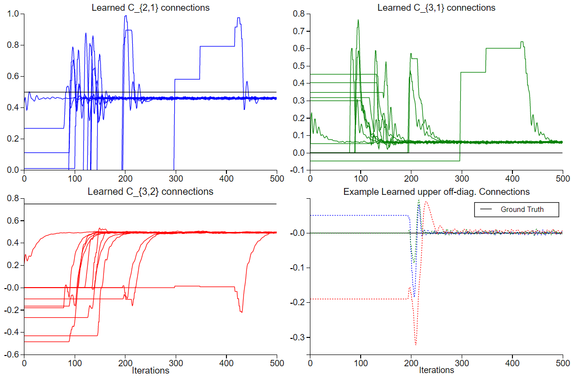
For the first example, we consider the chain network with connections
In 1, the connectivity estimation for the chain network is shown over iterations. In this case, we choose a regularization of . Each graph in the panels corresponds to a different random initialization of the connectivity matrix. At the beginning, the connections do not change because the sampler must learn an appropriate controller to bootstrap the procedure. Once the controller is estimated with sufficient accuracy, the ESS surpasses a threshold and the connectivity is updated via gradient ascent, hence the sudden jumps in the connections. After a few jumps, the learning procedure stabilizes and the connections are updated at each iteration. In most cases, it takes around 200-250 iterations to converge to the MAP solution.
The ESS after convergence of most examples increased from less than 1% to higher than 90% of total particles used. The mean state cost of the sampled process decreased in all cases from around 1000 to 68, meaning that the model found fits the data well.
Notice that the randomly initialized matrices converged all to the same values close to the ground truth. The connection is sufficiently weak and could be regarded as non existent since the other estimated connections dominate by an order of magnitude. The underestimation of the connection can be understood from the L1-penalty in the M-step to obtain sparse solutions. This regularization shrinks the connections by penalizing their absolute value. In turn, this shrinkage is compensated by an increase in the other incoming connection to node 3 to reduce the state cost, i.e. becomes non-zero. This hints to a strong regularization. To see the effect of strong regularization, we study the dependency of the solutions on the regularization strength .

For a fixed initialization of uncoupled nodes , the connections of the chain network are estimated using different values . The analysis shows–left panel of 2–that the ground truth connections (black dashed line) are consistently revealed across a wide range of -values. As expected, zero regularization gives small non-zero contributions in edges that would not be allowed, but still the ground truth connections are easy to differentiate. Hence, although the L1-regularization is not crucial in this example, we see that applying a small regularization helps shrinking the value of non existent connections towards zero, which improves the estimate of the network making it generalize better, as seen on the right panel of 2, where the mean validation error is shown.
To estimate the validation error we generate 1000 new time series using the ground truth connection and computed the mean negative log-likelihood or sate cost of the response obtained from each connectivity. This is a measure of how well our estimates fit the new data. We observe a decrease for weak regularization vis-�-vis the unregularized case and a strong increase in the validation error for increasing . From the minimum of this profile, we conclude that a weak regularization is beneficial, in this case using we obtain a solution pinpointing the ground truth to
Finally, we proceed with the estimation of the triangle network
to show that we obtain again the ground truth structure with a small regularization of . In 3, we observe a robust estimation against random initializations of the connectivity matrix and a clear distinction between correct and incorrect edges and directions. In this case, all estimated connections are around
Interestingly, in this case the overestimated connection is with the same order of magnitude as in the previous example. Again, we may vary to select its value by cross validation.

3.2 Identifying Networks with Fast Neuronal Activations
3.2.1 BOLD Sensitivity to Changes in the Connectivity Diminishes with Fast Neuronal Dynamics
The connectivity estimation above assumed that the temporal scale of the neuronal dynamics is of the order of a second. Here, we study the sensitivity of the BOLD response to changes in the connectivity as a function of . We consider 3 different time scales . The neuronal noise level is chosen such that the prior process has a standard deviation of 0.7%. The learning rate of APIS has to be adapted for the different values of , roughly with the relation . All other parameters of APIS are kept fixed.
Given the data generated by the chain network , the posterior statistics of the BOLD signal are estimated in two extreme cases using APIS; one case defines the structure and the other is close to the ground truth . The connectivity matrices are chosen such that the only difference to the ground truth are the connections into node 3,

In 4, we show the sensitivity of the BOLD response in node 3 when changing the connections from to . We appreciate two characteristics of the posterior BOLD response.
First, on the right panel, it is apparent that the variance of the signal has little sensitivity to the connectivity, with a change several orders of magnitude smaller than the change of the mean signal on the left. This suggests that–for small neuronal noise–the contribution of the variance to the identification of the connectivity is marginal and we can focus on the mean signal, which is equal to the BOLD signal of a deterministic system.
Second, on the left panel, for slow dynamics the amplitude of the mean signal change is larger than the observation noise level . However, already for the sensitivity decreases below the observation noise and it becomes an order of magnitude smaller for large . Hence, the faster the neuronal dynamics, the less sensible the BOLD response becomes to changes in the connectivity. The lack of sensitivity for faster time scales implies flat likelihood functions that contain no information to differentiate connectivity structures. Thus, should be sufficiently small such that the sensitivity is higher than the observation noise. This seems to be a fundamental problem to reconstruct connectivity.
One solution to this problem is more data, which effectively reduces the measurement noise. Another, option is to reconstruct with small and hope for the best. Thus, we study the grid search solutions obtained for different inverse time scales by the brute force search described before.
3.2.2 Connectivity Estimates Depend on the Assumed Neuronal Time Scale

We study now the connectivity estimates as a function of the inverse neuronal time scale . For each value of , we find the connections from 1000 different time series with the ground truth given by the chain network with the same parameters as before but . Figure 5 shows the mean and standard deviation of these estimates. Taking the amplitude of in 4 as a rough upper limit for the noise level that allows connectivity estimations, the analysis is performed with two noise levels, (on the top panels) and (on the bottom panels).
Upon examination of the top panels, we reinforce our expectation that with sufficient precision, the variance of the grid search solutions is small. Interestingly, the inverse time scale biases the connectivity estimates in a significant way. Nevertheless, it is possible to obtain in principle the correct connectivity if the time scale is jointly estimated because there is a clear minimum in the negative log-likelihood profile (red dot on the right panel).
On the contrary, with a noise level an order of magnitude higher, the identification of connections is problematic. Although the bias of the estimations is the same as above, the variance of the grid search solutions increases much faster with the inverse time scale because of the flat profiles of the neg. log-likelihood function. Thus, the grid search solutions spread across a wide range of values, making it difficult to pinpoint the connectivity. As a consequence, for identifying the correct connections will not be possible, even after learning the inverse time scale. This can be appreciated by the flat profile of the mean neg. log-likelihood at the grid search solutions.
Our analysis focuses on grid search solutions on the restricted connectivity space for simplicity. However, a similar analysis on the bidirectional connections results also in an extreme bias in the connectivity estimates due to the wrong time scale. This can be appreciated by inspecting the neg. log-likelihood landscape of a bidirectional connection with a mismatch in (not shown). As before, if the data is generated by a fast process but one assumes a slow process, the landscape is distorted and barely changes across different noise realizations and values of . The distorted landscape features a minimum around , although the data was generated using .

Finally, we study the variance of the connectivity estimates as a function of the observation noise . For this, data is generated with and the brute force search is performed without model mismatch. As expected from 5, the mean connectivity remains close to the ground truth values for all noise levels (not shown).
Figure 6 shows the standard deviation of the grid search connections . We observe that the noise level allowed for connectivity estimation depends on the inverse time scale of the neuronal dynamics. There are two effects here. First and most intuitive, the variance of the grid search connections increases with the observation noise. Notice the linear increase for large values in this log-log-graph. Second but more important, fast time scales in the neuronal signal exacerbate this increase at least an order of magnitude due to the insensitivity of the BOLD signal to changes in the connectivity. Notice how the dependency flattens by lowering the noise, first for , then for and finally for in the extreme high precision regime , where the standard deviation of the grid search solutions for and collapse. This shows that–even in this idealized case–to resolve connections when the neuronal time scale is around we require at most .
4 Discussion
In this paper we present a method to obtain point estimates of effective connectivity from fMRI time series. This method is based on the Expectation-Maximization algorithm with the E-step being performed by APIS on the same biologically plausible model used in DCM. We show that APIS-EM obtains robust estimations independent of random initializations of the connectivity matrix. In addition, we analyze the effect of the neuronal time scale on estimates of the effective connectivity. This analysis shows that if the underlying neuronal dynamics are fast, the connectivity estimates will be extremely biased if slow processes are assumed in the reconstruction. Hence, jointly estimating the neuronal time scale and the connectivity is important. However, due to the high insensitivity of the BOLD signal for faster neuronal dynamics, this becomes increasingly more demanding and requires higher quality data.
We conclude that robust reconstruction of the connectivity between ROIs including the directionality requires much higher precision in the data when assuming a realistic (fast) time scale for neuronal dynamics. In addition, if a slow time scale is assumed (as in [8, 9]) the inferred connectivity can be completely wrong if the generative neuronal process is fast.
The adaptive importance sampler APIS is an efficient tool to compute posterior estimates over the hidden processes. Importantly, the sampling step is easily parallelizable such that one can lower the computational burden involved in integrating the system of non-linear differential equations while having a large amount of samples to ensure reliable estimates.
Furthermore, APIS and its generalization based on PICE [kappen2015adaptive], are flexible frameworks that allow an easy adaptation of the M-step to learn the hemodynamic parameters by including noise in the hemodynamic degrees of freedom. Hence, instead of an -dimensional controller, APIS would learn a -dimensional controller. Although the computational burden increases in this case, we find empirically that the fully controlled version behaves more stable in terms of the effective sample size. Nevertheless, for simplicity we focused here on the reconstruction of the neural network and assumed the hemodynamic system is known. Hence, to maintain a lower computational cost, we chose the simplified, under-actuated setting.
Since the proposed scheme obtains robust estimates from randomly initialized connectivity matrices, it can be considered as a gradient-based exploratory procedure able to change the initial connectivity to find better fitting models. This addresses some of the concerns raised in [17]. Naturally, better initializations improve performance. A natural choice is the symmetric connectivity obtained from methods known to infer the right undirected network, for instance partial correlation or regularized inverse covariance.
Moreover, the addition of modulatory inputs or the consideration of more complex neuronal systems, e.g. firing rate models with non-linear activation functions, is straightforward. Furthermore, extensions of the proposed method to obtain Gaussian approximations of the posterior over all parameters similar to DCM can be worked out. This makes the combination of APIS and EM a flexible and efficient alternative to DCMs.
Finally, a word of caution. The bias in the connectivity estimates assuming the wrong time scale has significant consequences for the estimation of the hemodynamic parameters because the resulting BOLD signal is shifted roughly a second with respect to the ground truth. If both sets of parameters are jointly estimated, this shift will bias the hemodynamic parameters as well. On the contrary, fast neuronal dynamics make the delays being completely determined by the hemodynamics. This might lower the "interference" between delays caused by the neuronal time scale and the ones caused by the hemodynamics, possibly increasing identifiability of the hemodynamic system. Hence, it is important to clarify the temporal scale of the underlying processes, specially because this assumption has a major impact on the required quality of the data to obtain correct directed networks.
Acknowledgements
This work was supported by the European Commission through the FP7 Marie Curie Initial Training Network 289146, NETT: Neural Engineering Transformative Technologies.
Appendix: Validation of Grid Search on -Line
We validate the grid search approach by studying the neg. log-likelihood landscape on for two extreme cases with and without the correct inverse time scale. We show graphically that when there is a mismatch in , the bias caused by the restriction on the -line is small compared to the bias caused by the wrong time scale.

For the validation, data was generated using the chain network with and two different noise levels and . Figure 7 left panel shows the neg. log-likelihood on for estimated using the correct time scale. Although the high noise level ’washes out’ the -line (magenta), there is a clear direction along this line where the values are smallest. Perpendicular to this direction the value increases. Thus, minima lie in this case on the line. Due to the high noise level, the neg. log-likelihood along this line is flat. For lower noise levels, the valley becomes more and more narrow and the profile of the neg. log-likelihood on this line shows a clear minimum.
On the right panel of 7, we consider more precise data generated with but compute the neg. log-likelihood with a model mismatch in the time scale (). This distorts the landscape such that the low valued region around the -line transforms into an elliptic shaped valley with the minimum (dot #2) far away from the ground truth (dot #1). Notice how the major axis is parallel to the -line and, although the minimum does not lie exactly on the line, the error is small compare to the bias caused by the wrong time scale. Thus, restricting the search to the -line is a good approximation for the purpose of studying the grid search connections as a function of .
References
- [1] Michael Breakspear. Dynamic and stochastic models of neuroimaging data: A comment on lohmann et al. Neuroimage, 75:270–274, 2013.
- [2] Richard B Buxton, Eric C Wong, and Lawrence R Frank. Dynamics of blood flow and oxygenation changes during brain activation: the balloon model. Magnetic resonance in medicine, 39(6):855–864, 1998.
- [3] Arthur P Dempster, Nan M Laird, and Donald B Rubin. Maximum likelihood from incomplete data via the em algorithm. Journal of the royal statistical society. Series B (methodological), pages 1–38, 1977.
- [4] Karl Friston, Jean Daunizeau, and Klaas Enno Stephan. Model selection and gobbledygook: Response to lohmann et al. Neuroimage, 75:275–278, 2013.
- [5] Karl Friston, Rosalyn Moran, and Anil K Seth. Analysing connectivity with granger causality and dynamic causal modelling. Current opinion in neurobiology, 23(2):172–178, 2013.
- [6] Karl Friston, Klaas Stephan, Baojuan Li, and Jean Daunizeau. Generalised filtering. Mathematical Problems in Engineering, 2010, 2010.
- [7] Karl J Friston. Functional and effective connectivity in neuroimaging: a synthesis. Human brain mapping, 2(1-2):56–78, 1994.
- [8] Karl J Friston, Lee Harrison, and Will Penny. Dynamic causal modelling. Neuroimage, 19(4):1273–1302, 2003.
- [9] Karl J Friston, Baojuan Li, Jean Daunizeau, and Klaas E Stephan. Network discovery with dcm. Neuroimage, 56(3):1202–1221, 2011.
- [10] Karl J Friston, Andrea Mechelli, Robert Turner, and Cathy J Price. Nonlinear responses in fmri: the balloon model, volterra kernels, and other hemodynamics. NeuroImage, 12(4):466–477, 2000.
- [11] Igor Vladimirovich Girsanov. On transforming a certain class of stochastic processes by absolutely continuous substitution of measures. Theory of Probability & Its Applications, 5(3):285–301, 1960.
- [12] Rainer Goebel, Alard Roebroeck, Dae-Shik Kim, and Elia Formisano. Investigating directed cortical interactions in time-resolved fmri data using vector autoregressive modeling and granger causality mapping. Magnetic resonance imaging, 21(10):1251–1261, 2003.
- [13] Clive WJ Granger. Investigating causal relations by econometric models and cross-spectral methods. Econometrica: Journal of the Econometric Society, pages 424–438, 1969.
- [14] Pearl Judea. Causality: models, reasoning, and inference. Cambridge University Press. ISBN 0, 521(77362):8, 2000.
- [15] Hilbert J Kappen. Linear theory for control of nonlinear stochastic systems. Physical review letters, 95(20):200201, 2005.
- [16] Hilbert J Kappen, Vicenç Gómez, and Manfred Opper. Optimal control as a graphical model inference problem. Machine learning, 87(2):159–182, 2012.
- [17] Gabriele Lohmann, Kerstin Erfurth, Karsten Müller, and Robert Turner. Critical comments on dynamic causal modelling. Neuroimage, 59(3):2322–2329, 2012.
- [18] Joseph B Mandeville, John JA Marota, C Ayata, Greg Zaharchuk, Michael A Moskowitz, Bruce R Rosen, and Robert M Weisskoff. Evidence of a cerebrovascular postarteriole windkessel with delayed compliance. Journal of Cerebral Blood Flow & Metabolism, 19(6):679–689, 1999.
- [19] Radford M Neal and Geoffrey E Hinton. A view of the em algorithm that justifies incremental, sparse, and other variants. In Learning in graphical models, pages 355–368. Springer, 1998.
- [20] Rajan S Patel, F DuBois Bowman, and James K Rilling. A bayesian approach to determining connectivity of the human brain. Human brain mapping, 27(3):267–276, 2006.
- [21] Will Penny, Zoubin Ghahramani, and Karl Friston. Bilinear dynamical systems. Philosophical Transactions of the Royal Society of London B: Biological Sciences, 360(1457):983–993, 2005.
- [22] Joseph D Ramsey, Stephen José Hanson, Catherine Hanson, Yaroslav O Halchenko, Russell A Poldrack, and Clark Glymour. Six problems for causal inference from fmri. neuroimage, 49(2):1545–1558, 2010.
- [23] Hans-Christian Ruiz and Hilbert J Kappen. Particle smoothing for hidden diffusion processes: Adaptive path integral smoother. IEEE Transactions on Signal Processing, 65(12):3191–3203, 2017.
- [24] H.-Ch. Ruiz Euler and H.J. Kappen. Nonlinear deconvolution by sampling a biophysically plausible hemodynamic model. 2017.
- [25] Srikanth Ryali, Kaustubh Supekar, Tianwen Chen, and Vinod Menon. Multivariate dynamical systems models for estimating causal interactions in fmri. Neuroimage, 54(2):807–823, 2011.
- [26] Simo Särkkä. Bayesian filtering and smoothing, volume 3. Cambridge University Press, 2013.
- [27] Thomas B Schön, Adrian Wills, and Brett Ninness. System identification of nonlinear state-space models. Automatica, 47(1):39–49, 2011.
- [28] Stephen M Smith, Karla L Miller, Gholamreza Salimi-Khorshidi, Matthew Webster, Christian F Beckmann, Thomas E Nichols, Joseph D Ramsey, and Mark W Woolrich. Network modelling methods for fmri. Neuroimage, 54(2):875–891, 2011.
- [29] Klaas Enno Stephan, Lars Kasper, Lee M Harrison, Jean Daunizeau, Hanneke EM den Ouden, Michael Breakspear, and Karl J Friston. Nonlinear dynamic causal models for fmri. Neuroimage, 42(2):649–662, 2008.