Modelling and Analysing the Landing Gear System:
a Solution with Event-B/Rodin

Two modes are distinguished: a normal mode where the system is controlled digitally and its behaviour is correct if there is no anomaly detected in the system otherwise a permanent failure is observed; an emergency mode where the system is controlled analogically. Only the normal mode is in the scope of the case study (see page 1 of the requirement document).

Accordingly the boolean state output variable anomaly is used to denote that an anomaly has been detected or not (either $anomaly=TRUE$ or $anomaly=FALSE$). This variable is used to raise an anomaly and also to distinguish the two modes in the specification of properties and in the event guards.

One challenge of this case study is the construction of an abstract model which is as faithful as possible with the requirements. One of the properties of the landing system is at the same time doors cannot be closed and open. This is captured by the following predicate into the invariant of the building model:

$anomaly=FALSE⇒ran(door\_closed)∩ran(door\_open)=∅$

The digital part of the system controls the hydraulic devices according to the pilot orders and also to the mechanical devices positions (page 13 of the requirement document). This is achieved according to two specific action sequences: a landing action sequence and a retraction action sequence. An internal variable $order∈HSTATE$ is used to pass on the order issued by actioning the handle. The variable $order$ is an example of internal variable.

Moreover we have to take into account the requirements $R_{2}$ and $R_{3}$ (page 18 of the requirement document) which give the conditions of the orders (UP or DOWN) that can initiate the landing and retraction sequences and the conditions to enable them.

A thorough analysis of the two action sequences (outgoing sequence and retraction sequence) of the landing system helps us to capture the behaviour of the digital part. Even if they are nested each sequence is analysed precisely; it is made of a sequence of transition from state to state; each sequence is started as the effect of an action on the handle by the pilot. The remaining transitions in the sequence are mainly the orders from the digital part to the physical part, provided that some conditions described in the requirement document are established; therefore we are able to build a set of events (with conditions-actions) that describe as Event-B guarded events, the outgoing sequence and the retraction sequence.

In order to control perfectly the evolution of the outgoing sequence we use a variable $nextOGseq$ which indicates in the event guards the next step in the outgoing sequence. The variable is updated in the body of the events.

We now describe more precisely the outgoing sequence to illustrate our approach.

The outgoing sequence is defined at the page 14 of the requirement document. It starts with the order DOWN and is finished when the gears are extended and door closed. Between these events we have an interaction involving the digital part which issues the orders, the physical part which executes the orders and the sensors which provide the various states of the gears and doors. In Fig. 5 we depict the overall behaviour of the outgoing sequence, we can distinguish the main events and how they interact with the other components which are modelled: sensors and actuators. The labels of the transitions in the figure are the events that model the behaviour of the digital part with respect to the outgoing sequence. Note that the guards of the events depend on the current state of the transition system and on the state of the digital part (the sensors). In Fig. 5 we use the brackets to indicate the elements of the guards. The second sequence —retraction sequence— is modelled in the same way.

From the methodological point of view, we are still in the level 1 of Fig. 3; several horizontal refinements, depicted by the dashed arrows in the figure, are necessary to integrate gradually the variables and the related events.

The starting point is the state space obtained with the three categories of variables at the interface of the digital part and the fourth category of the internal variables. We define a family of events related to each category of the interface variables: monitoring events, control events, sensing events. Note that the construction of the abstract model is achieved gradually by incorporating the variables and the events.

The properties to be proved (requirements given in pages 18-19 of the requirement document) are formalised as first order predicates integrated into the invariant of the abstract model and proved along the horizontal refinement. Most of the normal mode requirements are safety properties. Requirement $R_{1}$ needs a specific treatment presented in the sequel.

• •

  Requirements $R_{21}$ and $R_{22}$.

  $R_{21}$	We can not observe a retraction sequence (consequence of the order $hUp$) if the handle is down. Using the enumerated set $HSTATE$ which permits only one value from two for the variable $order$,
  $order=hDown⇒ran(handle)≠\{hUp\}$

  $R_{22}$	In a similar way we cannot observe an outgoing sequence (consequence of the order $hDown$) if the handle is up.
  $order=hUp⇒ran(handle)≠\{hDown\}$

• •

  Requirements $R_{31}$ and $R_{32}$.

  $R_{31}$	The gears outgoing event occurs if doors are open locked
  $(extend\_EV=TRUE⇒ran(door\_open)=\{TRUE\})$

  $R_{32}$	The gears retraction event occurs if doors are open locked
  $(retract\_EV=TRUE⇒ran(door\_open)=\{TRUE\})$

• •

  Requirement $R_{41}$ and $R_{42}$.

  $R_{41}$	Opening and closing doors electro-valve are not stimulated simultaneously
  $¬(open\_EV=TRUE∧close\_EV=TRUE)$

  $R_{42}$	Outgoing and retraction gears electro-valve are not stimulated simultaneously
  $¬(extend\_EV=TRUE∧retract\_EV=TRUE)$

• •

  Requirement $R_{5}$.

  $R_{51}$	It is not possible to stimulate the manoeuvring EV (opening, closure, outgoing or retraction) without stimulating the general EV
  $((open\_EV=TRUE∨close\_EV=TRUE$
  $\penalty\ \penalty\ \penalty\ ∨extend\_EV=TRUE∨retract\_EV=TRUE)$
  $\penalty\ \penalty\ \penalty\ ⇒general\_EV=TRUE)$

The door behaviour is described at page 11 of the requirement document. It is first captured with a state automata; the transitions of the automata are then described as events. For this purpose we use a transition function $doorState∈DOOR\textrightarrow DSTATE$ where $DSTATE=\{ClosedLocked,ClosedUnlocked,OpenUnlocked\}$ is the enumerated set of the identified door states (see Fig. 7). The set $DOOR$ contains the three doors. The function $doorState$ is a total function; this captures the requirement that all the three doors are controlled via the state transition.

The starting transition of the door behaviour is enabled by the $open\_EV$ order³³ 3 In Fig. 7 the brackets indicate the event that contributes to enable the transition. given by the digital part. Therefore there is a synchronisation between the digital part and the doors. The remaining transitions are handled with events which are conveniently guarded in such a way that we have the correct ordering of the doors. Note that the three doors are simultaneously controlled by the orders issued by the digital part. We give below the description of the starting event (Door_openDoor_cl2cu).

event Door_openDoor_cl2cu /* Door’s Behaviour (for the three doors)    The first transition of the Door automata    enabled when the action open_EV is performed by the control system */ where $@g1\penalty\ \penalty\ open\_EV=TRUE$ // all doors EV are on $@g2\penalty\ \penalty\ ran(doorState)=\{notOpenLocked\}$ then $@a1doorState:=DOOR×\{notOpenNotLocked\}$ // door is being opened end

In the same way the transition starting from the open to close position is synchronised with the $close\_EV$ order given by the digital part. Therefore we have the complete interaction between between the orders from the digital part and the doors.

The gear behaviour is specified in the same way as the doors, see Fig. 8. A specific transition function is used: $gearState∈GEAR\textrightarrow GSTATE$ where $GSTATE=\{RetractedLocked,RetractedUnlocked,ExtendedUnlocked,ExtendedLocked\}$ is an enumerated set of gear states. The labels of the transition correspond to the events that model the behaviour of the gears. The set $GEAR$ contains the three gears.

The sensors behave like the observers of the door states and the gear states. When a door reaches the open state, then the related sensor events set the variable $door\_open$ to $TRUE$.

The related events in the specification are prefixed with sense_. The modelling of the sensors follows faithfully the requirement document; that is each sensor is made of three micro-sensors; each of them has its own state. We illustrate the modelling with the following event which deals with the extension of one micro-sensor⁴⁴ 4 identified by 1 of the front gear; the event sets the corresponding value in the interface variable ($gear\_extended$).

event sense1_FGE_OK // is sensor1 of Front Gear extended ? refines sense_gear any nge where $@noAno\penalty\ \penalty\ anomaly=FALSE$ $@g1\penalty\ \penalty\ gearState(FG)=LockE$ // the Front Gear is seen Locked Extended $@g2\penalty\ \penalty\ nge∈(TRIPLE×GEAR)\textrightarrow BOOL$ $@g3\penalty\ \penalty\ nge=gear\_extended<\!\!+\{(1\mapsto FG)\mapsto TRUE\}$ // update of the var then $@ea2\penalty\ \penalty\ gear\_extended:=nge$ // that is (1 $\mapsto$ FG) := TRUE end end

Note that a sensor can have an abnormal functioning. To simulate this anomaly on the sensor, the corresponding event could set the state of the gear to the wrong value. For this purpose, we define in our model such events, named likely sense1_FGE_KO, which set a wrong value.

Both modules have the same interface (input and output variables) inherited from the abstract model of the digital part.

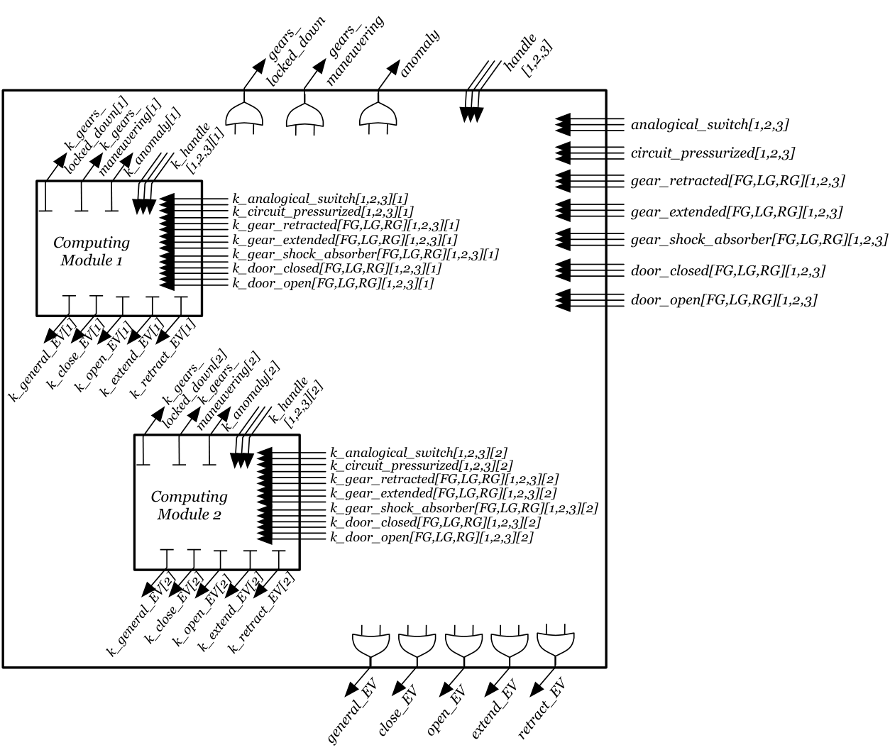
As far as the method is concerned, the principle of our solution is depicted in Fig. 11. Each interface variable of a module $k$ (where $k\in\{1,2\}$) is inherited from a variable (for instance $gear\_extended$) of the digital part of the abstract model and it is denoted by $k\_gear\_extended(k)$ where $(k)$ is an index. The prefix $k\_$ of the variable name enables us to keep the same name but to differentiate the abstract variable name and the refined one. An enumerated set $CompModule=\{1,2\}$ is used for the indexes. Therefore each interface variable of the computing modules is specified with the following shape, where the abstract variables are indexed.

$k\_handle∈CompModules\textrightarrow(TRIPLE\textrightarrow HSTATE)$ $k\_gear\_extended∈CompModule\textrightarrow((TRIPLE×GEAR)\textrightarrow BOOL)$ $k\_gear\_retracted∈CompModule\textrightarrow(TRIPLE×GEAR)\textrightarrow BOOL$ $k\_analogical\_switch∈CompModule\textrightarrow(TRIPLE\textrightarrow AnalSWSTATE)$ $k\_door\_closed∈CompModule\textrightarrow(TRIPLE×DOOR)\textrightarrow BOOL$ $k\_door\_open∈CompModule\textrightarrow(TRIPLE×DOOR)\textrightarrow BOOL$ $\cdots$ $k\_general\_EV∈CompModule\textrightarrow BOOL$ $k\_extend\_EV∈CompModules\textrightarrow BOOL$ $k\_close\_EV∈CompModule\textrightarrow BOOL$ $k\_open\_EV∈CompModule\textrightarrow BOOL$ $\cdots$

Notice, at this stage, the interface of the two modules are not linked with that of the abstract module. This is achieved via further refinement features: the binding between the variables and their k-indexed forms.

We have to specify that the inputs of the digital part (either from the cockpit or from the sensors) are the same ones for the computing modules. The principle adopted here is that the value of each input variable (for example $handle$) at the abstract level is pushed in the corresponding variable (for example $k\_handle$) of each computing module. As the inputs of the modules are (and should be) the same, an invariant is defined in each case of variable spawning in order to guarantee the correctness of the binding between the input variable of the digital part and the same input of the computing modules.

$handle∈ran(k\_handle)$ /* binding invariant */ $gear\_extended∈ran(k\_gear\_extended)$ /* binding invariant */

We use the following event pattern to spawn the variables at the interfaces of the computing modules.

event spawn_handleDown // spawn handleDown within the k CompModules where @g1 $ran(handle)=\{hDown\}$ then @a1 $k\_handle:=\{1\mapsto(TRIPLE×(ran(handle))),$ $\penalty\ \penalty\ \penalty\ \penalty\ \penalty\ \penalty\ \penalty\ \penalty\ \penalty\ \penalty\ \penalty\ \penalty\ \penalty\ \penalty\ 2\mapsto(TRIPLE×(ran(handle)))\}$ end

Consequently one identified specification rule is that a new event is introduced along with each new k-indexed variable. This event should copy the variable at high level (the digital part) into the indexed variables at the low level. This specification rule is reusable in all such cases where variables from a module should be buried inside submodules.

Furthermore, the existing events, which guards or actions involve spawned variables, should be refined by extending their guards and actions in order to satisfy the binding between the variables and the associated k-indexed variables.

As far as the input from the sensors are concerned, specific treatment is needed in order to take account of the separate behaviours of the three micro-sensors that can send different values event wrong values. For this purpose, if we consider each (front, left, right) door or gear, two events are needed to specify the impact of the micro-sensor behaviour on the k-indexed input variables of the computing modules; one event gives the right value of the micro-sensor, whereas the other event gives the wrong value.

One noticeable feature in this case is that when we have a nondeterministic event of abstract level (as for the value of the sensors), then in the refinement the event should be refined (not extended). This is a second identified specification rule.

As an example, we consider the sensor 2 from the three sensors that sense if the left door is open ($LDO$), hence the event names $sense2\_LDO\_OK$, $sense2\_LDO\_KO$.

event event sense2_LDO_OK // seonsor2 of LDoor extends sense2_LDO_OK any nkdo where $@noano\penalty\ \penalty\ ∀kk.(kk∈CompModules⇒(k\_anomaly(kk)=FALSE))$ $@dnkge\penalty\ \penalty\ nkdo∈CompModules\textrightarrow((TRIPLE×DOOR)\textrightarrow BOOL)$ $@nge\penalty\ \penalty\ nkdo\penalty\ =CompModules×\{door\_open<+\{(2\mapsto LD)\mapsto TRUE\}\}$ then $@ea1k\_door\_open:=nkdo$ end

event event sense2_LDO_KO // sensor2 of FDoor (simulating malfunctioning) extends sense2_LDO_KO any nkdo where $@noano\penalty\ \penalty\ ∀kk.(kk∈CompModules⇒(k\_anomaly(kk)=FALSE))$ $@dnkge\penalty\ \penalty\ nkdo∈CompModules\textrightarrow((TRIPLE×DOOR)\textrightarrow BOOL)$ $@nge\penalty\ \penalty\ nkdo=CompModules×\{door\_open<+\{(2\mapsto LD)\mapsto FALSE\}\}$ then $@ea1\penalty\ \penalty\ k\_door\_open:=nkdo$ end

The specification principle is as follows. As presented in the requirement and depicted in Fig. 11, the k-indexed output variables (for example $k\_extend\_EV(1)$ and $k\_extend\_EV(2)$) are merged using a logical OR to set the corresponding variable (for example $extend\_EV$) at the output of the digital part. Therefore the event that sets the variable should be guarded by the availability of the merged value. As explained before, a binding invariant should be provided for each variable and the related k-indexed variable.

$k\_extend\_EV∈CompModules\textrightarrow BOOL$ $extend\_EV∈ran(k\_extend\_EV)$ /* binding invariant */

The merging is illustrated with the following event $merge\_stmlt\_gear\_outgoing$, which updates the output variable $extend\_EV$. Only the guard should be extended in the refinement since the abstract event already has the right substitution to set the variable.

event merge_stmlt_gear_outgoing /* MERGING the result of the k module to stimulate the gear_outgoing ** action 3 ** of outgoing sequence */ extends stmlt_gear_outgoing any kk where $@gkk\penalty\ \penalty\ kk∈CompModules$ $@theOR\penalty\ \penalty\ k\_extend\_EV(kk)=TRUE$ /* OR : one of them is TRUE */ end

References

- [1] Abrial, J.R.: Modeling in Event-B - System and Software Engineering. Cambridge University Press (2010)
- [2] Butler, M., Yadav, D.: An Incremental Development of the Mondex System in Event-B. Formal Asp. Comput. 20(1) (2008) 61–77
- [3] Lanoix, A.: Event-B Specification of a Situated Multi-Agent System: Study of a Platoon of Vehicles. In: 2nd IFIP/IEEE International Symposium on Theoretical Aspects of Software Engineering (TASE 2008), France (June 2008) 8 pages
- [4] Damchoom, K., Butler, M.J.: Applying Event and Machine Decomposition to a Flash-Based Filestore in Event-B. In Oliveira, M.V.M., Woodcock, J., eds.: SBMF. Volume 5902 of Lecture Notes in Computer Science., Springer (2009) 134–152
- [5] Cansell, D., Méry, D., Proch, C.: System-on-chip design by proof-based refinement. STTT 11(3) (2009) 217–238
- [6] Fathabadi, A.S., Rezazadeh, A., Butler, M.: Applying Atomicity and Model Decomposition to a Space Craft System in Event-B. In: NASA Formal Methods. (2011) 328–342
- [7] Méry, D., Singh, N.K.: Formal Specification of Medical Systems by Proof-Based Refinement. ACM Trans. Embedded Comput. Syst. 12(1) (2013) 15
- [8] Damchoom, K., Butler, M.J., Abrial, J.R.: Modelling and Proof of a Tree-Structured File System in Event-B and Rodin. In Liu, S., Maibaum, T.S.E., Araki, K., eds.: ICFEM. Volume 5256 of Lecture Notes in Computer Science., Springer (2008) 25–44
- [9] Lamport, L.: Time, Clocks, and the Ordering of Events in a Distributed System. Commun. ACM 21(7) (1978) 558–565
- [10] Abrial, J.R., Hallerstede, S.: Refinement, Decomposition, and Instantiation of Discrete Models: Application to Event-B. Fundam. Inform. 77(1-2) (2007) 1–28
- [11] Butler, M.: Decomposition Structures for Event-B. In Leuschel, M., Wehrheim, H., eds.: IFM. Volume 5423 of Lecture Notes in Computer Science., Springer (2009) 20–38
- [12] Silva, R., Butler, M.: Shared Event Composition/Decomposition in Event-B. In Aichernig, B.K., de Boer, F.S., Bonsangue, M.M., eds.: FMCO. Volume 6957 of Lecture Notes in Computer Science., Springer (2010) 122–141
- [13] Back, R.J.: Software Construction by Stepwise Feature Introduction. In Bert, D., Bowen, J.P., Henson, M.C., Robinson, K., eds.: ZB. Volume 2272 of Lecture Notes in Computer Science., Springer (2002) 162–183
- [14] Parnas, D.L., Madey, J.: Functional Documents for Computer Systems. Sci. Comput. Program. 25(1) (1995) 41–61