An Assertion-Based Program Logic
for Probabilistic
ProgramsThanks: This is the full version of the paper.
Abstract
Research on deductive verification of probabilistic programs has considered expectation-based logics, where pre- and post-conditions are real-valued functions on states, and assertion-based logics, where pre- and post-conditions are boolean predicates on state distributions. Both approaches have developed over nearly four decades, but they have different standings today. Expectation-based systems have managed to formalize many sophisticated case studies, while assertion-based systems today have more limited expressivity and have targeted simpler examples.
We present Ellora, a sound and relatively complete assertion-based program logic, and demonstrate its expressivity by verifying several classical examples of randomized algorithms using an implementation in the EasyCrypt proof assistant. Ellora features new proof rules for loops and adversarial code, and supports richer assertions than existing program logics. We also show that Ellora allows convenient reasoning about complex probabilistic concepts by developing a new program logic for probabilistic independence and distribution law, and then smoothly embedding it into Ellora. Our work demonstrates that the assertion-based approach is not fundamentally limited and suggests that some notions are potentially easier to reason about in assertion-based systems.
1 Introduction
The most mature systems for deductive verification of randomized algorithms are expectation-based techniques; seminal examples include PPDL [25] and pGCL [31]. These approaches reason about expectations, functions from states to real numbers,11 1 Treating a program as a function from input states to output distributions , the expected value of on is an expectation. propagating them backwards through a program until they are transformed into a mathematical function of the input. Expectation-based systems are both theoretically elegant [21, 13, 32, 20] and practically useful; implementations have verified numerous randomized algorithms [16, 18]. However, properties involving multiple probabilities or expected values can be cumbersome to verify—each expectation must be analyzed separately.
An alternative approach envisioned by Ramshaw [34] is to work with predicates over distributions. A direct comparison with expectation-based techniques is difficult, as the approaches are quite different. In broad strokes, assertion-based systems can verify richer properties in one shot and have specifications that are arguably more intuitive, especially for reasoning about loops, while expectation-based approaches can transform expectations mechanically and can reason about non-determinism. However, the comparison is not very meaningful for an even simpler reason: existing assertion-based systems such as [7, 15, 35] are not as well developed as their expectation-based counterparts.
- Restrictive assertions.
-
Existing probabilistic program logics do not support reasoning about expected values, only probabilities. As a result, many properties about average-case behavior are not even expressible.
- Inconvenient reasoning for loops.
-
The Hoare logic rule for deterministic loops does not directly generalize to probabilistic programs. Existing assertion-based systems either forbid loops, or impose complex semantic side conditions to control which assertions can be used as loop invariants. Such side conditions are restrictive and difficult to establish.
- No support for external or adversarial code.
-
A strength of expectation-based techniques is reasoning about programs combining probabilities and non-determinism. In contrast, Morgan and McIver [27] argue that assertion-based techniques cannot support compositional reasoning for such a combination. For many applications, including cryptography, we would still like to reason about a commonly-encountered special case: programs using external or adversarial code. Many security properties in cryptography boil down to analyzing such programs, but existing program logics do not support adversarial code.
- Few concrete implementations.
-
There are by now several independent implementations of expectation-based techniques, capable of verifying interesting probabilistic programs. In contrast, there are only scattered implementations of probabilistic program logics.
These limitations raise two points. Compared to expectation-based approaches:
- 1.
Can assertion-based approaches achieve similar expressivity?
- 2.
Are there situations where assertion-based approaches are more suitable?
In this paper, we give positive evidence for both of these points.22 2 Note that we do not give mathematically precise formulations of these points; as we are interested in the practical verification of probabilistic programs, a purely theoretical answer would not address our concerns. Towards the first point, we give a new assertion-based logic Ellora for probabilistic programs, overcoming limitations in existing probabilistic program logics. Ellora supports a rich set of assertions that can express concepts like expected values and probabilistic independence, and novel proof rules for verifying loops and adversarial code. We prove that Ellora is sound and relatively complete.
Towards the second point, we evaluate Ellora in two ways. First, we define a new logic for proving probabilistic independence and distribution law properties—which are difficult to capture with expectation-based approaches—and then embed it into Ellora. This sub-logic is more narrowly focused than Ellora, but supports more concise reasoning for the target assertions. Our embedding demonstrates that the assertion-based approach can be flexibly integrated with intuitive, special-purpose reasoning principles. To further support this claim, we also provide an embedding of the Union Bound logic, a program logic for reasoning about accuracy bounds [4]. Then, we develop a full-featured implementation of Ellora in the EasyCrypt theorem prover and exercise the logic by mechanically verifying a series of complex randomized algorithms. Our results suggest that the assertion-based approach can indeed be practically viable.
Abstract logic.
To ease the presentation, we present Ellora in two stages. First, we consider an abstract version of the logic where assertions are general predicates over distributions, with no compact syntax. Our abstract logic makes two contributions: reasoning for loops, and for adversarial code.
Reasoning about Loops.
Proving a property of a probabilistic loop typically requires establishing a loop invariant, but the class of loop invariants that can be soundly used depends on the termination behavior—stronger termination assumptions allows richer loop invariants. We identify three classes of assertions that can be used for reasoning about probabilistic loops, and provide a proof rule for each one:
- •
arbitrary assertions for certainly terminating loops, i.e. loops that terminate in a finite amount of iterations;
- •
topologically closed assertions for almost surely terminating loops, i.e. loops terminating with probability ;
- •
downwards closed assertions for arbitrary loops.
The definition of topologically closed assertion is reminiscent of Ramshaw [34]; the stronger notion of downwards closed assertion appears to be new.
Besides broadening the class of loops that can be analyzed, our rules often enable simpler proofs. For instance, if the loop is certainly terminating, then there is no need to prove semantic side-conditions. Likewise, there is no need to consider the termination behavior of the loop when the invariant is downwards and topologically closed. For example, in many applications in cryptography, the target property is that a “bad” event has low probability: . In our framework this assertion is downwards and topologically closed, so it can be a loop invariant regardless of the termination behavior.
Reasoning about Adversaries.
Existing assertion-based logics cannot reason about probabilistic programs with adversarial code. Adversaries are special probabilistic procedures consisting of an interface listing the concrete procedures that an adversary can call (oracles), along with restrictions like how many calls an adversary may make. Adversaries are useful in cryptography, where security notions are described using experiments in which adversaries interact with a challenger, and in game theory and mechanism design, where adversaries can represent strategic agents. Adversaries can also model inputs to online algorithms.
We provide proof rules for reasoning about adversary calls. Our rules are significantly more general than previously considered rules for reasoning about adversaries. For instance, the rule for adversary used by [4] is restricted to adversaries that cannot make oracle calls.
Metatheory.
We show soundness and relative completeness of the core abstract logic, with mechanized proofs in the Coq proof assistant.33 3 The formalization is available at https://github.com/strub/xhl.
Concrete logic.
While the abstract logic is conceptually clean, it is inconvenient for practical formal verification—the assertions are too general and the rules involve semantic side-conditions. To address these issues, we flesh out a concrete version of Ellora. Assertions are described by a grammar modeling a two-level assertion language. The first level contains state predicates—deterministic assertions about a single memory—while the second layer contains probabilistic predicates constructed from probabilities and expected values over discrete distributions. While the concrete assertions are theoretically less expressive than their counterparts in the abstract logic, they can already encode common properties and notions from existing proofs, like probabilities, expected values, distribution laws and probabilistic independence. Our assertions can express theorems from probability theory, enabling sophisticated reasoning about probabilistic concepts.
Furthermore, we leverage the concrete syntax to simplify verification.
- •
We develop an automated procedure for generating pre-conditions of non-looping commands, inspired by expectation-based systems.
- •
We give syntactic conditions for the closedness and termination properties required for soundness of the loop rules.
Implementation and case studies.
We implement Ellora on top of EasyCrypt, a general-purpose proof assistant for reasoning about probabilistic programs, and we mechanically verify a diverse collection of examples including textbook algorithms and a randomized routing procedure. We develop an EasyCrypt formalization of probability theory from the ground up, including tools like concentration bounds (e.g., the Chernoff bound), Markov’s inequality, and theorems about probabilistic independence.
Embeddings.
We propose a simple program logic for proving probabilistic independence. This logic is designed to reason about independence in a lightweight way, as is common in paper proofs. We prove that the logic can be embedded into Ellora, and is therefore sound. Furthermore, we prove an embedding of the Union Bound logic [4].
2 Mathematical Preliminaries
As is standard, we will model randomized computations using sub-distributions.
Definition 1.
A sub-distribution over a set is defined by a mass function that gives the probability of the unitary events . This mass function must be s.t. is well-defined and . In particular, the support is discrete.44 4 We work with discrete distributions to keep measure-theoretic technicalities to a minimum, though we do not see obstacles to generalizing to the continuous setting. The name “sub-distribution” emphasizes that the total probability may be strictly less than . When the weight is equal to , we call a distribution. We let denote the set of sub-distributions over . The probability of an event w.r.t. a sub-distribution , written , is defined as .
Simple examples of sub-distributions include the null sub-distribution , which maps each element of the underlying space to ; and the Dirac distribution centered on , written , which maps to and all other elements to . The following standard construction gives a monadic structure to sub-distributions.
Definition 2.
Let and . Then is defined by
We use notation reminiscent of expected values, as the definition is quite similar.
We will need two constructions to model branching statements.
Definition 3.
Let such that . Then is the sub-distribution such that for every .
Definition 4.
Let and . Then the restriction of to is the sub-distribution such that if and 0 otherwise.
Sub-distributions are partially ordered under the pointwise order.
Definition 5.
Let . We say if for every , and we say if for every .
We use the following lemma when reasoning about the semantics of loops.
Lemma 1
If and , then and .
Sub-distributions are stable under pointwise-limits.
Definition 6.
A sequence sub-distributions converges if for every , the sequence of real numbers converges. The limit sub-distribution is defined as
for every . We write for .
Lemma 2
Let be a convergent sequence of sub-distributions. Then for any event , we have:
Any bounded increasing real sequence has a limit; the same is true of sub-distributions.
Lemma 3
Let be an increasing sequence of sub-distributions. Then, this sequence converges to and for every . In particular, for any event , we have for every .
3 Programs and Assertions
Now, we introduce our core programming language and its denotational semantics.
Programs.
We base our development on pWhile, a strongly-typed imperative language with deterministic assignments, probabilistic assignments, conditionals, loops, and an statement which halts the computation with no result. Probabilistic assignments assign a value sampled from a distribution to a program variable . The syntax of statements is defined by the grammar:
where , , and range over typed variables in , expressions in and distribution expressions in respectively. The set of well-typed expressions is defined inductively from and a set of function symbols, while the set of well-typed distribution expressions is defined by combining a set of distribution symbols with expressions in . Programs may call a set of internal procedures as well as a set of external procedures. We assume that we have code for internal procedures but not for external procedures—we only know indirect information, like which internal procedures they may call. Borrowing a convention from cryptography, we call internal procedures oracles and external procedures adversaries.
Semantics.
The denotational semantics of programs is adapted from the seminal work of [24] and interprets programs as sub-distribution transformers. We view states as type-preserving mappings from variables to values; we write for the set of states and for the set of probabilistic states. For each procedure name , we assume a set of local variables s.t. are pairwise disjoint. The other variables are global variables.
To define the interpretation of expressions and distribution expressions, we let denote the interpretation of expression with respect to state , and denote the interpretation of expression with respect to an initial sub-distribution over states defined by the clause . Likewise, we define the semantics of commands in two stages: first interpreted in a single input memory, then interpreted in an input sub-distribution over memories.
Definition 7.
The semantics of commands are given in Fig. 1.
- •
The semantics of a statement in initial state is a sub-distribution over states.
- •
The (lifted) semantics of a statement in initial sub-distribution over states is a sub-distribution over states.
We briefly comment on loops. The semantics of a loop is defined as the limit of its lower approximations, where the -th lower approximation of is , where is shorthand for and is the -fold composition . Since the sequence is increasing, the limit is well-defined by Lemma 3. In contrast, the -th approximation of defined by may not converge, since they are not necessarily increasing. However, in the special case where the output distribution has weight , the -th lower approximations and the -th approximations have the same limit.
Lemma 4
If the sub-distribution has weight , then the limit of is defined and
This follows by Lemma 1, since lower approximations are below approximations so the limit of their weights (and the weight of their limit) is . It will be useful to identify programs that terminate with probability .
Definition 8 (Lossless).
A statement is lossless if for every sub-distribution , , where is the total probability of . Programs that are not lossless are called lossy.
Informally, a program is lossless if all probabilistic assignments sample from full distributions rather than sub-distributions, there are no instructions, and the program is almost surely terminating, i.e. infinite traces have probability zero. Note that if we restrict the language to sample from full distributions, then losslessness coincides with almost sure termination.
Another important class of loops are loops with a uniform upper bound on the number of iterations. Formally, we say that a loop is certainly terminating if there exists such that for every sub-distribution , we have . Note that certain termination of a loop does not entail losslessness—the output distribution of the loop may not have weight , for instance, if the loop samples from a sub-distribution or if the loop aborts with positive probability.
Semantics of Procedure Calls and Adversaries.
The semantics of internal procedure calls is straightforward. Associated to each procedure name , we assume a designated input variable , a piece of code that executes the function call, and a result expression . A function call is then equivalent to . Procedures are subject to well-formedness criteria: procedures should only use local variables in their scope and after initializing them, and should not perform recursive calls.
External procedure calls, also known as adversary calls, are a bit more involved. Each name is parametrized by a set of internal procedures which the adversary may call, a designated input variable , a (unspecified) piece of code that executes the function call, and a result expression . We assume that adversarial code can only access its local variables in and can only make calls to procedures in . It is possible to impose more restrictions on adversaries—say, that they are lossless—but for simplicity we do not impose additional assumptions on adversaries here.
4 Proof System
In this section we introduce a program logic for proving properties of probabilistic programs. The logic is abstract—assertions are arbitrary predicates on sub-distributions—but the meta-theoretic properties are clearest in this setting. In the following section, we will give a concrete version suitable for practical use.
Assertions and Closedness Conditions.
We use predicates on state distribution.
Definition 9 (Assertions).
The set of assertions is defined as . We write for .
Usual set operations are lifted to assertions using their logical counterparts, e.g., and . Our program logic uses a few additional constructions. Given a predicate over states, we define
where is the set of all states with non-zero probability under . Intuitively, holds deterministically on all states that we may sample from the distribution. To reason about branching commands, given two assertions and , we let
This assertion means that the sub-distribution is the sum of two sub-distributions such that holds on the first piece and holds on the second piece.
Given an assertion and an event , we let This assertion holds exactly when is true on the portion of the sub-distribution satisfying . Finally, given an assertion and a function from to , we define Intuitively, is true in a sub-distribution exactly when holds on .
Now, we can define the closedness properties of assertions. These properties will be critical to our rules for loops.
Definition 10 (Closedness properties).
A family of assertions is:
- •
-closed if for every increasing sequence of sub-distributions such that for all then ;
- •
-closed if for every converging sequence of sub-distributions such that for all then ;
- •
-closed if it is -closed and downward closed, that is for every sub-distributions , implies .
When is constant and equal to , we say that is -/-/-closed.
Note that -closedness implies -closedness, but the converse does not hold. Moreover, -closed, -closed and -closed assertions are closed under arbitrary intersections and finite unions, or in logical terms under finite boolean combinations, universal quantification over arbitrary sets and existential quantification over finite sets.
Finally, we introduce the necessary machinery for the frame rule. The set of modified variables of a statement consists of all the variables on the left of a deterministic or probabilistic assignment. In this setting, we say that an assertion is separated from a set of variables , written , if for any distributions , s.t. and where for a set of variables , the restricted sub-distribution is
where and restrict and to the variables in .
Intuitively, an assertion is separated from a set of variables if every two sub-distributions that agree on the variables outside either both satisfy the assertion, or both refute the assertion.
Judgments and Proof Rules.
Judgments are of the form , where the assertions and are drawn from .
Definition 11.
A judgment is valid, written , if for every interpretation of adversarial procedures and every probabilistic state such that .
Figure 2 describes the structural and basic rules of the proof system. Validity of judgments is preserved under standard structural rules, like the rule of consequence [Conseq]. As usual, the rule of consequence allows to weaken the post-condition and to strengthen the post-condition; in our system, this rule serves as the interface between the program logic and mathematical theorems from probability theory. The [Exists] rule is helpful to deal with existentially quantified pre-conditions.
The rules for , assignments, random samplings and sequences are all straightforward. The rule for requires to hold after execution; this assertion uniquely characterizes the resulting null sub-distribution. The rules for assignments and random samplings are semantical.
The rule [Cond] for conditionals requires that the post-condition must be of the form ; this reflects the semantics of conditionals, which splits the initial probabilistic state depending on the guard, runs both branches, and recombines the resulting two probabilistic states.
The next two rules ([Split] and [Frame]) are useful for local reasoning. The [Split] rule reflects the additivity of the semantics and combines the pre- and post-conditions using the operator. The [Frame] rule asserts that lossless statements preserve assertions that are not influenced by modified variables.
The rule [Call] for internal procedures is as expected, replacing the procedure call with its definition.
Figure 3 presents the rules for loops. We consider four rules specialized to the termination behavior. The [While] rule is the most general rule, as it deals with arbitrary loops. For simplicity, we explain the rule in the special case where the family of assertions is constant, i.e. we have and . Informally, the is the loop invariant and is an auxiliary assertion used to prove the invariant. We require that is -closed, since the semantics of a loop is defined as the limit of its lower approximations. Moreover, the first premise ensures that starting from , one guarded iteration of the loop establishes ; the second premise ensures that restricting to a probabilistic state satisfying yields a probabilistic state satisfying . It is possible to give an alternative formulation where the second premise is substituted by the logical constraint . As usual, the post-condition of the loop is the conjunction of the invariant with the negation of the guard (more precisely in our setting, that the guard has probability 0).
The [While-AST] rule deals with lossless loops. For simplicity, we explain the rule in the special case where the family of assertions is constant, i.e. we have . In this case, we know that lower approximations and approximations have the same limit, so we can directly prove an invariant that holds after one guarded iteration of the loop. On the other hand, we must now require that the satisfies the stronger property of -closedness.
The [While-D] rule handles arbitrary loops with a -closed invariant; intuitively, restricting a sub-distribution that satisfies a downwards closed assertion yields a sub-distribution which also satisfies .
The [While-CT] rule deals with certainly terminating loops. In this case, there is no requirement on the assertions.
We briefly compare the rules from a verification perspective. If the assertion is -closed, then the rule [While-D] is easier to use, since there is no need to prove any termination requirement. Alternatively, if we can prove certain termination of the loop, then the rule [While-CT] is the best to use since it does not impose any condition on assertions. When the loop is lossless, there is no need to introduce an auxiliary assertion , which simplifies the proof goal. Note however that it might still be beneficial to use the [While] rule, even for lossless loops, because of the weaker requirement that the invariant is -closed rather than -closed.
Finally, Fig. 4 gives the adversary rule for general adversaries. It is highly similar to the general rule [While-D] for loops since the adversary may make an arbitrary sequence of calls to the oracles in and may not be lossless. Intuitively, plays the role of the invariant: it must be -closed and it must be preserved by every oracle call with arbitrary arguments. If this holds, then is also preserved by the adversary call. Some framing conditions are required, similar to the ones of the [Frame] rule: the invariant must not be influenced by the state writable by the external procedures.
It is possible to give other variants of the adversary rule with more general invariants by restricting the adversary, e.g., requiring losslessness or bounding the number of calls the external procedure can make to oracles, leading to rules akin to the almost surely terminating and certainly terminating loop rules, respectively.
Soundness and Relative Completeness.
Our proof system is sound and relatively complete with respect to the semantics; these proofs have also been formalized in the Coq proof assistant.
Theorem 4.1 (Soundness)
Every judgment provable using the rules of our logic is valid.
Completeness of the logic follows from the next lemma, whose proof makes an essential use of the [While] rule. In the sequel, we use to denote the characteristic function of a probabilistic state , an assertion stating that the current state is equal to .
Lemma 5
For every probabilistic state , the following judgment is provable using the rule of the logic:
Proof.
By induction on the structure of .
- •
, , and are trivial;
- •
, we have to prove
We apply the [Seq] rule with premises can be directly proved using the induction hypothesis;
- •
, we have to prove
We apply the [Conseq] rule to be able to apply the the [Cond] rule with and Both premises can be proved by an application of the [Conseq] rule followed by the application of the induction hypothesis.
- •
, we have to prove
We first apply the [While] rule with and
For the first premise we apply the same process as for the conditional case: we apply the [Conseq] and [Cond] rules and we conclude using the induction hypothesis (and the [Skip] rule). For the second premise we follow the same process but we conclude using the [Abort] rule instead of the induction hypothesis. Finally we conclude since . ∎
The abstract logic is also relatively complete. This property will be less important for our purposes, but it serves as a basic sanity check.
Theorem 4.2 (Relative completeness)
Every valid judgment is derivable.
Proof.
Consider a valid judgment . Let be a probabilistic state such that . By the above proposition, . Using the validity of the judgment and [Conseq], we have . Using the [Exists] and [Conseq] rules, we conclude as required. ∎
The side-conditions in the loop rules (e.g., // and the weight conditions) are difficult to prove, since they are semantic properties. Next, we present a concrete version of the logic with give easy-to-check, syntactic sufficient conditions.
5 A Concrete Program Logic
To give a more practical version of the logic, we begin by setting a concrete syntax for assertions
Assertions.
We use a two-level assertion language, presented in Fig. 5. A probabilistic assertion is a formula built from comparison of probabilistic expressions, using first-order quantifiers and connectives, and the special connective . A probabilistic expression can be a logical variable , an operator applied to probabilistic expressions (constants are -ary operators), or the expectation of a state expression . A state expression is either a program variable , the characteristic function of a state assertion , an operator applied to state expressions , or the expectation of state expression in a given distribution . Finally, a state assertion is a first-order formula over program variables. Note that the set of operators is left unspecified but we assume that all the expressions in and can be encoded by operators.
| (S-expr.) | ||||
| (S-assn.) | ||||
| (P-expr.) | ||||
| (P-assn.) | ||||
| (Ops.) |
The interpretation of the concrete syntax is as expected. The interpretation of probabilistic assertions is relative to a valuation which maps logical variables to values, and is an element of . The definition of the interpretation is straightforward; the only interesting case is which is defined by , where is the interpretation of the state expression in the memory and valuation . The interpretation of state expressions is a mapping from memories to values, which can be lifted to a mapping from distributions over memories to distributions over values. The definition of the interpretation is straightforward; the most interesting case is for expectation . We present the full interpretations in the supplemental materials.
Many standard concepts from probability theory have a natural representation in our syntax. For example:
- •
the probability that holds in some probabilistic state is represented by the probabilistic expression ;
- •
probabilistic independence of state expressions , …, is modeled by the probabilistic assertion , defined by the clause55 5 The term is necessary since we work with sub-distributions.
- •
the fact that a distribution is proper is modeled by the probabilistic assertion ;
- •
a state expression distributed according to a law is modeled by the probabilistic assertion
The inner expectation computes the probability that drawn from is equal to a fixed ; the outer expectation weights the inner probability by the probability of each value of .
We can easily define operator from the previous section in our new syntax: .
Syntactic Proof Rules.
Now that we have a concrete syntax for assertions, we can give syntactic versions of many of the existing proof rules. Such proof rules are often easier to use since they avoid reasoning about the semantics of commands and assertions. We tackle the non-looping rules first, beginning with the following syntactic rules for assignment and sampling:
The rule for assignment is the usual rule from Hoare logic, replacing the program variable by its corresponding expression in the pre-condition. The replacement is done recursively on the probabilistic assertion ; for instance for expectations, it is defined by where is the syntactic substitution.
The rule for sampling uses probabilistic substitution operator , which replaces all occurrences of in by a new integration variable and records that is drawn from ; the operator is defined in Fig. 6.
for .
Next, we turn to the loop rule. The side-conditions from Fig. 3 are purely semantic, while in practice it is more convenient to use a sufficient condition in the Hoare logic. We give sufficient conditions for ensuring certain and almost-sure termination in Fig. 7; is an integer-valued expression. The first side-condition shows certain termination given a strictly decreasing variant that is bounded below, similar to how a decreasing variant shows termination for deterministic programs. The second side-condition shows almost-sure termination given a probabilistic variant , which must be bounded both above and below. While may increase with some probability, it must decrease with strictly positive probability. This condition was previously considered by [14] for probabilistic transition systems and also used in expectation-based approaches [30, 17]. Our framework can also support more refined conditions (e.g., based on super-martingales [8, 28]), but the condition already suffices for most randomized algorithms.
While -closedness is a semantic condition (cf. Definition 10), there are simple syntactic conditions to guarantee it. For instance, assertions that carry a non-strict comparison between two bounded probabilistic expressions are -closed; the assertion stating probabilistic independence of a set of expressions is -closed.
Precondition Calculus.
With a concrete syntax for assertions, we are also able to incorporate syntactic reasoning principles. One classic tool is Morgan and McIver’s greatest pre-expectation, which we take as inspiration for a pre-condition calculus for the loop-free fragment of Ellora. Given an assertion and a loop-free statement , we mechanically construct an assertion that is the pre-condition of that implies as a post-condition. The basic idea is to replace each expectation expression inside by an expression that has the same denotation before running as after running . This process yields an assertion that, interpreted before running , is logically equivalent to interpreted after running .
The computation rules for pre-conditions are defined in Fig. 8. For a probability assertion , its pre-condition corresponds to where the expectation expressions of the form are replaced by their corresponding pre-term, . Pre-terms correspond loosely to Morgan and McIver’s pre-expectations—we will make this correspondence more precise in the next section. The main interesting cases for computing pre-terms are for random sampling and conditionals. For random sampling the result is , which corresponds to the [Sample] rule. For conditionals, the expectation expression is split into a part where is true and a part where is not true. We restrict the expectation to a part satisfying with the operator This corresponds to the expected value of on the portion of the distribution where is true. Then, we can build the pre-condition calculus into Ellora.
Theorem 1.
Let be a non-looping command. Then, the following rule is derivable in the concrete version of Ellora:
6 Case Studies: Embedding Lightweight Logics
While Ellora is suitable for general-purpose reasoning about probabilistic programs, in practice humans typically use more special-purpose proof techniques—often targeting just a single, specific kind of property, like probabilistic independence—when proving probabilistic assertions. When these techniques apply, they can be a convenient and powerful tool.
To capture this intuitive style of reasoning, researchers have considered lightweight program logics where the assertions and proof rules are tailored to a specific proof technique. We demonstrate how to integrate these tools in an assertion-based logic by introducing and embedding a new logic for reasoning about independence and distribution laws, useful properties when analyzing randomized algorithms. We crucially rely on the rich assertions in Ellora—it is not clear how to extend expectation-based approaches to support similar, lightweight reasoning. Then, we show to embed the union bound logic [4] for proving accuracy bounds.
6.1 Law and Independence Logic
We begin by describing the law and independence logic IL, a proof system with intuitive rules that are easy to apply and amenable to automation. For simplicity, we only consider programs which sample from the binomial distribution, and have deterministic control flow—for lack of space, we also omit procedure calls.
Definition 12 (Assertions).
IL assertions have the grammar:
where , , and .
The assertion states that is deterministic in the current distribution, i.e., there is at most one element in the support of its interpretation. The assertion states that the expressions in are independent, as formalized in the previous section. The assertion states that is distributed according to a binomial distribution with parameter (where can be an expression) and constant probability , i.e. the probability that is equal to the probability that exactly independent coin flips return heads using a biased coin that returns heads with probability .
Assertions can be seen as an instance of a logical abstract domain, where the order between assertions is given by implication based on a small number of axioms. Examples of such axioms include independence of singletons, irreflexivity of independence, anti-monotonicity of independence, an axiom for the sum of binomial distributions, and rules for deterministic expressions:
Definition 13.
The rule [IL-Assgn] for deterministic assignments is as in § 4. The rule [IL-Sample] for random assignments yields as post-condition that the variable and a set of expressions are independent assuming that is independent before the sampling, and moreover that follows the law of the distribution that it is sampled from. The rule [IL-Cond] for conditionals requires that the guard is deterministic, and that each of the branches satisfies the specification; if the guard is not deterministic, there are simple examples where the rule is not sound.66 6 Consider the following program where is the Bernoulli distribution with parameter : Each branch establishes , but this is not a valid post-condition for the conditional. There are similar examples using the binomial distribution. The rule [IL-While] for loops requires that the loop is certainly terminating with a deterministic guard. Note that the requirement of certain termination could be avoided by restricting the structural rules such that a statement has deterministic control flow whenever is derivable.
We now turn to the embedding. The embedding of IL assertions into general assertions is immediate, except for which is translated as . We let denote the translation of .
Theorem 2 (Embedding and soundness of IL logic).
If is derivable in the IL logic, then is derivable in (the syntactic variant of) Ellora. As a consequence, every derivable judgment is valid.
Proof sketch.
By induction on the derivation. The interesting cases are conditionals and loops. For conditionals, the soundness follows from the soundness of the rule:
To prove the soundness of this rule, we proceed by case analysis on . We treat the case ; the other case is similar. In this case, is equivalent to , where and . Let and ; again, is logically equivalent to . The soundness of the rule thus follows from the soundness of the [Cond] and [Conseq] rules. For loops, there exists a natural number such that is semantically equivalent to . By assumption holds, and thus by induction hypothesis . We also have , and hence . We conclude by [Seq]. ∎
To illustrate our system IL, consider the statement in Fig. 10 which flips a fair coin times and counts the number of heads. Using the logic, we prove that is a post-condition for . We take the invariant:
The invariant holds initially, as . For the inductive case, we show:
where represents the loop body, i.e. . First, we apply the rule for sequence taking as intermediate assertion
The first premise follows from the rule for random assignment and structural rules. The second premise follows from the rule for deterministic assignment and the rule of consequence, applying axioms about sums of binomial distributions.
We briefly comment on several limitations of IL. First, IL is restricted to programs with deterministic control flow, but this restriction could be partially relaxed by enriching IL with assertions for conditional independence. Such assertions are already expressible in the logic of Ellora; adding conditional independence would significantly broaden the scope of the IL proof system and open the possibility to rely on axiomatizations of conditional independence (e.g., based on graphoids [33]). Second, the logic only supports sampling from binomial distributions. It is possible to enrich the language of assertions with clauses where can model other distributions, like the uniform distribution or the Laplace distribution. The main design challenge is finding a core set of useful facts about these distributions. Enriching the logic and automating the analysis are interesting avenues for further work.
6.2 Embedding the Union Bound Logic
The program logic aHL [4] was recently introduced for estimating accuracy of randomized computations. One main application of aHL is proving accuracy of randomized algorithms, both in the offline and online settings—i.e. with adversary calls. aHL is based on the union bound, a basic tool from probability theory, and has judgments of the form where is a statement, and are first-order formulae over program variables, and is a probability, i.e. . A judgment is valid if for every memory such that , the probability of in is upper bounded by , i.e. .
Figure 11 presents some key rules of aHL, including a rule for sampling from the Laplace distribution centered around . The predicate indicates that the loop terminates in at most steps on any memory that satisfies the pre-condition. Moreover, is a function of .
aHL has a simple embedding into Ellora.
Theorem 3 (Embedding of aHL).
If is derivable in aHL, then is derivable in Ellora.
7 Case Studies: Verifying Randomized Algorithms
In this section, we will demonstrate Ellora on a selection of examples; we present further examples in the supplemental material. Together, they exhibit a wide variety of different proof techniques and reasoning principles which are available in the Ellora’s implementation.
Hypercube Routing.
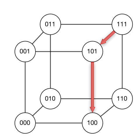
will begin with the hypercube routing algorithm [38, 39]. Consider a network topology (the hypercube) where each node is labeled by a bitstring of length and two nodes are connected by an edge if and only if the two corresponding labels differ in exactly one bit position.
In the network, there is initially one packet at each node, and each packet has a unique destination. The algorithm implements a routing strategy based on bit fixing: if the current position has bitstring , and the target node has bitstring , we compare the bits in and from left to right, moving along the edge that corrects the first differing bit. Valiant’s algorithm uses randomization to guarantee that the total number of steps grows logarithmically in the number of packets. In the first phase, each packet select an intermediate destination uniformly at random, and use bit fixing to reach . In the second phase, each packet use bit fixing to go from to the destination . We will focus on the first phase since the reasoning for the second phase is nearly identical. We can model the strategy with the code in Figure 18, using some syntactic sugar for the loops.77 7 Recall that the number of node in a hypercube of dimension is so each node can be identified by a number in .
We assume that initially, the position of the packet is at node (see Map.init). Then, we initialize the random intermediate destinations . The remaining loop encodes the evaluation of the routing strategy iterated time. The variable usedBy is a map that logs if an edge is already used by a packet, it is empty at the beginning of each iteration. For each packet, we try to move it across one edge along the path to its intermediate destination. The function getEdge returns the next edge to follow, following the bit-fixing scheme. If the packet can progress (its edge is not used), then its current position is updated and the edge is marked as used.
We show that if the number of timesteps is , then all packets reach their intermediate destination in at most steps, except with a small probability of failure. That is, the number of timesteps grows linearly in , logarithmic in the number of packets. This is formalized in our system as:
Modeling Infinite Processes.
Our second example is the coupon collector process. The algorithm draws a uniformly random coupon (we have coupon) on each day, terminating when it has drawn at least one of each kind of coupon. The code of the algorithm is displayed in Fig. 13; the array cp records of the coupons seen so far, t holds the number of steps taken before seeing a new coupon, and tracks of the total number of steps. Our goal is to bound the average number of iterations. This is formalized in our logic as:
Limited Randomness.
Pairwise independence says that if we see the result of , we do not gain information about all other variables . However, if we see the result of two variables , we may gain information about . There are many constructions in the algorithms literature that grow a small number of independent bits into more pairwise independent bits. Figure 14 gives one procedure, where is exclusive-or, and bits(j) is the set of positions set to in the binary expansion of j. The proof uses the following fact, which we fully verify: for a uniformly distributed Boolean random variable , and a random variable of any type,
| (1) |
for any two Boolean functions . Then, note that where the big XOR operator ranges over the indices where the bit representation of has bit set. For any two distinct, there is a bit position in where and differ; call this position and suppose it is set in but not in . By rewriting,
Since are all independent, follows from Eq. 1 taking to be the distribution on tuples excluding . This verifies pairwise independence:
Adversarial Programs.
Pseudorandom functions (PRF) and pseudorandom permutations (PRP) are two idealized primitives that play a central role in the design of symmetric-key systems. Although the most natural assumption to make about a blockcipher is that it behaves as a pseudorandom permutation, most commonly the security of such a system is analyzed by replacing the blockcipher with a perfectly random function. The PRP/PRF Switching Lemma [19, 6] fills the gap: given a bound for the security of a blockcipher as a pseudorandom function, it gives a bound for its security as a pseudorandom permutation.
Lemma 4 (PRP/PRF switching lemma).
Let be an adversary with blackbox access to an oracle O implementing either a random permutation on or a random function from to . Then the probability that the adversary distinguishes between the two oracles in at most calls is bounded by
where is a map storing each adversary call and is its size.
Proving this lemma can be done using the Fundamental Lemma of Game-Playing, and bounding the probability of bad in the program from Fig. 15. We focus on the latter. Here we apply the [Adv] rule of Ellora with the invariant where is the size of the map , i.e. the number of adversary call. Intuitively, the invariant says that at each call to the oracle the probability that bad has been set before and that the number of adversary call is less than is bounded by a polynomial in .
The invariant is -closed and true before the adversary call, since at that point . Then we need to prove that the oracle preserves the invariant, which can be done easily using the precondition calculus ([PC] rule).
8 Implementation and Mechanization
We have built a prototype implementation of Ellora within EasyCrypt [5, 2], a theorem prover originally designed for verifying cryptographic protocols. EasyCrypt provides a convenient environment for constructing proofs in various Hoare logics, supporting interactive, tactic-based proofs for manipulating assertions and allowing users to invoke external tools, like SMT-solvers, to discharge proof obligations. EasyCrypt provides a mature set of libraries for both data structures (sets, maps, lists, arrays, etc.) and mathematical theorems (algebra, real analysis, etc.), which we extended with theorems from probability theory.
| Example | LC | FPLC |
|---|---|---|
| hypercube | 100 | 1140 |
| coupon | 27 | 184 |
| vertex-cover | 30 | 61 |
| pairwise-indep | 30 | 231 |
| private-sums | 22 | 80 |
| poly-id-test | 22 | 32 |
| random-walk | 16 | 42 |
| dice-sampling | 10 | 64 |
| matrix-prod-test | 20 | 75 |
We used the implementation for verifying many examples from the literature, including all the programs presented in § 7 as well as some additional examples (such as polynomial identity test, private running sums, properties about random walks, etc.). The verified proofs bear a strong resemblance to the existing, paper proofs. Independently of this work, Ellora has been used to formalize the main theorem about a randomized gossip-based protocol for distributed systems [KempeDG03, Theorem 2.1]. Some libraries developed in the scope of Ellora have been incorporated into the main branch of EasyCrypt, including a general library on probabilistic independence.
A New Library for Probabilistic Independence.
In order to support assertions of the concrete program logic, we enhanced the standard libraries of EasyCrypt, notably the ones dealing with big operators and sub-distributions. Like all EasyCrypt libraries, they are written in a foundational style, i.e. they are defined instead of axiomatized. A large part of our libraries are proved formally from first principles. However, some results, such as concentration bounds, are currently declared as axioms.
Our formalization of probabilistic independence deserves special mention. We formalized two different (but logically equivalent) notions of independence. The first is in terms of products of probabilities, and is based on heterogenous lists. Since Ellora (like EasyCrypt) has no support for heterogeneous lists, we use a smart encoding based on second-order predicates. The second definition is more abstract, in terms of product and marginal distributions. While the first definition is easier to use when reasoning about randomized algorithms, the second definition is more suited for proving mathematical facts. We prove the two definitions equivalent, and formalize a collection of related theorems.
Mechanized Meta-Theory.
The proofs of soundness and relative completeness of the abstract logic, without adversary calls, and the syntactical termination arguments have been mechanized in the Coq proof assistant. The development is available in supplemental material.
9 Related Work
More on Assertion-Based Techniques.
The earliest assertion-based system is due to Ramshaw [34], who proposes a program logic where assertions can be formulas involving frequencies, essentially probabilities on sub-distributions. Ramshaw’s logic allows assertions to be combined with operators like , similar to our approach. [15] presents a Hoare-style logic with general assertions on the distribution, allowing expected values and probabilities. However, his while rule is based on a semantic condition on the guarded loop body, which is less desirable for verification because it requires reasoning about the semantics of programs. [7] give decidability results for a probabilistic Hoare logic without while loops. We are not aware of any existing system that supports assertions about general expected values; existing works also restrict to Boolean distributions. [35] formalize a Hoare logic for probabilistic programs but unlike our work, their assertions are interpreted on distributions rather than sub-distributions. For conditionals, their semantics rescales the distribution of states that enter each branch. However, their assertion language is limited and they impose strong restrictions on loops.
Other Approaches.
Researchers have proposed many other approaches to verify probabilistic program. For instance, verification of Markov transition systems goes back to at least [14, 37]; our condition for ensuring almost-sure termination in loops is directly inspired by their work. Automated methods include model checking (see e.g., [1, 22, 26]) and abstract interpretation (see e.g., [29, 11]). Techniques for reasoning about higher-order (functional) probabilistic languages are an active subject of research (see e.g., [bizjak2015step, 10.1007/978-3-642-54833-8_12, DalLago:2014:CEH:2535838.2535872]). For analyzing probabilistic loops, in particular, there are tools for reasoning about running time. There are also automated systems for synthesizing invariants [10, 3]. [8, 9] use a martingale method to compute the expected time of the coupon collector process for —fixing lets them focus on a program where the outer while loop is fully unrolled. Martingales are also used by [12] for analyzing probabilistic termination. Finally, there are approaches involving symbolic execution; [36] use a mix of static and dynamic analysis to check probabilistic programs from the approximate computing literature.
10 Conclusion and Perspectives
We introduced an expressive program logic for probabilistic programs, and showed that assertion-based systems are suited for practical verification of probabilistic programs. Owing to their richer assertions, program logics are a more suitable foundation for specialized reasoning principles than expectation-based systems. As evidence, our program logic can be smoothly extended with custom reasoning for probabilistic independence and union bounds. Future work includes proving better accuracy bounds for differentially private algorithms, and exploring further integration of Ellora into EasyCrypt.
Acknowledgments.
We thank the reviewers for their helpful comments. This work benefited from discussions with Dexter Kozen, Annabelle McIver, and Carroll Morgan. This work was partially supported by ERC Grant #679127, and NSF grants 1513694 and 1718220.
References
- [1] Baier, C.: Probabilistic model checking. In: Esparza, J., Grumberg, O., Sickert, S. (eds.) Dependable Software Systems Engineering, NATO Science for Peace and Security Series - D: Information and Communication Security, vol. 45, pp. 1–23. IOS Press (2016), http://dx.doi.org/10.3233/978-1-61499-627-9-1
- [2] Barthe, G., Dupressoir, F., Grégoire, B., Kunz, C., Schmidt, B., Strub, P.: Easycrypt: A tutorial. In: Aldini, A., Lopez, J., Martinelli, F. (eds.) Foundations of Security Analysis and Design VII - FOSAD 2012/2013 Tutorial Lectures. Lecture Notes in Computer Science, vol. 8604, pp. 146–166. Springer (2013)
- [3] Barthe, G., Espitau, T., Ferrer Fioriti, L.M., Hsu, J.: Synthesizing probabilistic invariants via Doob’s decomposition. In: International Conference on Computer Aided Verification (CAV), Toronto, Ontario (2016), https://arxiv.org/abs/1605.02765
- [4] Barthe, G., Gaboardi, M., Grégoire, B., Hsu, J., Strub, P.Y.: A program logic for union bounds. In: International Colloquium on Automata, Languages and Programming (ICALP), Rome, Italy (2016), http://arxiv.org/abs/1602.05681
- [5] Barthe, G., Grégoire, B., Heraud, S., Béguelin, S.Z.: Computer-aided security proofs for the working cryptographer. In: Rogaway, P. (ed.) Advances in Cryptology - CRYPTO 2011. Lecture Notes in Computer Science, vol. 6841, pp. 71–90. Springer (2011)
- [6] Bellare, M., Rogaway, P.: The security of triple encryption and a framework for code-based game-playing proofs. In: Vaudenay, S. (ed.) Advances in Cryptology - EUROCRYPT 2006, 25th Annual International Conference on the Theory and Applications of Cryptographic Techniques, St. Petersburg, Russia, May 28 - June 1, 2006, Proceedings. Lecture Notes in Computer Science, vol. 4004, pp. 409–426. Springer (2006), http://dx.doi.org/10.1007/11761679_25
- [7] Chadha, R., Cruz-Filipe, L., Mateus, P., Sernadas, A.: Reasoning about probabilistic sequential programs. Theoretical Computer Science 379(1-2), 142–165 (2007)
- [8] Chakarov, A., Sankaranarayanan, S.: Probabilistic program analysis with martingales. In: International Conference on Computer Aided Verification (CAV), Saint Petersburg, Russia. Lecture Notes in Computer Science, vol. 8044, pp. 511–526. Springer (2013)
- [9] Chakarov, A., Sankaranarayanan, S.: Expectation invariants as fixed points of probabilistic programs. In: Static Analysis Symposium (SAS). Lecture Notes in Computer Science, vol. 8723, pp. 85–100. Springer-Verlag (2014)
- [10] Chatterjee, K., Fu, H., Novotný, P., Hasheminezhad, R.: Algorithmic analysis of qualitative and quantitative termination problems for affine probabilistic programs. In: ACM SIGPLAN–SIGACT Symposium on Principles of Programming Languages (POPL), St Petersburg, Florida. pp. 327–342 (2016), http://doi.acm.org/10.1145/2837614.2837639
- [11] Cousot, P., Monerau, M.: Probabilistic abstract interpretation. In: Seidl, H. (ed.) 21st European Symposium on Programming, ESOP 2012. Lecture Notes in Computer Science, vol. 7211, pp. 169–193. Springer (2012)
- [12] Fioriti, L.M.F., Hermanns, H.: Probabilistic termination: Soundness, completeness, and compositionality. In: Rajamani, S.K., Walker, D. (eds.) Proceedings of the 42nd ACM Symposium on Principles of Programming Languages, POPL 2015. pp. 489–501. ACM (2015)
- [13] Gretz, F., Katoen, J.P., McIver, A.: Operational versus weakest pre-expectation semantics for the probabilistic guarded command language. Performance Evaluation 73, 110–132 (2014)
- [14] Hart, S., Sharir, M., Pnueli, A.: Termination of probabilistic concurrent programs. ACM Trans. Program. Lang. Syst. 5(3), 356–380 (1983)
- [15] den Hartog, J.: Probabilistic extensions of semantical models. Ph.D. thesis, Vrije Universiteit Amsterdam (2002)
- [16] Hurd, J.: Formal verification of probabilistic algorithms. Tech. Rep. UCAM-CL-TR-566, University of Cambridge, Computer Laboratory (2003)
- [17] Hurd, J.: Verification of the miller-rabin probabilistic primality test. J. Log. Algebr. Program. 56(1-2), 3–21 (2003), http://dx.doi.org/10.1016/S1567-8326(02)00065-6
- [18] Hurd, J., McIver, A., Morgan, C.: Probabilistic guarded commands mechanized in HOL. Theor. Comput. Sci. 346(1), 96–112 (2005)
- [19] Impagliazzo, R., Rudich, S.: Limits on the provable consequences of one-way permutations. In: Johnson, D.S. (ed.) Proceedings of the 21st Annual ACM Symposium on Theory of Computing, May 14-17, 1989, Seattle, Washigton, USA. pp. 44–61. ACM (1989), http://doi.acm.org/10.1145/73007.73012
- [20] Kaminski, B.L., Katoen, J.P., Matheja, C.: Inferring covariances for probabilistic programs. In: International Conference on Quantitative Evaluation of Systems. pp. 191–206. Springer (2016)
- [21] Kaminski, B., Katoen, J.P., Matheja, C., Olmedo, F.: Weakest Precondition Reasoning for Expected Run-Times of Probabilistic Programs. In: European Symposium on Programming (ESOP), Eindhoven, The Netherlands (Jan 2016)
- [22] Katoen, J.P.: The probabilistic model-checking landscape. In: Proceedings of LICS’16 (2016)
- [23] Kempe, D., Dobra, A., Gehrke, J.: Gossip-based computation of aggregate information. In: Foundations of Computer Science, 2003. Proceedings. 44th Annual IEEE Symposium on. pp. 482–491. IEEE (2003)
- [24] Kozen, D.: Semantics of probabilistic programs. In: 20th IEEE Symposium on Foundations of Computer Science, FOCS 1979. pp. 101–114. IEEE Computer Society (1979)
- [25] Kozen, D.: A probabilistic PDL. J. Comput. Syst. Sci. 30(2), 162–178 (1985)
- [26] Kwiatkowska, M., Norman, G., Parker, D.: PRISM 4.0: Verification of probabilistic real-time systems. In: Gopalakrishnan, G., Qadeer, S. (eds.) Proc. 23rd International Conference on Computer Aided Verification (CAV’11). LNCS, vol. 6806, pp. 585–591. Springer (2011)
- [27] McIver, A., Morgan, C.: Abstraction, Refinement, and Proof for Probabilistic Systems. Monographs in Computer Science, Springer (2005)
- [28] McIver, A., Morgan, C.: A new rule for almost-certain termination of probabilistic and demonic programs (2016), https://arxiv.org/abs/1612.01091, arXiv preprint arXiv:1612.01091
- [29] Monniaux, D.: Abstract interpretation of probabilistic semantics. In: Palsberg, J. (ed.) Static Analysis, 7th International Symposium, SAS 2000. Lecture Notes in Computer Science, vol. 1824, pp. 322–339. Springer (2000)
- [30] Morgan, C.: Proof rules for probabilistic loops. In: Proceedings of the BCS-FACS 7th Conference on Refinement. FAC-RW’96 (1996)
- [31] Morgan, C., McIver, A., Seidel, K.: Probabilistic predicate transformers. ACM Trans. Program. Lang. Syst. 18(3), 325–353 (1996)
- [32] Olmedo, F., Kaminski, B.L., Katoen, J.P., Matheja, C.: Reasoning about recursive probabilistic programs. In: Proceedings of the 31st Annual ACM/IEEE Symposium on Logic in Computer Science. pp. 672–681. ACM (2016)
- [33] Pearl, J., Paz, A.: Graphoids: Graph-based logic for reasoning about relevance relations. In: ECAI. pp. 357–363 (1986)
- [34] Ramshaw, L.H.: Formalizing the Analysis of Algorithms. Ph.D. thesis, Computer Science (1979)
- [35] Rand, R., Zdancewic, S.: VPHL: A Verified Partial-Correctness Logic for Probabilistic Programs. In: Mathematical Foundations of Program Semantics (MFPS XXXI) (2015)
- [36] Sampson, A., Panchekha, P., Mytkowicz, T., McKinley, K.S., Grossman, D., Ceze, L.: Expressing and verifying probabilistic assertions. In: O’Boyle, M.F.P., Pingali, K. (eds.) ACM Conference on Programming Language Design and Implementation, PLDI ’14. p. 14. ACM (2014)
- [37] Sharir, M., Pnueli, A., Hart, S.: Verification of probabilistic programs. SIAM J. Comput. 13(2), 292–314 (1984)
- [38] Valiant, L.G.: A scheme for fast parallel communication. SIAM journal on computing 11(2), 350–361 (1982)
- [39] Valiant, L.G., Brebner, G.J.: Universal schemes for parallel communication. In: Proceedings of the Thirteenth Annual ACM Symposium on Theory of Computing. pp. 263–277. STOC ’81, ACM, New York, NY, USA (1981), http://doi.acm.org/10.1145/800076.802479
Appendix 0.A Soundness of Ellora
Before presenting the proof of soundness, we will introduce two technical lemmas needed for the loop rules. Intuitively, - and -closed assertions are preserved in the limit of general and lossless loops, respectively.
Proposition 5.
- 1.
If is -closed and is s.t.
then .
- 2.
If is -closed and is s.t.
then , provided that is lossless.
Proof.
We only treat the first case; the second is similar. Let be a -closed assertion s.t. for any sub-distribution , if , then . We prove by induction on that for any sub-distribution such that , we have . By downward closedness of , we have . We conclude by -closenedness of . ∎
Lemma 6.
Let be an assertion and be a command. Then .
Proof.
Let . By definition of , this amounts to have , which exactly gives the expected result. ∎
Lemma 7.
Let be a sub-distribution and be a command. Then, .
Proof.
We have
Lemma 8.
Let be a sub-distribution s.t. where is a finite set, all the ’s are in and all the ’s are sub-distributions. Then, for any command ,
Proof.
Immediate consequence of the linearity of . ∎
Lemma 9.
Let be a lossless command and be a sub-distribution. Then .
Proof.
The proof is done by a direct induction of . ∎
Lemma 10.
The rules of Ellora are sound.
Proof.
We use the notation of the rules.
- •
[Skip] — immediate since .
- •
[Abort] — immediate by definition of and since
- •
[Assgn] & [Sample] — immediate consequence of Lemma 6.
- •
[Seq] — let . Then, by the first premise, . Hence, by the second premise, .
- •
[Conseq] — if , then by the first premise. Hence, by the second premise and by the third premise.
- •
[Split] — let . Then, there exists s.t. and for . By the two premises of the rule, we have for . Now, by Lemma 8, we have . By taking resp. and for the witnesses of , we obtain that .
- •
[Cond] — we first prove that
(2) Let . Then, for , we know that . It follows that
However, by the first premise, . Hence,
concluding the proof of Eq. 2. By a similar reasoning, we have:
(3) - •
[Call] — immediate consequence of [Seq] and [Assgn].
- •
[Frame] — let . Let . To show that , from the definition of , it is sufficient to show that and . The first one is a consequence of the losslessness of , the second one is a direct application of Lemma 9.
- •
[While] — from the first premise, by induction on and using [Seq], we know that for any , the following holds:
(4) Now, let . First, form the definition of , we know that
It remains to prove . In the case of certain termination, we know the existence of a s.t.
and we conclude by Eq. 4. For the cases of almost surely termination and almost termination, we conclude for Eq. 4 and Proposition 5 of the paper.
- •
[Adv] — the proof is done by induction on the body of the external procedure which is of the form where the ’s do not contain calls and the ’s are potential calls to the oracles. From the [Frame] rule, we know that the ’s preserve the invariant — noting that the losslessness of the adversary implies the losslessness of the ’s. Likewise, from the last premise of the [Adv] rule, we know that calls to the oracles also preserve the invariant. Hence, by multiple application of the [Seq] rule, we obtain that the adversary body maintains . ∎
Appendix 0.B Semantics of Assertions
The semantics of assertions is given Fig. 16.
Appendix 0.C Precondition Calculus
Figure 17 contains the full definition of the precondition calculus.
Appendix 0.D Soundness of the Syntactic Rules
0.D.1 Certain Termination
Proposition 11 (Soundness of rule [While-]).
Let be a sub-distributions such that is valid. Then,
Proof.
Given satisfying , we first claim that there exists a decreasing function such that holds at each iteration of the loop. Indeed, we remark that the statement holds at first iteration by the precondition hypothesis. Let:
Then unrolling the loop and using the semantical [Seq] rule ensure by induction the claimed domination. The termination of the loop arises then naturally from the exit condition . ∎
0.D.2 Almost-Sure Termination
The main challenge for proving the soundness of the is proving termination; from there, we can conclude by rule [While-]. Our arguments use basic notations and theorems from the theory of Markov processes.
Proposition 12 (Soundness of rule [While-]).
Let be a -closed assertion. For any sub-distributions , such that is valid. Then
Proof.
As indicated, by soundness of the semantic while rule for almost-sure termination, and the premises, it suffices to prove almost-sure termination. The sketch of the proof is the following:
- 1.
We follow the behavior of the variant by seeing it as a random variable on the space of state.
- 2.
We first introduce a Markov chain that reaches a particular state (the state zero) with probability .
- 3.
We then stochasticaly dominates the variant by the latter chain.
- 4.
In particular, this shows that the probability of the variant to eventually reach is , ensuring almost-sure termination.
Step one: Variant as a Random variable.
We consider the integer-valued variant as a random variable
over the space of states. Let the family represents the value taken by
after the -th iteration of the loop.
Then we have, using the semantical rule and the
- •
The sequence is uniformly bounded by .
- •
The probability of decreasing is bounded below by :
Step two: Modelization with a Markov chain.
First, we can assume that since if , the loop terminates
immediately.
Consider the following finite Markov chain , over the state
space , following the transitions:
This chain models the following behavior: with probability the value decrease by one, while with probability it jumps to . Since zero is the only connected component of the underlying graph, the probability of terminating in the state zero is by a standard result on Markov chains.
Step three: Stochastic domination.
By construction, there exists a natural coupling between and
, since the probability of the event decrease
is greater than the probability of the event decrease.
Since we impose that
(initial position), a simple induction over ensure that we have, for this coupling:
, so
as desired.
∎
Appendix 0.E Further Examples
0.E.1 Randomization for Approximation: Vertex Cover
We begin with a classical application of randomization: approximation algorithms for computationally hard problems. For problems that take long time to solve in the worst case, we can sometimes devise efficient algorithms that find a solution that is “nearly” as good as the true solution.
Our first example illustrates a famous approximation algorithm for the vertex cover problem. The input is a graph described by vertices and edges . The goal is to output a vertex cover: a subset such that each edge has at least one endpoint in , and such that is as small as possible.
It is known that this problem is NP-complete, but there is simple randomized algorithm that returns a vertex cover that is at on average at most twice the size of the optimal vertex cover. The algorithm proceeds by maintaining a current cover (initially empty) and considering each edge in order. If neither endpoint is in current cover, the algorithm adds one of the two endpoints uniformly at random. The Ellora program is:
Here, we represent edges as a finite set of pairs of nodes. We loop through the edges, adding one point of each uncovered edge to the cover C uniformly at random. The operator returns if b is true, and if not.
To prove the approximation guarantee, we first assume that we have a set of nodes . We only assume that is a valid vertex cover; i.e., each edge has at least one endpoint in . Then, we use the following loop invariant:
| (5) |
Given the loop invariant, we can prove the conclusion by letting be the cover of minimal size, and reasoning about intersections and differences of sets.
Clearly the invariant is initially true. To see why the invariant is preserved, let e be the current edge, with both endpoints out of C. Since is a vertex cover, it has at least one endpoint of e. Since our algorithm includes an endpoint of e uniformly at random, the probability we choose a vertex not in is at most , so the expectation on the left in Eq. 5 increases by at most . If e is not covered in C but is covered by , there is at least a probability that we increase the intersection , so the right side in Eq. 5 increases by at least . Thus, the invariant is preserved, and we can prove
and by reasoning on intersection and difference of sets,
0.E.2 Random Walks: Termination and Reachability
A canonical example of a random process is a random walk. There are many variations, but the basic scenario describes a numeric position changing over time, where the position depends on the position at the previous timestep, influenced by random noise drawn from some distribution.
To demonstrate how to verify interesting facts about random processes, we will model a one-dimensional random walk on the natural numbers. We start at position , and repeatedly update our position according to the following rules. From , we always make a step to . From non-zero positions, we flip a fair coin that is biased to come up heads with probability . If heads, we increase our position by ; if tails, we decrease by .
We will prove two facts about this random walk. First, for any natural number , the probability of eventually reaching is . Second, when we reach , we must first pass through all intermediate points . In Ellora, we can express the random walk with the following code.
In order to verify this example, we will use the probabilistic while rule [While-ASTerm]. First we establish almost-sure termination by finding an appropriate termination measure: the distance between our current position, and T. Indeed, this measure is bounded by T, and has a non-negative (at least ) probability of decreasing each iteration. Therefore, the loop terminates almost-surely, and thus our random walk eventually reaches any point T with probability .
To prove our second assertion—that we visit every point from to T—we use the following loop invariant for the while command:
In other words, if we have reached position pos, then we must have already reached every position in . Since this invariant is -closed, we may apply rule [While-ASTerm] and the invariant holds at the end of the loop. With the assertion at termination, we have enough to prove that each position is visited:
The losslessness post-condition indicates that the walk terminates almost-surely.
0.E.3 Amplification: Polynomial Identity Testing
A second use of randomness is in running independent trials of the same algorithm. This technique, known as probability amplification, runs a randomized algorithm several times in order to reduce the error probability. Roughly speaking, a single trial may have high error with some probability, but by repeating the trial it is unlikely that all of the trials yield poor results. By combining the results appropriately—e.g., with a majority vote for algorithms with binary outputs, or by selecting the best answer when we can check the quality of the solution—we can produce an output that is more accurate than a single run of the original algorithm.
An example in this vein is probabilistic polynomial identity testing. Given two multivariate polynomials and over the finite field of elements, we want to check whether , or equivalently, whether the polynomial is zero or not. We will take uniformly random samples from and check whether . We repeat the trial times, rejecting if we see a sample where the difference is non-zero. In our system, this corresponds to the following program:
The proof uses an instance of the Schwartz-Zippel lemma due to Øystein Ore for finite fields, which upper bounds the probability of randomly picking a root of a polynomial over a finite field.
Lemma 13.
Let a non-zero polynomial function over . If we sample the variables uniformly at random from , then
We encode this lemma as an axiom in our system:
With this fact, we can prove the following loop invariant:
finally proving that
We have also verified Freivald’s algorithm, an amplification-based algorithm for checking matrix multiplication.
0.E.4 Concentration Bounds: Private Running Sums
Now, we turn to examples involving independence of random variables. Our first example is drawn from the differential privacy literature. Given a list of integers, we add noise from a two-sided geometric distribution to each entry in order to protect privacy, and we calculate the partial sums of the noisy values: , and so on. We wish to measure how far the noisy sums deviate from the true sums.
In Ellora, we can express this algorithm as follows:
The parameter to the noise distribution twogeom is a numeric parameter controlling the strength of the privacy guarantee, by changing the magnitude of the noise.
Our loop invariant tracks three pieces of information: (i) noise[i] is distributed according to ; (ii) the array noise remains independent; and (iii) out[i] stores the noisy running sum:
To bound the error introduced by the noise, we need to bound . Since we know that the elements in noise are all independent, we can apply a concentration bound to bound the probability of a large error in the -th running sum, concluding:
for a particular function derived from the Berry-Esseen theorem.
0.E.5 Hypercube Routing in More Details
We will begin with the hypercube routing algorithm [38, 39]. To set the stage, consider a network where each node is labeled by a bitstring of length , and two nodes are connected by an edge if and only if the two corresponding labels differ in exactly one bit position. This network topology is known as a hypercube, a -dimensional version of the standard cube; a simple example with is in Fig. 18.
In the network, there is initially one packet at each node, and each packet has a unique destination. Our goal is to design a routing strategy that will move the packets from node to node, following the edges, until all packets reach their destination. Furthermore, the routing should be oblivious: to avoid coordination overhead, each packet must select a path without considering the behavior of the other packets.
To model the flow of packets, each packet’s current position is a node in the graph. Time proceeds in a series of steps, and at each step at most one packet can traverse any single edge. If several packets try to use the same edge simultaneously, one packet will be selected to move (for any selection strategy that selects some packet). The other packets wait at their current position; these packets are delayed and make no progress this step.
The routing strategy is based on bit fixing: if the current position has bitstring , and the target node has bitstring , we compare the bits in and from left to right, moving along the edge that corrects the first differing bit. For instance, if we are at and we wish to reach , we will move along the edge corresponding to the second position: from to , and then along the edge corresponding to the third position: from to . See Fig. 18 for a picture.
While this strategy is simple and oblivious, there are permutations that require a total number of steps growing linearly in the number of packets to route all packets. Valiant proposes a simple modification, so that the total number of steps grows logarithmically in the number of packets. In the first phase, each packet will first select an intermediate destination uniformly at random from all nodes, and use bit fixing to reach . In the second phase, each packet will use bit fixing to go from to the destination . We will focus on the first phase, since the reasoning for the second phase is nearly identical. We can model the strategy with the following code, using some syntactic sugar for the loops; recall that the number of node in a hypercube of dimension is so each node can be identified by a number in .
We assume that initially the position of the packet is at node (see Map.init). Then, we initialize the random intermediate destinations . The remaining loop encodes the evaluation of the routing strategy iterated time. The variable usedBy is a map that logs if an edge is already used by a packet, it is empty at the beginning of each iteration. For each packet, we try to move it across one edge along the path to its intermediate destination. The function getEdge returns the next edge to follow, following the bit-fixing scheme. If the packet can progress (its edge is not used), then its current position is updated and the edge is marked as used.
Our goal is to show that if the number of timesteps is , then all packets reach their intermediate destination in at most steps, except with a small probability of failure. That is, the number of timesteps grows linearly in , logarithmic in the number of packets. At a high level, the analysis involves three steps.
The first step is to consider a single packet traveling from to , and to calculate the average number of other packets that share at least one edge with ’s path . Let be if the paths of packets and share at least one edge and otherwise. Then, the load on ’s path is the sum of over all the other packets . By using the fact that each intermediate destination in is uniformly distributed, and by analyzing the number of packets beside ’s that use each edge on ’s path, we can upper bound the expected value of by . In the second step, we move from a bound on the expectation of to a high-probability bound: we want to show that holds except with a small probability of failure. The key tool is the Chernoff bound, which gives high probability bounds of sums of independent samples. The libraries in Ellora include a mechanized proof of a generalized Chernoff bound, with the following statement (leaving off some of the parameters):
Returning to the proof, we bounded the expectation of in the previous step. To apply the Chernoff bound, we need to show that for any packet , the expressions are independent for all . This is not exactly true, since and both depend on the (random) destination of packet . However, it suffices to show that these variables are independent if we fix the value of ; then we can apply the Chernoff bound to upper bound with high probability.
Finally, we can bound the total delay of any packet. This portion of the proof rests on an intricate loop invariant assigning an imaginary coin for each delay step to some packet that crosses . By showing that each packet holds at most one coin, we can conclude that the ’s delay is at most the number of crossing packets. With our high probability bound from the previous step, we can show that timesteps is sufficient to route all packets to , except with some small probability:
0.E.6 Coupon Collector in More Details
Our second example is the coupon collector process. The algorithm draws a uniformly random coupon (we have coupon) on each day, terminating when it has drawn at least one of each kind of coupon. The code of the algorithm is as follows.
The array cp keeps track of the coupons seen so far; initially . We divide the loop into a sequence of phases (the outer loop) where in each phase we repeatedly sample coupons and wait until we see a new coupon (the inner loop). We keep track of the number of steps we spend in each phase in , and the total number of steps in .
Our goal is to bound the average number of iterations. The code involves two nested loops, so we have two loop invariants. The inner loop has a probabilistic guard: at every iteration, there is a finite probability that the loop terminates (i.e., if we draw a new coupon), but there is no finite bound on the number of iterations we need to run. Since our desired loop invariant is not downwards closed, we must apply the rule for almost sure termination. We use a variant that is if we have not seen a new coupon, and if we have seen a new coupon. Note that each iteration, we have a strictly positive probability of seeing a new coupon and decreasing the variant. Furthermore, the variant is bounded by , and the loop exits when the variant reaches . So, the side-condition holds. For the inner loop, we prove that forall the invariant is preserved:
Note that this is a -closed formula; there is an existential in the second disjunction, but it has finite domain (for fixed ).
For intuition, for every natural number there are two cases: Either we have already unrolled more than iterations, or not. The first disjunction corresponds to the first case, since loops where the guard is true all have , and the probability of stopping at iterations is —we see old coupons, and then a new one. Otherwise, we have the second disjunction. The integer represents the current number of unfoldings of the loop. If the loop is continuing then . If the loop is terminated, it terminated before the current iteration: . Furthermore, the probability of continuing at iteration is . At the end of the loop we have . So, by the first conjunct and some manipulations,
holds when the inner loop exits, precisely describing the distribution of iterations ct as by definition.
The outer loop is easier to handle, since the loop has a fixed bound on the number of iterations so we can use the rule for certain termination. For the loop invariant, we take:
The first conjunct states that the previous waiting times follow a geometric distribution with parameter ; this assertion follows from the previous reasoning on the inner loop. The second conjunct asserts that holds the total waiting time so far. The final two conjuncts state that there are at most flags set in cp. Thus,
at the end of the outer loop. By applying linearity of expectations and a fact about the expectation of the geometric distribution, we can bound the expected running time: